Development of a high contrast Nd:glass laser using chirped pulse amplification

(1)

Development of a High Contrast

Nd:Glass Laser

Using Chirped Pulse Amplification

by

Yanjie Wang

February 1993

A thesis submitted for the degree of

Doctor of Philosophy

(2)

This thesis is entirely my own work,

except where explicitly indicated.

Yanjie Wang

Laser Physics Centre

Research School of Physical Sciences and Engineering

The Australian National University

(3)

Acknowledgements

I wish to thank my supervisor, Prof. Barry Luther-Davies, for his direct guidance

throughout the whole of this PhD program. Without his kind support and unwavering

confidence in me, I would have never started this project. I have benefited from his

wide-ranging experience, in particular, his experimental expertise in laser physics. I

greatly appreciate his many hours spent proof reading this thesis, and his comments and

suggestions on the thesis have been very valuable.

With great affection and respect, I would like to remember my late supervisor, Dr.

Ranko Dragila, who introduced me to the field of laser-plasma interactions, although this

part of my work is not included in this thesis. I feel deeply in my heart the loss of such

a wonderful person, who was warm-hearted and good-humoured, but I am fortunate to

have imitated his interest in fishing.

I am very grateful to the technical staff in our Centre, particularly Wally Hopkinson,

Paul Morrison, Michael Pennington, Ian McRae and Craig McLeod, for their technical

support Without their expertise, the progress in the laboratory experiments would have

been restricted

I wish to thank the secretary of our Centre, Mrs. Di Hodges, who has given me

much help in numerous ways. Her wonderful and charming personality has made this

Centre a very pleasant working place. I am grateful to the academic staff and the fellow

students o f our Centre for their friendliness and help. I also acknowledge the assistance

from the staff of the school computer unit.

My special thanks go to my wife, Chunshi Cui, who has been supportive and

understanding throughout the whole of my PhD work.

I would like to thank DITAC who financially sponsored my visit to the Laboratory

for Laser Energetics, University of Rochester. I wish to thank the Rochester group for

(4)

Chapter 4), and gratefully acknowledge the cooperation with Prof. D. D. Meyerhofer,

Dr. R. S. Craxton and Dr. Y. H. Chuang of that group.

Finally, I want to thank the Australian National University which provided me with

a scholarship to carry out this research and particularly R.S.Phys.S.E. which extended

(5)

(6)

Abstract

A chirped-pulse amplification (CPA) Nd:glass laser using a fiber-grating compression system has been studied through modelling and experiments. Special effort has been made to improve the intensity contrast ratio o f the pulses generated from this laser.

In this thesis, we report on the development o f a fiber-grating CPA Nd.glass laser which can produce 1.2 ps pulses with an energy o f > 3 J at 1.053 /im. The contrast ratio o f the pulses generated from such lasers is normally very low (< 100). To enhance the contrast, the spectral shaping method was numerically and experimentally studied. By applying this technique, the intensity contrast ratio o f the pulses from the laser was improved to > 103.

To further improve this contrast ratio, second harmonic generation was investigated through computer simulation. The modelling results have shown that a contrast en hancement close to R 2 (where R is the contrast ratio o f the fundamental pulse) can be achieved. Hence, frequency doubling can improve the contrast o f the pulses from the laser system from > 103 to > 106. More importantly, it has been found that for frequency doubling o f a ~ 1 ps laser pulse at - 1 /im in KDP (II), the group velocity mismatch between the interacting pulses can be used to advantage by pre-delaying the extraordinary (e) relative to the ordinary (o) pulses appropriately at the entrance to the crystal. In the optimal conditons, the power conversion efficiency from the fundamental to the second harmonic can be as high as 300%, and simultaneous “compression” of the output pulse duration can reach a factor o f four.

(7)

experimental results were in excellent agreement with the predictions of the computer

models.

To further increase the contrast, a new method using an optical parametric amplifica

tion based pre-pulse eliminator (OPAPE) has been proposed and its performance studied

through numerical modelling. It has been found that the contrast can be significantly

enhanced from R to ~ R3. For our CPA Nd laser system, we predict an increase in the contrast ratio from > 103 (after spectral shaping) to > 108. Moreover, frequency

doubling such a pulse can give a SH beam with a contrast higher than 1016. This

value should be sufficient enough to support any conceivable experiments involving

(8)

C hapter 1

In troduction

Recently, there have been significant advances in the development of high power

ultra-short (ps and sub-ps) pulsed lasers. High power ultra-short optical pulses have

been generated by using excimer lasers [21, 51, 108]; dye lasers [66]; CO2 lasers [12];

and via chirped pulse amplification (CPA) using Ndiglass [97] or Ti:sapphire/Nd:glass

lasers [85]. Powers from ~ 1 to > 50 TW [85] are now available from those sys

tems with sufficiently good beam quality to produce focussed pulse intensities from

1013 to IO20 W /cm 2. Such high intensity ultra-short pulse lasers have many ap

plications, and permit, for example, the study of solid-state density laser-matter

interactions [22, 38, 47, 62, 67]; high-order harmonic generation [48, 49, 59, 61];

multiphoton ionization [9, 46, 52]; above threshold ionization [13, 27]; and

ultra-short pulse X-ray lasers [31]. Intensities above I A2 > 1018 W /im2/cm 2 can be used

to accelerate plasma electrons to relativistic velocities [53] and provide the opportu

nities for studying light-light scattering [16]; induced vacuum polarization [53]; and

pair-production [8, 89]; which are basic predictions of quantum electrodynamics that

have never been observed.

Many applications require a high intensity contrast (i.e. the ratio of the maxi

mum intensity in the main pulse to the level of pre-pulse emission). For example, in

high intensity ultra-short pulse laser-matter interaction experiments, if the pre-pulse

has an intensity above the plasma production threshold, it can generate a low den

(12)

alter the physics of the ultra-short pulse interaction with matter. The aim of this thesis is to develop a very high contrast CPA Ndrglass laser.

1.1 T h e C o n cep t o f C h irp ed P u ls e A m p lifica tio n

In what follows we will focus upon ultra-short pulse amplification in solid-state amplifying media.

To amplify ultra-short pulses, three major requirements have to be satisfied by the amplifying medium [55]. Firstly, the gain linewidth of the amplifier has to be larger than the frequency bandwidth of the ultra-short pulse. Secondly, for efficient energy extraction, the fluence of the pulse has to be in the range of the amplifier saturation fluence Fa = hv/cr, where h is Planck’s constant, v is the laser frequency and or is the stimulated emission cross section. Finally, the pulse intensity must be below the critical value above which the intensity dependent index of refraction may cause serious wave front distortion.

In the available large bandwidth media, broad bandwidth solid-state materials, such as, Nd:glass; Ti:sapphire; Cr:LiSAF etc, are the most attractive amplifying media due to their high saturation fluence. For solid-state amplifying media, the saturation fluence is of the order of 5 J/cm 2 which is more than a thousand times larger than that of dye and excimer amplifiers. Thus it is possible to amplify a pulse energy to > 1 J using a relatively small scale solid-state amplifier.

(13)

in a solid-state amplifier because refractive index non-linearities become serious at intensities of the order of 10 GW/cm2, and hence the laser can only be operated at a maximum intensity around a few GW /cm2. When amplifying a 1 ps pulse to this maximum intensity, the fluence of the pulse is only a few m J/cm 2, i.e. far below the saturation fluence. However, this limitation can be overcome by using the chirped pulse amplification (CPA) technique [97].

To amplify a ps or sub-ps pulses using the CPA technique, the first step is to stretch the pulses using a grating-pair pulse stretcher [57] to generate a linearly frequency chirped pulse much longer than the original (durations range from a few hundred ps to about 1 ns). The next step is to amplify the stretched, chirped pulses to near the saturation energy of the laser amplifier whilst keeping its peak intensity below the critical value for non-linear effects. The final step involves recompression of the amplified, chirped pulse to the original pulse duration using a grating-pair pulse compressor [103]. By applying the CPA technique in a Ndiglass amplifier, a ~ 1 ps pulse with an energy of the order of 30 J has been achieved [85, 113].

1.2 P r o b le m s w ith C P A L asers

(14)

microsec-onds which allowed it to be pumped easily by flashlamps on a large scale. For this reason, most of high energy (> 1 J) solid-state CPA lasers operate at Ndiglass lasing wavelengths of ~ 1 fim.

Unfortunately, most Nd laser oscillators capable of generating pulse durations < 1 ps at ~ 1 /im, such as additive-pulse mode-locked (APM) lasers [29, 43, 56, 92], were still in the stage of laboratory study and had generally poor stability when this work commenced. Additionally, sub-100 fs pulse oscillators based on TiiSapphire are also a very recent innovation although they are now capable of providing seed pulses matching the Nd:glass wavelength. However, these innovations have come rather late for the current generation of CPA Ndiglass laser systems which are based on the fiber-grating pulse compression scheme to generate ultra-short pulses starting with a relatively long pulse from a conventional lamp-pumped mode-locked NdiYAG or Nd:YLF laser oscillator [10, 24, 55, 76, 77, 87, 97]. For applications of these lasers, such as the study of ultra-short laser pulse interactions with matter, a very high intensity contrast ratio is essential. Due to the poor intensity contrast ratio (< 100) associated with a normal fiber-grating pulse compression scheme, the elimination of the pre-pulse emission is a major problem when developing such systems.

(15)

et al. [73] and studied by many other reseachers [30, 84, 111]. Recently, Beaudoin

et al. [4] applied this technique to a CPA laser, and obtained a contrast ratio of

> 106. Using a fast Pockels cell to select the central portion of the pulse (where the frequency is linear chirped) before amplification and compression, Yamakawa et al

[113] achieved a contrast ratio of > 107, which is the highest contrast ratio that has yet been reported.

At present, focussed intensities of lO20 W /cm 2 are available, and in the next few years, the rapid development of CPA lasers should be possible to increase this intensity to the range of 1021 to 1023 W /cm 2. However, the highest intensity contrast is about 107 at present, which is far below that required in many applications. Hence, enhancing the intensity contrast is still an major issue in the development of high intensity ultra-short pulse CPA lasers. Note that even if the problems associated with fiber-grating CPA lasers can be overcome, amplified spontaneous emission (ASE) from the amplifiers also can generate low intensity, long pre-pulses and can limit the maximum contrast ratio that can be achieved in a CPA laser [53], and ultimately this source must be eliminated.

In this work, we have developed a high contrast CPA Nd:glass laser system (based on a fiber-grating pulse compression scheme) at the Australian National University. To improve the intensity contrast, the techniques of spectral shaping, frequency doubling and optical parametric amplification have been studied in detail. Using the combination of these techniques, an intensity contrast ratio of > 108 for pulses at 1.053 fim and of > 1016 at 0.527 fim can be obtained from the CPA laser.

1.3 Thesis Outline

Chapter 2 is devoted to numerical modelling of the fiber-grating pulse compressor for determining the sources which lead to the pre-pulse emission. In addition, numerical modelling of contrast improvement using spectral shaping is also presented.

(16)

the experimental results on contrast improvement based on the spectral shaping technique.

Since the spectral shaping method has its limitations in improving the intensity contrast, several other techniques have been explored in this study. A numerical study of highly efficient second harmonic conversion of ~ 1 ps Nd laser pulses using group velocity mismatched frequency doubling in KDP is presented in Chapter 4. The intensity contrast improvement using frequency doubling is also numerically studied in this chapter.

In Chapter 5, the experiments on second harmonic conversion using group ve locity mismatched frequency doubling are described and the results demonstrating very high conversion efficiencies are presented. These experimental results are found in excellent agreement with what was predicted in Chapter 4.

(17)

C hapter 2

A N um erical S tu d y o f a

F iber-grating P u lse C om pressor

Optical pulse compression using a fiber-grating pulse compressor has become a stan dard technique for reducing the pulse duration outside a laser cavity [17, 26, 37, 41, 73, 75, 98]. The principle of this technique can be described as follows. When a bandwidth-limited optical pulse is launched into a single mode optical fiber, self phase modulation (SPM) generates new frequencies in the power spectrum at dif ferent times during the pulse. At the same time, group velocity dispersion (GVD) increases the pulse duration. At the fiber output, an approximately linearly fre quency chirped pulse with a rectangular envelope is formed by the combined effects of SPM and GVD. Subsequently, the pulse can be compressed to a new bandwidth limit by a parallel grating pair, which introduces a frequency dependent time delay which recombines the frequency components of the pulse in the time domain.

(18)

parallel grating pair is employed to compress the pulse to a much shorter duration

than available at the input to the fiber. Recently this kind of laser system has been

proven able to produce a focussed intensity over lO20 W /cm 2 [85]. However, the

useful intensity level is still limited by the pre-pulse emission associated with the

compressed pulse.

The aim of this chapter is to use numerical modelling of a fiber-grating pulse

compressor to determine the sources which lead to the pre-pulse emission. The

chapter is organized as follows. The modelling of optical chirped pulse generation

and compression are presented in Section 1 and Section 2 respectively. Section 3

is devoted to a discussion of the sources which cause the pre-pulse emission on the

compressed pulse. Section 4 is devoted to the numerical modelling of the contrast

improvement using spectral shaping. A summary is given in Section 5.

2.1 M o d e llin g O p tica l C h irp ed P u ls e G en era tio n

in a S in gle M o d e O p tica l F ib er

2.1.1 Nonlinear Schrödinger Equation

In a single mode optical fiber, the refractive index can be expressed by [32]:

where no is the linear refractive index; the imaginary part, x> represents loss in the

fiber; and «2 describes the intensity dependence of the nonlinear refractive index. Consider an optical pulse having an electrical field

which propagates in + z direction. Here £ is the envelope of the electric field; u;0

and k0 are the centre carrier frequency and wave vector respectively. If we assume

that the electric field envelope £ varies slowly compared with the carrier and that (2.1)

E ( z , t ' ) = £ ( z , t ' ) exp[—i(yjQt' — k0z)\ (2.2)

(19)

mode optical fiber can be described by the nonlinear Schrödinger equation (in MKS units) [32, 65, 69]:

. ( d e

,

d s \

l (d^ + l£ + k'dF)

J W ~ 2n0k°l£l £

k2d2E 1 n2j (2.3)

where k0 = u?0no/c, c is speed of light in the vacuum; kx = dk/du 1^ is the inverse of the group velocity; k2 = d2k/duj21^ represents GVD, and 7 = xiôô/ô is the exponential decay factor.

Equation 2.3 can be reduced to a dimensionless equation [100]

O u . 7T

d( = ~ l 4

by the transformation

s = t

h ’

t = t' — k xz

4 =

z 1r t \

Z o ~ 2 |fc2 |

e _<• ₍ _{^ 0}

U —

£1 ’ \ l n 2 ZQ

r = I Z o

(2.4)

(2.5)

(2.6)

(2.7)

(2.8)

where t\ is an arbitrary constant which is usually taken as the pulse duration; t is the retarded time variable and corresponds to calculating the pulse shape in the frame of reference moving at the group velocity fcf1, and the centre of the pulse for any distance z along the fiber is at t = 0; zq and £\ are the normalized length and electric field respectively; and finally « = k2/\k2\ is sign of the group velocity dispersion. In the case of positive (normal) GVD, ac = 1, whilst k = — 1 corresponds

to negative (anomalous) GVD.

2.1.2 A lgorithm

(20)

u(^+A^,s) u(^+A^,s)

S P M +G V D +L oss

Figure 2.1: An optical pulse propagating through a thin segment of a fiber, £— £ -f A£, is equivalent to pulse propagation through three fibers that have the same thickness with only SPM, GVD and loss, present in each one respectively.

they still can be considered separately for a very thin segment of fiber. Consider an optical pulse propagating through a fiber from £ to £ + A£. Theoretically, if A£ is small enough, the combined effects of SPM, GVD and loss are equivalent to the sum of the individual effects (See Figure 2.1). Mathematically, we can split the Equation 2.4 into three equations

d u .7T , .9

—— = l — \ U \ U

d ( 2

(SPM only) (2.9)

d u . 7rd 2u

d £ ~ lK 4 d s 2

(GVD only) (2.10)

d u

W =

- r u

(loss only) (2.11)

Solving the above equations in the fiber from £ to f 4- A£, we obtain

u(f + A £,s) = ti({,s) exp(z^|u(£,s)|2A£) (SPM only) (2.12)

y + o o r y + o o

ti(f + A £,s) = / / u(£, 5) exp(—iAuAs) ds

J—00 \.J—00

x exp(z/c^Ao/2A£) exp(z‘Au/s) d(Au//27r) (GVD only)(2.13)

u(f + A £,s) = u(£,s) exp(—TA£) (loss only) (2.14)

After considering the combined effects of SPM, GVD and linear loss, u(f + A f,s) can be written in the following form, by using Equations 2.12, 2.13 and 2.14

u({ + A f , s ) = exp(—TAf) / / u({,s) e x p (i-|u ({ ,s)|2A{) exp(-iA u/s) ds

(21)

x exp(i/c jAü/ 2A£) exp(zAü/s) d(Au//27r) (2.15)

where Aw' = Au;T0 = (u — co0)T0. The formula 2.15 gives the relation u(£ +

A £ ,s) in the terms of u (£,s). To obtain u(( + A £ ,s), the Fast Fourier Transform

(FFT) technique [81] can be used to calculate the (inverse) Fourier transform in

Equation 2.15 when u(£,s) is known. Hence, when the initial condition u(£ = 0 ,s)

is given, we can calculate the pulse envelope at any distance along the fiber by

repeatedly using Equation 2.15. Convergence of the calculations can be achieved by

reducing A£ until the output pulse envelope no longer changes.

In Equation 2.15, all the dimensionless parameters can be easily calculated from

Equations 2.5, 2.6, 2.7 and 2.8. Assuming an input pulse envelope:

u ( 0 , i - ) = A sech(1.76^ -) (2.16)

JO Jo

where T0 is the pulse duration (FWHM of the intensity). According to Equation 2.7

the amplitude A can be expressed as:

A-i

(2.17)

Where P0 is the peak power of the input pulse and Pi is the normalized power which

can be expressed as follows in the MKS units:

= "°Aü '4.e/J x 107 ( W ) 167rcn2^o

where e0 and are the permittivity and permeability of free space respectively.

A ej j is the effective core area which for typical fiber parameters is fairly close to the

actual core area [101]. Taking t x = T0 from Equation 2.6, the normalized length z0

can be rewritten as

* 2cT02

A§|Z)|

by means of the relation D = (27rc/Aq)At2; where D is the GVD which is normally

given in units of ps/nm /km (MKS units must be used in Equation 2.19). Finally,

the loss in an optical fiber is normally given in units of dB/km . In this case:

r = 0.11151 ß z 0 (2.20)

(22)

2.1.3 Frequency Chirped P u lse Form ation

To demonstrate linearly chirped pulse formation in a single mode optical fiber, Equation 2.15 has been solved numerically under the conditions: A = 100, T = 0 (lossless), k = 1 (positive GVD) for the input pulse envelope given by Equation 2.16.

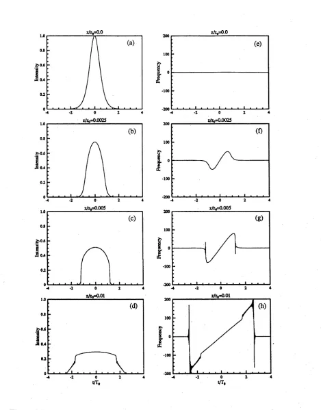
The results are shown in Figure 2.2. The left column shows the intensity as a function of time for various fiber lengths, and the right column shows the instan taneous frequency as a function of time corresponding to the pulse envelope of the left column. If we write u ( ( , t / T 0) = \u(£,t/T0)\ exp[z^>(</T0)], the instantaneous frequency is:

(23)

Figure 2.2: The intensity as a function of time (left column) and instantaneous frequency

[image:23.549.63.532.52.651.2]

(24)

2.2 G ratin g-p air P u ls e C o m p resso r

When a positively chirped pulse (whose frequency increases with time) passes through a negative linearly dispersive delay line, because the high frequencies trailing edge of the pulse travels faster than the low frequency leading edge in the delay line, we can adjust the delay line so that trailing and leading edges of the pulse emerge from the delay line at same time. Hence the output pulse can be much shorter than the input pulse, or we say that the pulse is compressed. In the picosecond pulse region, a parallel grating pair can act as a positively chirped pulse compressor.

2.2.1 Frequency D ependent P h ase Shift

When an optical pulse passes through a pair of parallel gratings, the different fre quencies of the pulse follow different paths and experience different group delays. It has been shown that [103] the group delay r is equal to d $ /d u , where $ is the frequency dependent phase shift which will be derived in this section. It has also been proven that [7] the group delay is exactly equal to the path delay, that is

d<t> l(u)

T “ f a ~ ~

where / is the optical length through the grating pair as a function of frequency, c is the speed of light in the vacuum.

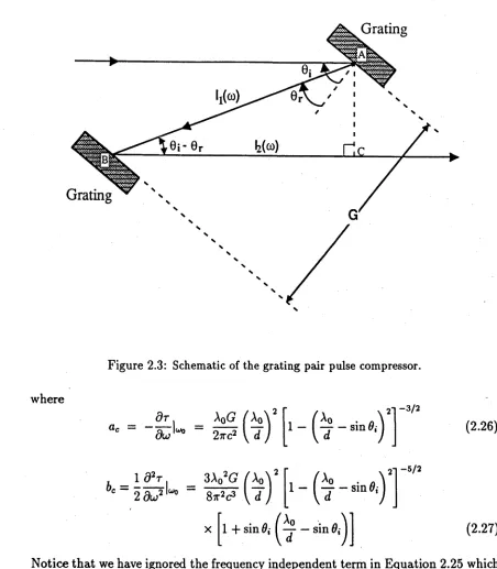
According to Figure 2.3, the optical length I = li + l2 can be expressed as [7]

l(u>) = G[sec9r(u>) + cos 0,- + sin 0, tg9r(u)\ (2.23)

where G is the perpendicular distance between the gratings, 0, and 9r are the incident and diffraction angles which satisfy the grating equation for first order diffraction:

sin0; -f sin0r(u;) = — (2.24)

a

where d is grating constant.

Substituting Equations 2.23 into 2.22 and expanding r at lj0 to second order, we

get [7]

(25)

Grating

Grating ^

Figure 2.3: Schematic of the grating pair pulse compressor.

where

dr

d r = —

A0G / a0\ 2 i r c ^ \ d )

1d2r _ W G ( X 0\

2 du2 iw° “ V d )

1 -f sin Oi

1 — — sin Oi

1 — f — — sin Oi

21

( y - s i n ö . )

- 3 / 2

- 5 / 2

(2.26)

(2.27)

Notice that we have ignored the frequency independent term in Equation 2.25 which simply induces an overall delay but does not affect the pulse envelope. Finally, the phase shift can be obtained by integrating Equation 2.25 with respect to u;. The result is, after ignoring the constant phase shift,

1 2 1 3

$ c(u) = —- a c(u;-Wq) + - b c(u>-LJ0) (2.28)

[image:25.549.54.506.48.565.2]

(26)

where

a =

1 + sin — sin Oij

i - ( 4 - s in 0 - ) 2 These are the desired results.

(2.30)

2.2.2 M odelling a P ulse C om pressor

A grating pair through which an optical pulse is passed simply causes a frequency

dependent phase shift $ c, so the process of the pulse compression can be is easily

modelled in the frequency domain. If we assume that the Fourier transform of the

input pulse is:

U(io) = \U(u)\ exp[i$(u;)] (2.31) then the Fourier transform of the compressed pulse can be expressed as:

Vc(u) = \U(u)\ exp {i [$ (cj) + $ c(u;)]} (2.32) Finally the envelope of the compressed pulse is determined by the inverse Fourier

transform of Equation 2.32:

1 f+°°

= — / |Cf(w)| exp {i [$(u/) 4 * c(u>)]} e x p ( -2wt) du (2.33)

Ideally, if 3>(u;) 4 <I>c(u;) = 0 (which means that the frequency chirp of the input

pulse is exactly cancelled after it passes though the grating pair), the envelope of

compressed pulse is just given by the Fourier transform of the power spectrum of

the input pulse. In this case, the pulse duration A tf whm of the compressed pulse is

the minimum available given by the transform-limit.

In the real situation, the frequency chirp on the output pulse from a fiber can

not be exactly cancelled by the gratings. Fortunately, the pulse emerging from a

fiber contains close to a linear chirp over most of the pulse width (see Figure 2.2(h)).

In this region, the phase shift can be written as

$(w ) = i ap(u - u 0)2 (2.34)

where av is the chirp parameter which is equal to the inverse of the slope of the

(27)

separation between the gratings so that the linear group delay term of Equation 2.25 (corresponding to the quadratic phase shift in Equation 2.28) cancels the linear chirp on the pulse, it is possible to compress the pulse close to the transform-limit under the conditions where the second-order group delay in the compressor is sufficiently small.

Therefore, the optimum condition for the pulse compression is normally defined as [101]

- uq)2 ~ 0 (2.35)

where 4>(u>) is expressed in Equation 2.34. This condition can be met by adjusting the grating separation to make ac = ap. Theoretically, av can be obtained by making a least-squares fit of the linear function of u:(t) in the linearly frequency chirped region. Experimentally, it can be estimated by A f/^m /A u;, where At f whm

and Au are the measured duration and spectral bandwidth of the pulse emerging from the optical fiber.

2.2.3 T he Effect of th e Cubic P h ase Shift

An optical pulse containing a linear frequency chirp can be compressed by a parallel grating pair. This occurs because the compressor induces a frequency dependent phase shift on the optical pulse as it passes through. In the small bandwidth limit, the phase shift can be expressed as a quadratic function of frequency, which will exactly cancel a linear frequency chirp on the input pulse and generate a bandwidth- limited compressed pulse. For large bandwidth, however, an additional cubic term becomes important and must be added to the relation between the phase shift and frequency, and it can cause additional pulse broadening and asymmetry in the pulse shape [58].

(28)

frequency with time is assumed so that its electric field can be written:

E(t) ~ exp

- 2 i n 2 l 4 ' 21 exp < —i a ’0< +

5<^)<2

(2.36)

where T0 is the pulse duration, u;0 is centre carrier frequency, and ßc is the chirp parameter.

The Fourier transform of the electric field is

E( u) ~ exp - 2 In 2 LJ —_WoV

Aujh ) exp i —2 Au V — Wn)2}

Where A i s the frequency bandwidth which satisfies the relation:

(2.37)

AwtT0 = ^/(4 In 2 )2 + /J? (2.38)

According to Equation 2.32, the Fourier transform of the compressed pulse can be expressed as:

E e(u>) ~ exp - 2 In 2 /<*> - c jqV

v“ä ^t )

exp [i^(a;)] (2.39)

where

+ *«(“') (2-4°)

and 4>c is the phase shift induced by the grating compressor as the pulse propagates through it, which is given by Equation 2.29. Substituting Equation 2.29 into 2.40 leads to:

=

\£$u

-

“ ° )2 ■

W“ -

w° )2 ( 1 - ( 2 -4 i )

where a is given by Equation 2.30.

For the optimum compression, the quadratic phase shift of the pulse compressor exactly cancels the phase of the linearly chirped pulse. This requirement can be satisfied by taking:

ac = ft/A w ? (2.42)

In this case, Equation 2.41 can be written:

(29)

Note that the duration of the chirped pulse before compression is much greater than the transform-limited value, that is, Au^To > > 4 In2. From Equation 2.38, therefore, ßc « AcobT0. Substituting this result in Equation 2.43 leads to

(2«>

where

C„ = To2 45j(

is a dimensionless constant dependent on the input pulse and grating parameters.

The compressed pulse in the time domain can be obtained by substituting Equa tion 2.44 into 2.39 and then taking the inverse Fourier transform. The result is

Ee(t) ~ exp(-iioot)

J

exp(—21n2A i^) exp ( i^ C nA v* ^

x exp(—i27rAi/n/t„/) d(Ai/„/) (2.46)

where tni = Avt,t, and A vni = (u; — u o )/Alji, = (u — i/o)/Ai/j,.

Figure 2.4 shows the intensity profile of the compressed pulse calculated from Equation 2.46 for Cn — 0 (dashed line) and Cn = 10 (solid line). For the case Cn = 0,

Figure 2.4: The normalized intensity of the compressed pulse as a function of time for

(30)

the compressed pulse has a transform-limited Gaussian shape and maximum peak

power. For the latter case, the pulse is evidently broadened and the peak power

is dramatically reduced. In addition, the peak of the pulse is shifted toward the

trailing edge, the envelope is asymmetric and it has along, oscillating tail.

To understand how Cn affects the compressed pulse duration and peak intensity,

the time-bandwidth product A VbTfwhm and the normalized peak intensity \An/Ao\2

of compressed pulse are plotted as function of Cn in Figure 2.5. As is evident, the

time-bandwidth product increase from 0.44 for Cn — 0 to 0.71 for Cn = 10. This is

accompanied by a decrease in the peak intensity from 1 to 0.54.

T3 0.5

Figure 2.5: The time-bandwidth product (solid line) and the normalized peak intensity

(dashed line) as functions of Cn.

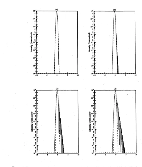
Figure 2.6 give the pulse shapes for different values of Cn = 0.5, 1, 2, and 3.

For Cn = 0.5 (see Figure 2.6(a)), A VbTfwhm = 0-45 and |i4n/A 0|2 = 0.98. The

compressed pulse remains Gaussian. For Cn = 1 (see Figure 2.6(b)), A VbTfwhm —

0.47 and |An/A o|2 = 0.95 and the pulse shape is still quite close to Gaussian. As

Cn increases to 2 (see Figure 2.6(c)), A VbTfwhm — 0-51 and \An/ A 0\2 = 0.87. As is

(31)

Figure 2.6: Comparison between the compressed pulse profile for Cn = 0 (dashed line)

[image:31.549.41.524.77.645.2]

(32)

As Cn increases further to 3 (see Figure 2.6(d)), A v^T j^m = 0.54 and |An/Ao|2 = 0.80 and more energy feeds into the oscillating tail significantly reducing the peak intensity.

According to above results, Cn < 1 can be used as a criterion for obtaining a high quality compressed pulse. In this condition, the compressed pulse has a very close to bandwidth-limited duration, high peak intensity and good shape. Alternatively, the criterion can be written as follows by using Equation 2.45

TpAuja < ^ u>o

As an example, to obtain a 1 ps pulse at 1.053 /im wavelength, A v = 16.4 Ä is required. If the linearly frequency chirped pulse to be compressed has a Gaussian envelope and duration To = 100 ps, then Equation 2.47 is satisfied if a < 2.3.

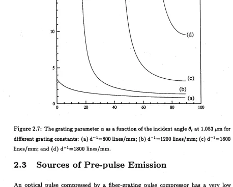
In Figure 2.7, the values of a are shown as a function of the incident angle

Si for different grating constants at a wavelength of 1.053 /im. As can be seen, for 1/d = 1800 lines/mm it is very difficult to obtain values of a below 10 and, hence, such gratings are far from optimal. Theoretically, a smaller 1/d is better, however, the grating separation increases rapidly as 1/d decreases for a given ac

(see Equation 2.26). Hence too small a value of 1/d will lead to impractically large grating separations. Therefore, a trade-off exists between the grating separation and the “quality” of the compressed pulse. In the above example a grating with 1/d = 1200 lines/mm provides a good trade-off. To satisfy a < 2.3, the incident angle is chosen so that Si > 40°.

In this section, a simple and practical criterion has been developed to assist in the design of a compressor based on a simple model which assumes that the pulse to be compressed has a Gaussian shape and a linear dependence of frequency with time. Notice that although the criterion is developed specifically for a grating pulse compressor, the results can also be applied to other types of compressor, such as a prism pair [70], prism-gratings [6], and acousto-optic light deflectors [71], etc. It is only necessary to substitute an appropriate expression for a for the particular compressor under consideration for the above results to be applicable.

(33)

Figure 2.7: The grating parameter a as a function of the incident angle 0, at 1.053 /im for

different grating constants: (a) d-1 =800 lines/mm; (b) d-1 = 1200 lines/mm; (c) d-1 = 1600

lines/mm; and (d) d -1 = 1800 lines/mm.

2 .3

S o u rces o f P r e -p u lse E m issio n

An optical pulse compressed by a fiber-grating pulse compressor has a very low intensity contrast ratio (the ratio of the peak intensity to the pre-pulse intensity). In the following study, numerical simulations will be used to identify the sources which cause the pre-pulse emission.

In the simulations, the parameters that have been used are listed below.

INPUT PULSE PARAMETERS: Wavelength: A = 1.053 /zm

Pulse shape: u(£,t/T0) = Asech(l.76t/T0)

Pulse duration: To = 35 ps Peak power: Pq = 50 W FIBER PARAMETERS:

Fiber core material: fused silica

[image:33.549.54.512.73.441.2]

(34)

Linear refractive index: n0 = 1.45

Nonlinear refractive index: n2 = 1.22 x 10“22 (m /V )2 GVD: D = 30 ps/nm /km

Loss: 7 = 0

Effective core area: Aeff = 4.5 x 10~7 cm2 Fiber length: 1 km

For the above parameters, z0 = 1.09 x 105 m, Pi = 3.43 x 10-3 W and A = 121. Calculations of the output from the fiber are shown in Figures 2.8 and 2.9. As is evident from Figure 2.8(a) the output pulse is transformed from sech2 to rectangular in time and develops some intensity modulations close to the leading and trailing edges. In frequency space (see Figure 2.8(b)), the main part of the pulse (region

A) has a linear dependence of frequency with time. Near the edges, however, there are two regions where the frequency oscillates, one at the extremes of the frequency region (region B and B'), and the other around the central frequency of the pulse (region C and C) . Figure 2.8(c) shows the spectrum of the pulse. As can be seen, the spectrum has a, square shape with sidelobes corresponding to the regions where the frequency changes nonlinearly (region B and B' in Figure 2.8(b)). The spectrum has bandwidth of about 35 Ä.

Figure 2.9(a) shows the compressed pulse under the optimum compression con ditions and with a = 3.0. The compressed pulse duration is 0.90 ps, corresponding to time-bandwidth product of 0.88 which is close to the bandwidth-limit for a rect angular pulse of 0.83. Figure 2.9(b) shows, using a log scale, the compressed pulse (solid line); the pulse launched into the fiber (dashed line); and the pulse emerging from the fiber (dashed-dot line). Evidently, the contrast ratio of compressed pulse is very poor. After compression, the linearly chirped region A in Figure 2.8(a) forms the main pulse; the region B and B' produce the pre-pulse and post-pulse; and region C and C give the low intensity wings.

Note that the spectrum of the pulse emerging from the fiber has a rectangular envelope which is not an ideal shape for compression. From Equation (2.33), for ideal

/

compression conditions, 4>(u;) + = 0, the compressed pulse vc(t) is just the

(35)

H 100

t/T0

(O-CÖq)Tq

Figure 2.8: (a) The intensity of the output pulse from the fiber as a function of time; (b)

the instantaneous frequency of the pulse as function of time; and (c) the power spectrum

(36)

Figure 2.9: The intensity of the compressed pulse as a function of time: (a) linear scale,

and (b) log scale. In the latter the pulse launched into the fiber (dashed) and that emerging

(37)

Fourier transform of the envelope of the spectrum \U(u>)\. Therefore, a rectangular spectral shape alone will lead to the formation of a slowly decaying oscillating tail on the compressed pulse. In Figure 2.9(a), the fast intensity oscillations appearing on either side of the main pulse arises primarily due to the rectangular spectral shape.

From the above simulation results, it can been concluded that there are three major sources that cause the pre-pulse emission: (a) the rectangular spectral shape leads to a slowly decaying oscillating tail on both sides of main compressed pulse; (b) the nonlinearly frequency chirped light leads to the formation of a subsidiary peak on the compressed pulse on both sides of the main pulse located around t = T0/2 to T0 from the main pulse; (c) the frequency unshifted light forms low intensity wings which appears at t > ±T 0.

2.4 N um erical m odelling o f C ontrast Enhancem ent

by Spectral Shaping

A simple method to improve the intensity contrast is to remove the nonlinearly chirped components from the frequency spectrum and smooth the spectral shape [77]. In this section, we will numerically model the contrast enhancement achieved by using such a spectral shaping method.

Before starting the detailed study, it is necessary to know what the ideal spectral shape for compression actually is. It has been shown in the previous section that, in an ideal compression condition, the compressed pulse is simply the Fourier transform of the power spectrum (see Equation 2.33). In order to obtain an ideal Gaussian shape for the compressed pulse, a Gaussian-shaped spectrum is, therefore, required. As we deduced from the previous section, the spectrum of the pulse at the output of the fiber has a “square” shape. Thus a Gaussian-shaped bandpass filter can be used to re-shape this spectrum into a Gaussian profile.

(38)

G aussian-shaped bandpass filter has following form:

T,(ui) = T,o exp 2 In 2 (2.48)

where Tao is th e m axim um transm ission, Au>9 is th e FW HM of th e power transm is

sion.

A fter spectral shaping, from E quation 2.33, the compressed pulse can be de

scribed by

1 r +°°

vc(£) = — / Ta(u) \U(uj)\ exp {i [$(u>) + $ c(u>)]} ex p (—icot) du. (2.49)

2ttj— oo

In th e following calculations, we use th e sam e laser and fiber param eters as those

in Section 2.3, and th e m axim um spectral transm ission Ta0 = 1. Figure 2.10(a) shows

th e calculated sp ectra after spectral shaping by using the filters w ith AAa = 15 Ä

(solid curve) and AAa = 9 Ä (dashed curve) (AAa = A2Au;a/(27rc)). Figure 2.10(b)

shows th e corresponding compressed pulse shapes.

For AAa = 15 Ä, th e spectrum has been shaped from th e square to a near

G aussian profile, and th e compressed pulse has a dom inant short pulse and long pre-

and post-pulses arising from th e frequency unshifted light. The m ain pulse duration

is 1.2 ps. T he tim e-bandw idth product of th e compressed pulse is 0.49, close to the

tim e-bandw idth product for a G aussian pulse. As is evident, th e intensity contrast

is improved after th e spectral shaping, and is > 103. T he m ain compressed pulse is

a good fit to a G aussian profile over three orders of intensity. Since the nonlinearly

chirped frequency com ponents are not to tally removed, they are still apparent on

either side of th e spectrum at relatively low intensities after spectral shaping with

AAa = 15 Ä. They result in th e form ation of rapidly oscillating intensity regions

near th e m ain compressed pulse.

A fter spectral shaping using bandpass filter w ith AAS = 9 Ä, th e spectrum now

has a G aussian profile, and th e compressed pulse has a duratio n of 1.8 ps, which

is th e exact transform lim it of a 9 Ä G aussian spectrum . In this case, th e main

compressed pulse can be fitted w ith a G aussian profile over six orders, although the

pre- and post- pulses due to th e unshifted frequency com ponents are still present.

(39)

Figure 2.10: (a) The spectral shape after spectral shaping with A A = 15 Ä (solid curve)

(40)

2 5

Figure 2.11: (a) The pulse shape of the pulse emerging from a fiber, (b) the compressed

pulse shape, dashed curve: z=0.5 km; dashed-dot curve: z=1.0 km; solid curve: z=1.5

(41)

Spectral shaping can change th e spectrum to the required shape and can remove

th e energy from th e nonlinearly chirped frequency com ponents very efficiently, but

it cannot directly remove th e low intensity wings at th e central frequency (see Figure

2.10(b)). However, optical wave breaking can transfer th e energy from the unshifted

frequency com ponents in th e leading and trailing edges of th e pulse, to extreme

frequencies. The longer th e fiber, th e more energy will be transferred in this way.

Hence, th e combined use of a long fiber and a spectral filter can reduce the intensity

of th e unshifted frequency com ponents and therefore their corresponding pre- and

post- pulses.

Figure 2.11(a) shows th e pulse shapes at th e fiber o u tp u t for various fiber lengths

(dashed curve: z=0.5 km; dashed-dot curve: z = l km; and solid curve: z=1.5 km),

while Figure 2.11(b) gives the compressed pulse shapes after spectral shaping with

A A = 9 Ä. T he compressed pulses have th e same pulse durations of 1.8 ps (transform

lim it of th e G aussian spectrum ). As is clearly shown in th e figure, however, the

co n trast of the compressed pulses increases w ith th e increasing fiber length.

However, there is a lim it on the reduction of th e intensity of th e unshifted fre

quency com ponents th a t can be achieved by increasing th e fiber length. In the above

exam ple, th e o u tp u t pulse from th e fiber already has a square shape w ith a very

flat to p for a 1 km fiber (see Figure 2.11(a)). This m eans th a t, if th e fiber length

is fu rth er increased, self-phase m odulation will be much less efficient in increasing

th e frequency in th e m ain linearly frequency chirped region, w hilst it is still very

efficient in transferring energy from th e sharp leading and trailing edges to extrem e

frequencies. This results in a reduction of th e bandw idth at 1.5 km com pared with

th a t at z = l km (see Figure 2.12). If th e fiber is too long, th e pulse duration at the

o u tp u t of th e fiber will also increase m arkedly due to GVD, b u t not the bandw idth.

In th is case, a large gratin g separation would be required to compress such an outp u t

pulse from th e fiber, an d this m ay be im practical in some lab o rato ry experim ents.

(42)

1500

la looo £* '53

a £

a

13 500

b

l

3 600

t

's—*'

>>

a 4oo

13

b

iL

200

3 600

t

's—'

>% g 400 §

13

b

8

.

200

1 . . . . I . . . .

(C)

-L i i i 1. . .1

-300 -200 -100 0 100 200 300

( o > —o)q) Tq

Figure 2.12: The power spectra of the output pulse from the fiber with various lengths:

(43)

2.5 S u m m a ry

(44)

C hapter 3

C hirped P u lse A m plification and

C om pression

Chirped pulse amplification has become a standard technique for generating high power, ultra-short pulses. Until very recently, most of the CPA Ndiglass laser sys tems were based on the fiber-grating pulse compression scheme to generate ultra- short pulses starting with a relatively long pulse, because alternative laser oscillators which could generate pulse durations < 1 ps at ~ 1 fim such, as the additive-pulse mode-locked (APM) laser [92] were still in the stage of laboratory study. For many applications of CPA lasers such as the study of ultra-short laser pulse interaction with matter, a high intensity contrast ratio is essential. Due to the poor inten sity contrast ratio associated with a normal fiber-grating pulse compression scheme, the elimination of the pre-pulse emission is a major problem when developing such systems.

In this chapter, an experimental study of a fiber-grating pulse compression sys tem using chirped pulse amplification will be presented. Using the spectral shaping technique, an intensity contrast > 103 has been achieved in our CPA leiser.

(45)

follow-ing sections. Section 2 describes the CPA laser system developed at the Australian National University (ANU). Section 3 presents the experimental studies the spectral shaping technique for lowering the pre-pulse levels. Section 4 discusses the experi mental results on the chirped pulse compression. A brief summary is finally given in Section 5.

3.1 Measurements of the Duration of Ultra-Short

Pulses

Optical pulse measurements can be divided into direct and indirect methods. The current generation of the streak cameras, the fastest tools for direct meetsurements, have time resolutions around 1 ps. As the pulse duration shortens into the femtosec ond range, direct measurements become very difficult or are impossible. However, the duration of femtosecond pulses, as well as picosecond pulses, can be determined indirectly by the measurement of their intensity (or interferometric) autocorrelation functions by means of some nonlinear optical techniques, such as second harmonic generation (SHG) [109], two photon fluorescence (TPF) [28], and degenerate four wave mixing (DFWM) [88], etc.

In the infrared and visible frequency range, SHG in a nonlinear medium is the most popular method for pulse duration measurements, because it can sup ply very high time resolution [26]; give “background free” measurements [109]; and be adapted for use with single pulses [42]. Therefore, it is very suitable for measuring pulses from a Nd leiser and its second harmonic (SH) frequency.

(46)

Beam Splitter

SHG Crystal Filter

Detector

Aperture

Variable Delay

Figure 3.1: The layout of the CW autocorrelator.

3.1.1 T heoretical Background to A utocorrelators

The spatial length of an optical pulse is given by lp = cT0, where c is the speed of light in vacuum and To is the pulse duration. For a pulse duration T0 = 1 ps, the spatial length of the pulse is lp = 0.3 mm which is an easy distance to measure if we can transfer the measurement from the time to space domain. This is the basic idea underlying the measurement of ultra-short pulse durations using an autocorrelator.

(47)

direction of the SH beam satisfies the phase matching condition

k£w = ky + kSf (3.1)

where k" and k£ are the wave vectors of the two incident pulses, and k ^ is the wave vector of the SH pulse. For small signal conversion, the instantaneous intensity of the SH signal is proportional to I(t)I(t — r). Since the response time of the detector is much longer than the pulse duration, the recorded SH signal 5 (r) is proportional to the time integral of the intensity, i.e. the intensity autocorrelation G(t) [45]

S(t) oc r I(t)I(t - r)dt = G(t) (3.2)

J—oo

To determine the pulse duration from the recorded signal 5 (r), the recorded signal S(t) should be first normalized. From Equation 3.2, one can obtain

S(t)/S(0) = G (r)/G (0) (3.3)

which shows that the normalized recorded signal is actually the normalized intensity autocorrelation function. If the pulse shape is known, the pulse duration (FWHM of the intensity) can be calculated from a measurement of the width Ar0 (FWHM of the G(t)) of the autocorrelation function.

Table 3.1: The ratios between the FWHM (A r0) of the pulse

autocorrelation function and the pulse duration (To), and the time- bandwidth product for three given pulse shapes.

Pulse Shape

Aro/To

A uTq

m = '

1 if 0 < t< 0 otherwise

1 0.886

I(t) = exp[—4 In 2(f/T0)2] 1.414 0.441

I(t) =sech2(1.7 6t/T0) 1.55 0.315

(48)

shapes. The bandwidth-time product can be used to check whether the measured pulse is equivalent to its transform limited duration. If the pulse shape is unknown, it is necessary to fit the autocorrelation curve numerically using the pre-assumed pulse shape.

For high energy laser systems, the repetition rate is limited to a few pulses per second (or less). In this instance, the above autocorrelator arrangement is inconve nient because it would be very time consuming to record the whole autocorrelation trace. In addition, the energy jitter of the pulse between each shot would reduce the accuracy of the measurement. To overcome these problems, a single pulse mea surement technique has been developed [36, 42] based on the idea of imprinting the autocorrelation signal on the transverse intensity distribution of the SH beam. The SH signal is then recorded by a detector array which images this distribution. Thus, a whole autocorrelation trace can be recorded from one single pulse.

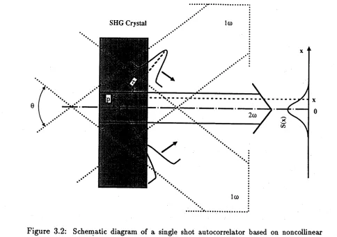
Figure 3.2 show the schematic diagram of a single shot autocorrelator based on the NSHG technique. Two incident pulses are generated by a beam splitter and intersect in the SHG crystal at an angle <j>. Let us assume that the beam diameter

Df, is large compared with the spatial length of the light pulse, lp =cTo, so that the intensity distribution of the beams normal to the direction where the SH is emitted is uniform in the region where the pulses overlap. Let the two incident pulses have the same temporal intensity profile I(t), and the SH signals have a spatial distribution

S(x) (assuming x=0 at the centre of SH beam). It can be simply demonstrated [86] that the relative delay of the incident pulses interacting in the crystal is independent of the y position for a fixed x. Hence, the instantaneous intensity of the SH pulse at any point for a given x is proportional to I(t)I(t — r) with the relative delay r given by

2sin(^>/2) ---x

V9

(3.4)

where vg is the group velocity of the incident pulse in the crystal. Using a slow detector response, the recorded signal is proportional to the time integral of the SH intensity, i.e., the intensity autocorrelation G(r)

S(x) oc

f

— r)dt = G(t).

J—oo

(49)

SHG Crystal

Figure 3.2: Schematic diagram of a single shot autocorrelator based on noncollinear second harmonic generation.

Let AXo be the FWHM of the recorded signal 5(x). The autocorrelation width A r0 can be obtained from Equation 3.4

2sin(0/2)

A To = --- -Ax0. (3.6)

V9

To determine the absolute value of A r0 from Equation 3.6, it is necessary to know the exact values of the angle (f> and the group velocity vg. However, there is a very simple and practical method for calibrating the autocorrelator [86]. When a time delay A7i is added to one of the incident pulses, the recorded signal will be

S(x + A xi), i.e., the whole of the SH trace 5(x) will be shifted by Axi along the x axis. From Equation 3.4, one can obtain

Arx 2sin(0/2)

Axj vg

Substituting this result into Equation 3.6 yields

(3.7)

[image:49.549.39.523.54.395.2]

(50)

The pulse duration can be the determined from the measured A tq using the same

method as that discussed in the earlier part of this section.

3.1.2 CW A utocorrelator

The experimental layout of the CW autocorrelator is shown in Figure 3.3. The beam

Variable Delay Unit 2

M3 Beam Splitter

Filter Photomultiplier

Aperture

PI • P3 : Prism Ml • M4: Mirror

Variable Delay Unit 1 X-Y Recorder Oscilloscope

Figure 3.3: The experimental arrangement of the CW autocorrelator.

splitter produced two replicas of the incident pulse (train), which passed through the variable delay units 1 and 2, respectively. The two pulses were then directed parallel, but not collinear, and focused by a lens (focal length = 1 3 0 mm) into a SHG crystal (LÜO3, 1 mm thick). The SH signal was generated at the angle bisecting that between the two fundamental beams, and was detected by a photomultiplier. A green bandpass filter in front of the photomultiplier was used to suppress the light scattered from the fundamental beam and other undesirable frequencies. The output signal from the photomultiplier was recorded on either a X-Y recorder or an oscilloscope depending on which variable delay unit was used.

(51)

(0.025mm/step) at a speed of 10 step/s or 100 step/s via a pantograph to reduce the step distance by ratios of 1:1, 2:1, 5:1, 7.5:1, 10:1 or 20:1. The maximum delay that could be provided by this unit was ±300 ps. The SH signal was detected by the photomultiplier and then recorded on an X-Y recorder.

In the delay unit 2, the variable delay was provided by a rotating prism driven by a motor at 1800 rpm. The input beam was retroreflected by the rotating prism P2 with a horizontal displacement, then the stationary prism P3 reflected the beam back to P2 but with a vertical displacement. The beam reflected again by P2 emerged parallel to the incident beam but displaced below it. A mirror M3 placed under the incident beam further reflected the beam in the required direction.

When the path length of the variable delay unit 1 is adjusted such that the time delay of two incident pulses in the crystal is zero at 9 = 0 (see Figure 3.4), it can be shown that the relative delay between the two incident pulses at the entrance to the crystal is given by

r 4/,g(Q

c

for a small angle ( — 10° < 0(t) < ±10°). In Equation 3.9 6 is in radians.

When the prism P2 rotates at a constant angular speed, the time delay introduced

(52)

3 0.5

Time Delay

Figure 3.5: The measured autocorrelation trace, where the delay unit 1 is used for gen erating the delay.

by this delay unit varies linearly with time. The maximum delay depends on lp and the maximum usable angle of 6 for the total internal reflection to occur in the prism. In our experiments, the maximum usable angle was 6 < ±5.2°, and lv = 75 mm, so the maximum delay, was about ± 1 8 0 ps.

The compressed CW mode-locked Nd:YLF laser pulses were used to test the autocorrelator. The pulses had the duration of ~ 1 ps at a repetition rate of 76 MHz (see Section 3.2). The measured autocorrelation trace of these pulses is shown in Figure 3.5, where the delay unit 1 was used to introduce the delay. The FWHM of the autocorrelation trace was A r0 = 1.1 ps, and the corresponding pulse duration was 0.7 ps, assuming a sech2 pulse shape.

(53)

KDP Crystal _Polarizer

Figure 3.6: Schematic of double pulse generation from a single pulse.

Figure 3.6 shows the experimental arrangement for double pulse generation from a single pulse. Due to double refraction in KDP crystals, a linearly polarized input pulse is split into the two crossed, o- and e-polarized pulses, and they travel at their respective group velocities through the crystal (in a KDP crystal the e-pulse travels faster than the o-pulse). The output pulses from the crystal have a relative time delay of At = Lc\l/v° — l/v j|, where Lc is the crystal thickness, v° and vg

are the group velocities of the o- and e- pulses, respectively. By passing the pulses through the polarizer, it is possible to generate a linearly polarized double pulse as is required.

(54)

x=-A t

Figure 3.7: An illustration of a double pulse autocorrelation trace.

Figure 3.8(a) shows the autocorrelation trace of the double pulses recorded by the oscilloscope. In the experiment, a 2.5 cm KDP crystal, cut at 59.2° between the normal of the crystal surface and the optic axis, was used to produce the twin-pulses. When the beam was close to normal incidence, the group velocities of the o- and e- pulses were v° = 1.9664 x 108 m /s and v' = 2.0188 x 108 m /s at 1.053 fim (see Table 4.1 in Chapter 4). Hence, the output pulses from the crystal were separated by A t =3.30 ps. From Figure 3.8(a), the calibration constant was 2.44 ps/10 fis.

Note that the calibration can also be performed by inserting a glass plate of known thickness into one of the beams. The advantage of the double pulse technique is that it is free of the errors caused by the trigger jitter in the measurement system.

Development of a high contrast Nd:glass laser using chirped pulse amplification