This is a repository copy of
Sparse model identification using a forward orthogonal
regression algorithm aided by mutual information
.
White Rose Research Online URL for this paper:
http://eprints.whiterose.ac.uk/1970/
Article:
Billings, S.A. and Wei, H.L. (2007) Sparse model identification using a forward orthogonal
regression algorithm aided by mutual information. IEEE Transactions on Neural Networks,
18 (1). pp. 306-310. ISSN 1045-9227
https://doi.org/10.1109/TNN.2006.886356
[email protected]
https://eprints.whiterose.ac.uk/
Reuse
Unless indicated otherwise, fulltext items are protected by copyright with all rights reserved. The copyright
exception in section 29 of the Copyright, Designs and Patents Act 1988 allows the making of a single copy
solely for the purpose of non-commercial research or private study within the limits of fair dealing. The
publisher or other rights-holder may allow further reproduction and re-use of this version - refer to the White
Rose Research Online record for this item. Where records identify the publisher as the copyright holder,
users can verify any specific terms of use on the publisher’s website.
Takedown
If you consider content in White Rose Research Online to be in breach of UK law, please notify us by
Sparse Model Identification Using a Forward Orthogonal Regression Algorithm Aided by Mutual Information
Stephen A. Billings and Hua-Liang Wei
Abstract—A sparse representation, with satisfactory approximation ac-curacy, is usually desirable in any nonlinear system identification and signal processing problem. A new forward orthogonal regression algorithm, with mutual information interference, is proposed for sparse model selection and parameter estimation. The new algorithm can be used to construct parsi-monious linear-in-the-parameters models.
Index Terms—Model selection, mutual information, orthogonal least squares (OLS), parameter estimation.
I. INTRODUCTION
The central task in learning from data is how to identify a suit-able model from the observational data set. One solution is to con-struct nonlinear models using some specific types of basis functions, aided by various state-of-the-art techniques [1]–[5]. Among the ex-isting sparse modeling techniques, linear-in-the-parameters regression models, which will be considered in this letter, are an important class of representations for nonlinear function approximation and signal pro-cessing. A general routine for linear-in-the-parameters modeling often starts by constructing a model term dictionary, whose elements are the candidate model terms. The task of system identification involves two aspects: the selection of the significant model terms and the determina-tion of the number of model terms involved in the final identified model. The objective is to obtain a satisfactory sparse representation that in-volves only a small number of model terms by making a compromise between the approximation accuracy and the model complexity (model size). Notice that the objective of dynamical modeling is not merely data fitting. In dynamical modeling, the resulting sparse model should fit the observational data accurately, but at the same time the model should be capable of capturing the underlying system dynamics car-ried by the observational data, so that the resulting model can be used in simulation, analysis, and control studies.
Many approaches have been proposed to address the model struc-ture selection problem; most of these focus on which bases are signifi-cant and should be included in the model. The orthogonal least squares (OLS) algorithm [2], [6], [7], which was initiated for nonlinear system identification, has become popular and has been widely used for sparse data modeling. This type of algorithm is simple and is very efficient at producing parsimonious linear-in-the-parameters models with good generalization performance [8]. An advantage of the OLS-type algo-rithms is that commonly used model selection and regularization tech-niques, for example the Akaike information criterion (AIC), Bayesian information criterion (BIC), and generalized cross validation (GCV) [9]–[11], can easily be adopted and incorporated into the model struc-ture selection algorithms to yield compact linear-in-the-parameters re-gression models with good generalization properties [12]–[14].
Manuscript received March 30, 2006; revised July 10, 2006. This work was supported by the U.K. Engineering and Physical Sciences Research Council (EPSRC-UK).
The authors are with the Department of Automatic Control and Systems Engineering, the Univerity of Sheffield, Sheffield, S1 3JD, U.K. (e-mail: [email protected]; [email protected]).
Color versions of one or more of the figures in this paper are available online at http://ieeexplore.ieee.org.
Digital Object Identifier 10.1109/TNN.2006.886356
In the OLS-type algorithms, the criterion that is used to measure the significance of the candidate bases (model terms) is the error reduc-tion ratio (ERR), which is equivalent to the squared correlareduc-tion coef-ficient and is similar to the commonly used Pearson correlation func-tion. Experience has shown that the OLS algorithms interfered by the ERR criterion can usually produce a satisfactory sparse model with good generalization performance. The adoption and the domination of the ERR criterion, however, does not exclude other criteria. It follows from practical experience that the selected model subsets are often cri-terion-dependent.
In this letter, a new criterion, derived from mutual information, is adopted into the OLS algorithm to measure the significance of candi-date bases and to interfere with the model subset selection. The moti-vation of the adoption of a mutual information criterion is based on the following considerations. It is known that the task of modeling from data is generally structure-unknown and the model term dictionary is often predetermined and thus fixed. For this case, the selected model structures are usually criterion-dependent. This implies that the mutual information criterion and the ERR criterion may or may not produce exactly the same model structure given the same modeling problem. The two criteria can be used in parallel, and the performance of the resultant models can then be compared. The model with the better per-formance will be chosen as the final model. In this manner, the two criteria will complement each other and thus produce a better model.
II. LINEAR-IN-THE-PARAMETERSREPRESENTATION
Consider the identification problem for nonlinear systems givenN pairs of input–output observationsfu(t); y(t)gNt=1. Under some mild conditions, a discrete-time nonlinear system can be described by the following nonlinear autoregressive with exogenous inputs (NARX) model [1]
y(t) = f(y(t01); . . . ; y(t0ny); u(t01); . . . ; u(t0nu))+e(t) (1)
whereu(t),y(t), ande(t)are the system input, output, and noise vari-ables,nuandnyare the maximum lags in the input and output, respec-tively, andf is some unknown nonlinear mapping. It is generally as-sumed thate(t)is an independent identical distributed noise sequence. The central task of system identification is to find a suitable approx-imatorf^for the unknown functionffrom the observational data. One solution is to construct nonlinear models using some specific types of basis functions including polynomials, kernel basis functions, and multiresolution wavelets [3]–[6], [15]. Among these existing modeling techniques, linear-in-the-parameters regression models, which will be considered in this letter, is an important class of representations for non-linear system identification, because compared to nonnon-linear-in-the-pa- nonlinear-in-the-pa-rameters models, linear-in-the -panonlinear-in-the-pa-rameters models are simpler to ana-lyze mathematically and quicker to compute numerically.
Letd = ny+ nuandx(t) = [x1(t); . . . ; xd(t)]T with
xk(t) = y(t 0 k);u(t 0 (k 0 n 1 k ny
y)); ny+ 1 k ny+ nu. (2)
A general form of the linear-in-the-parameters regression model is given as follows:
y(t) = ^f(x(t)) + e(t) =
M
m=1
mm(x(t)) + e(t)
= '''T(t) + e(t) (3)
whereMis the total number of candidate regressors,m(x(t)) (m =
1; . . . ; M)are the model regressors andmare the model parameters,
and'''(t) = [1(x(t)); . . . ; M(x(t))]T andare the associated
re-gressor and parameter vectors, respectively.
III. MUTUALINFORMATIONINTERFERENCE FOR
MODELSTRUCTURESELECTION
In the standard OLS algorithm [2], [6], [7], the significance of candi-date model terms is measured using the values of ERR, which is defined as the noncentralized squared correlation coefficient between two as-sociated vectors. This coefficient between two given vectorsxandy of sizeNis defined as
C(x; y) = (xTy)2 (xTx)(yTy) =
(N
i=1xiyi) 2
N
i=1x 2 i
N
i=1y 2 i
: (4)
Similar to the commonly used standard Pearson correlation coefficient, the function in (4) reflects the linear relationship between two vec-torsxandy. Both the standard Pearson correlation coefficient and the squared correlation coefficient in (4) have wide application in various fields.
Another useful criterion, derived from mutual information, can be used to measure the relationship of two random variables by calcu-lating the amount of information that the two variables share with each other. Mutual-information-based algorithms have in recent years been widely applied in various areas including feature selection [16]–[20]. In this letter, mutual information will be introduced to form a com-plementary criterion to the ERR criterion to interfere with the model structure selection procedure.
A. Mutual Information
Following [21], mutual information is defined as follows. Consider two random discrete variablesxandy with alphabetX and Y, re-spectively, and with a joint probability mass functionp(x; y)and mar-ginal probability mass functionsp(x)andp(y). The mutual informa-tionI(x; y)is the relative entropy between the joint distribution and the product distributionp(x)p(y), given as
I(x; y) = E log p(x)p(y)p(x; y)
=
x2X y2Y
p(x; y) log p(x)p(y)p(x; y) : (5)
The mutual informationI(x; y)is the reduction in the uncertainty ofy due to some knowledge ofxand vice versa. Mutual information pro-vides a measure of the amount of information that one variable shares with another. Ifyis chosen to be the system output (the response), and xis one regressor in a linear model,I(x; y)can be used to measure the coherency ofxwithyin the model.
B. Model Structure Selection With Interference of Mutual Information
Lety = [y(1); . . . ; y(N)]T be a vector of measured outputs atN time instants, and'''m = [m(1); . . . ; m(N)]T be a vector formed
by the mth candidate model term, where m = 1; 2; . . . ; M. Let D = f'''1; . . . ; '''Mgbe a dictionary composed of theM candidate bases. From the viewpoint of practical modeling and identification, the finite dimensional set D is often redundant. The model term selection problem is equivalent to finding a full dimensional subset Dn = f1; . . . ; ng = f'''i ; . . . ; '''i g ofn (n M) bases,
from the library D, where k = '''i , ik 2 f1; 2; . . . ; Mg and
k = 1; 2; . . . ; n, so thatycan be satisfactorily approximated using a linear combination of1; 2; . . . ; nas
y = 11+ 1 1 1 + nn+ e (6)
or in a compact matrix form
where the matrixA = [1; . . . ; n]is assumed to be of full column
rank, = [1; . . . ; n]T is a parameter vector, andeis the
approxima-tion error. The model structure selecapproxima-tion procedure starts from (3). Let r0 = y, and
`1= arg max
1jMfI(r0; '''j)g (8)
whereI(1; 1)is the mutual information defined by (5). The first signif-icant basis can thus be selected as1 = '''` , and the first associated
orthogonal basis can be chosen asq1 = '''` . Set
r1= r00 r T 0q1
qT
1q1q1: (9)
In general, themth significant model term can be chosen as fol-lows. Assume that at the(m 0 1)th step, a subsetDm01, consisting of
(m01)significant bases,1; 2; . . . ; m01, has been determined, and the(m 0 1)selected bases have been transformed into a new group of orthogonal basesq1; q2; . . . ; qm01via some orthogonal
transforma-tion. Let
q(m)j = '''j0
m01
k=1
'' 'T
jqk
qT
kqkqk (10)
`m= arg max
j6=` ;1km01 I rm01; q (m)
j (11)
where'''j 2 D 0 Dm01, andrm01is the residual vector obtained in
the(m 0 1)th step. Themth significant basis can then be chosen as
m= '''` and themth associated orthogonal basis can be chosen as
qm= q(m)` . The residual vectorrmis given by
rm= rm010r T m01qm
qTmqm qm: (12)
Subsequent significant bases can be selected in the same way step by step. From (12), the vectorsrmandqmare orthogonal, thus
krmk2 = krm01k20(r T m01qm)2
qT
mqm : (13)
By respectively summing (12) and (13) formfrom 1 ton, yields
y =
n
m=1
rT m01qm
qT
mqm qm+rn (14)
krnk2= kyk20 n
m=1
(rT m01qm)2
qTmqm : (15)
Notice that if the functionI(1; 1)in (8) and (11) is replaced by the squared correlation coefficient defined by (4), the above algorithm then belongs to the class of OLS-type algorithms [2], [6], [7]. The forward orthogonal regression algorithm interfered with mutual information will be referred to as the FOR-MI algorithm. The residual sum of squares,krnk2, which is also known as the sum-squared-error, or its
variants including the mean-square-error (mse), can be used to form criteria for model selection. There are many criteria used for model selection include the AIC, BIC, and GCV [9]–[11], [13]. One popular version for each of the three criteria is
AIC(n) = N log[mse(n)] + 2n (16) BIC(n) = N log[mse(n)] + n log(N) (17)
GCV(n) = N N 0 n
2
mse(n) (18)
where mse(n) = krnk2=N.
C. Parameter Estimation
It is easy to verify that the relationship between the selected original bases1; 2; . . . ; m, and the associated orthogonal bases
q1; q2; . . . ; qmis given by
Am= QmRm (19)
whereAm= [1; . . . ; m],Qmis anN 2 mmatrix with orthogonal
columnsq1; q2; . . . ; qm, andRmis anm 2 munit upper triangular matrix whose entriesuij(1 i j m)are calculated during
the orthogonalization procedure. The unknown parameter vector, de-noted bym = [1; 2; . . . ; m]T, for the model with respect to the
original bases [similar to (6)], can be calculated from the triangular equationRmm = gmwithgm = [g1; g2; . . . ; gm]T, wheregk =
rT
k01qk = qTkqk .
Note that some tricks can be used to avoid selecting strongly correlated model terms. Assume that at the(m 0 1)th step, a subset Dm01, consisting ofm 0 1significant bases1; . . . ; m01has been determined. Also assume that'''j 2 D 0 Dm01is strongly correlated
with some bases in Dm01, that is '''j is a linear combination of
; . . . ; m01. Thus, q(m)j T
q(m)
j = 0. In the implementation of
the algorithm, the candidate basis'''j will be automatically discarded
if q(m)j Tq(m)j < , whereis a positive number that is sufficiently small. In this way, any severe mullticolinearity or ill-conditioning can be avoided.
A similar algorithm, called maximally informative dimensions (MID), has been proposed in [20], where the main objective was to find, in a high dimensional stimulus space, significant features of sen-sory stimulus (“inputs”) that are most relevant to the measured neural responses (“outputs”). There is some similarity between FOR-MI and MID in that both algorithms employ the mutual information function to measure the dependency between two specified vectors. The implementation of the two algorithms, and the final objectives that the two algorithms aim to achieve, however, are different from each other. The FOR-MI algorithm deals with the linear-in-the-parameters regression problem, and involves a combination of a forward orthog-onal regression procedure and the calculation of mutual information. Significant bases are selected in a stepwise way, one at a time. The final objective is to produce a sparse regression model, where both the model structure and the unknown model parameters need to be determined using the OLS algorithm. The MID algorithm, however, is a nonlinear optimization method that uses a combination of gradient ascent and simulated annealing algorithms. The MID algorithm thus involves the calculation of not only the mutual information function itself but also the associated gradient. The MID algorithm aims to find the maximally informative dimensions in an iterative way by increasing the dimensionality until the information is saturated (up to the noise level). The unknown parameters in the model were estimated using some statistical approach.
IV. EXAMPLE
Fig. 1. Measurements of the solar wind parameterV Bsand theDstindex for the terrestrial magnetospheric system.
Fig. 2. GCV versus the number of regressors selected from the candidate model terms using both the OLS-ERR and the FOR-MI algorithms.
input, and theDstindex was treated to be the system output. The ob-jective here was to identify a mathematical model to forecast the future behavior of theDstindex. The data set was partitioned into two parts. The first 500 points were used for model estimation and the remaining 350 points were used for model performance test.
The polynomial NARX model was employed to describe the magnetospheric system. Denote the system input and output using u(t) = V Bs(t) and y(t) = Dst(t), respectively. The “input” vector for the model was chosen to bex(t) = [x1(t); . . . ; x12(t)]
[y(t 0 1); . . . ; y(t 0 5); u(t 0 1); . . . ; u(t 0 7)], and the candidate regressorsm(x(t))in (3) are of the formxij (t)xij (t)xij (t), where
xi
j (t) 2 fx1(t); . . . ; x12(t)g (k = 1; 2; 3), ik 2 f0; 1; 2; 3g,
0 i1+ i2+ i3 3, andjk 2 f1; 2; . . . ; 12g. Thus, a total of 455
candidate model terms are involved.
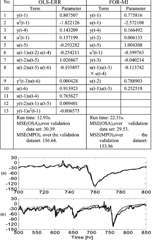
Both the OLS-ERR algorithm and the FOR-MI algorithm were ap-plied to the 455 candidate model terms. The associated criterion GCV is shown in Fig. 2, which suggests that the number of model terms included in the OLS-ERR and the FOR-MI identified NARX models should be 13 and 10, respectively. Note that the AIC and BIC produce similar results for this data set, and the curves for AIC and BIC were thus omitted. The selected model terms, along with the associated pa-rameter estimates are reported in Table I, where model terms are listed in the order of their significance (the order that the terms entered into the model). The FOR-MI identified model for this data set is in struc-ture simpler than the model produced by the OLS-ERR algorithm.
The performance of the two identified NARX models was inspected and compared by calculating both short-term and long-term predic-tions, over the validation data set. The performance of one-step-ahead (OSA) predictions and model predicted (MPO) outputs, calculated from the OLS-ERR and the FOR-MI identified models are presented
TABLE I
SELECTEDMODELSTRUCTURE BYOLS-ERRANDFOR-MI
Fig. 3. Prediction performance of the OLS-ERR and the FOR-MI identified models, over the validation data set, for the terrestrial magnetospheric system. (a) OSA predictions. (b) MPO. Thick solid line shows the measurements, thin solid line shows predictions from the OLS-ERR identified model, and thick dotted line shows predictions from the FOR-MI identified model.
in Table I and Fig. 3. Clearly, if mse is used as the criterion to measure the model performance, the FOR-MI identified model for this data set will be prior to the model produced by the OLS-ERR algorithm.
V. CONCLUSION
[image:5.594.38.291.258.381.2]sparse representation can often be obtained. In this way, the accuracy of the identified sparse model will be improved compared with results based on any one single criterion. Notice, however, that the fact that the FOR-MI algorithm is superior to the OLS-ERR algorithm for the given szexample does not mean that FOR-MI is always superior to OLS-ERR for all cases. Conditions, under which one algorithm outperforms the other, or vice versa, have not been determined, and that is why we suggest using the two algorithms in parallel.
ACKNOWLEDGMENT
The authors would like to thank Dr. M. A. Balikhin, the University of Sheffield, Sheffield, U.K., for providing the magnetosphere data.
REFERENCES
[1] I. J. Leontaritis and S. A. Billings, “Input-output parametric models for non-linear systems,”Int. J. Control, vol. 41, no. 2, pp. 303–344, 1985. [2] S. A. Billings, S. Chen, and M. J. Korenberg, “Identification of MIMO non-linear systems suing a forward regression orthogonal estimator,”
Int. J. Control, vol. 49, no. 6, pp. 2157–2189, Jun. 1989.
[3] S. Chen and S. A. Billings, “Neural networks for nonlinear system
modeling and identification,” Int. J. Control, vol. 56, no. 2, pp.
319–346, Aug. 1992.
[4] V. Cherkassky and F. Mulier, Learning from Data. New York: Wiley,
1998.
[5] C. J. Harris, X. Hong, and Q. Gan, Adaptive Modelling, Estimation
and Fusion From Data: A Neurofuzzy Approach. Berlin, Germany: Springer-Verlag, 2002.
[6] M. Korenberg, S. A. Billings, Y. P. Liu, and P. J. McIlroy, “Orthogonal
parameter-estimation algorithm for non-linear stochastic-systems,”Int.
J. Control, vol. 48, no. 1, pp. 193–210, Jul. 1988.
[7] S. A. Billings, M. J. Korenberg, and S. Chen, “Identification of non-linear output-affine systems using an orthogonal least-squares algo-rithm,”Int. J. Syst. Sci., vol. 19, no. 8, pp. 1559–1568, Aug. 1988. [8] S. Chen, X. Hong, and C. J. Harris, “Sparse kernel regression
mod-eling using combined locally regularized orthogonal least squares and
D-optimality experimental design,”IEEE Trans. Autom. Control, vol.
48, no. 6, pp. 1029–1036, Jun. 2003.
[9] H. Akaike, “A new look at the statistical model identification,”IEEE
Trans. Autom. Control, vol. 19, no. 6, pp. 716–723, Dec. 1974.
[10] G. Schwarz, “Estimating the dimension of a model,”Ann. Statist., vol.
6, pp. 461–464, 1978.
[11] G. H. Golub, M. Heath, and G. Wahha, “Generalized cross-validation
as a method for choosing a good ridge parameter,”Technometrics, vol.
21, pp. 215–223, 1979.
[12] I. J. Leontaritis and S. A. Billings, “Model selection and validation
methods for nonlinear-systems,”Int. J. Control, vol. 45, no. 1, pp.
311–341, Jan. 1987.
[13] M. J. L. Orr, “Regularization in the selection of radial basis function
centers,”Neural Comput., vol. 7, no. 3, pp. 606–623, May 1995.
[14] S. Chen, E. S. Chng, and K. Alkadhimi, “Regularized orthogonal least
squares algorithm for constructing radial basis function networks,”Int.
J. Control, vol. 64, no. 5, pp. 829–837, Jul. 1996.
[15] S. A. Billings and H. L. Wei, “A new class of wavelet networks for
nonlinear system identification,”IEEE Trans. Neural Netw., vol. 16,
no. 4, pp. 862–874, Jul. 2005.
[16] R. Battiti, “Using mutual information for selecting features in super-vised neural-net learning,”IEEE Trans. Neural Netw., vol. 5, no. 4, pp. 537–550, Jul. 1994.
[17] G. L. Zheng and S. A. Billings, “Radial basis function networks con-figuration using mutual information and the orthogonal least squares
algorithm,”Neural Netw., vol. 9, pp. 1619–1637, Dec. 1996.
[18] V. Sindhwani, S. Rakshit, D. Deodhare, D. Erdogmus, and J. C. Principe, “Feature selection in MLPs and SVMs based on maximum
output information,”IEEE Trans. Neural Netw., vol. 15, no. 4, pp.
937–948, Jul. 2004.
[19] T. W. S. Chow and D. Huang, “Estimating optimal feature subsets using efficient estimation of high- dimensional mutual information,”
IEEE Trans. Neural Netw., vol. 16, no. 1, pp. 213–224, Jan. 2005. [20] T. Sharpee, N. C. Rust, and W. Bialek, “Analyzing neural responses to
nature signals: maximally informative dimensions,”Neural Comput.,
vol. 16, no. 2, pp. 223–250, Feb. 2004.
[21] T. M. Cover and J. A. Thomas, Elements of Information Theory. New
York: Wiley, 1991.
New Delay-Dependent Stability Criteria for Neural Networks With Time-Varying Delay
Yong He, Guoping Liu, and D. Rees
Abstract—In this letter, a new method is proposed for stability analysis of neural networks (NNs) with a time-varying delay. Some less conserva-tive delay-dependent stability criteria are established by considering the additional useful terms, which were ignored in previous methods, when es-timating the upper bound of the derivative of Lyapunov functionals and in-troducing the new free-weighting matrices. Numerical examples are given to demonstrate the effectiveness and the benefits of the proposed method.
Index Terms—Delay-dependent, neural networks (NNs), time-varying delay, linear matrix inequality (LMI), stability.
I. INTRODUCTION
Neural networks (NNs) have been extensively studied over the past few decades and have found many applications in a variety of areas, such as signal processing, pattern recognition, static image processing, associative memory, and combinatorial optimization. Although consid-erable effort has been devoted to analyzing the stability of NNs without a time delay, in recent years, the stability of delayed NNs has also re-ceived attention [1]–[24] since time delay is frequently encountered in NNs, and it is often a source of instability and oscillations in a system. The stability criteria for delayed NNs can be classified into two cat-egories, namely, delay-independent [1], [3], [5]–[12], [14], [15], [20] and delay-dependent [4], [16], [19], [24]. Since delay-independent cri-teria tend to be conservative, especially when the delay is small, much attention has been paid to the delay-dependent type.
As for the delay-dependent stability criteria, the free-weighting matrix approach proposed in [25]–[27] is very effective for time-delay systems since the bounding techniques on some cross-product terms are not involved in this approach. In [19], delay-dependent stability criteria are established for NNs with multiple time-varying delays using the free-weighting matrix approach. On the other hand, an alternative criterion is derived for NNs with single time-varying delay in [24] by introducing a new Lyapunov functional which is similar to [28]. However, there is room for further investigation when estimating the upper bound of the derivative of Lyapunov functional for systems with time-varying delay. For example, in [19] and [24], the derivative of 0h0 t+t _zT(s)Z _z(s) ds dis often estimated as h _zT(t)Z _z(t) 0 t0d(t)t _zT(s)Z _z(s) ds and the term 0 t0ht0d(t))_zT(s)Z _z(s) dsis ignored, which may lead to considerable
conservativeness.
In this letter, a new method that introduces the new free-weighting matrices is proposed to estimate the upper bound of the derivative of
Manuscript received June 22, 2006; revised September 10, 2006. This work was supported in part by the U.K. Leverhulme Trust, the National Science Foun-dation of China under Grants 60574014 and 60528002, and by the Doctor Sub-ject Foundation of China under Grant 20050533015.
Y. He is with the Faculty of Advanced Technology, University of Glamorgan, Pontypridd CF37 1DL, U.K.and also with the School of Information Science and Engineering, Central South University, Changsha 410083, China (e-mail: [email protected]).
G. Liu is with the Faculty of Advanced Technology, University of Glamorgan, Pontypridd CF37 1DL, U.K. and also with the Complex Systems and Intelli-gence Science (CSIS) Lab, Institute of Automation, Chinese Academy of Sci-ences, Beijing 100080, China.
D. Rees is with the Faculty of Advanced Technology, University of Glam-organ, Pontypridd CF37 1DL, U.K.
Digital Object Identifier 10.1109/TNN.2006.888373