White Rose Research Online URL for this paper:
http://eprints.whiterose.ac.uk/1836/
Article:
Miles, J.J., McKirdy, D.M., Chantrell, R.W. orcid.org/0000-0001-5410-5615 et al. (1 more
author) (2003) Parametric optimization for terabit perpendicular recording. IEEE
Transactions on Magnetics. pp. 1876-1890. ISSN 1941-0069
https://doi.org/10.1109/TMAG.2003.813785
[email protected] https://eprints.whiterose.ac.uk/
Reuse
Items deposited in White Rose Research Online are protected by copyright, with all rights reserved unless indicated otherwise. They may be downloaded and/or printed for private study, or other acts as permitted by national copyright laws. The publisher or other rights holders may allow further reproduction and re-use of the full text version. This is indicated by the licence information on the White Rose Research Online record for the item.
Takedown
If you consider content in White Rose Research Online to be in breach of UK law, please notify us by
Parametric Optimization for Terabit
Perpendicular Recording
Jim J. Miles, David McA. McKirdy, Roy W. Chantrell, and Roger Wood, Fellow, IEEE
Abstract—The design of media for ultrahigh-density perpendic-ular recording is discussed in depth. Analytical and semianalytical models are developed to determine the constraints upon the media to fulfill requirements of writability and thermal stability, and the effect of intergranular exchange coupling is examined. The role of vector fields during the write process is examined, and it is shown that one–dimensional models of perpendicular recording have sig-nificant deficiencies. A micromagnetic model is described and the results of simulations of recording undertaken with the model are presented. The paper demonstrates that there is no physical reason why perpendicular recording should not be possible at or above 1 Tb/in2.
Index Terms—Magnetic recording, micromagnetic modeling, perpendicular recording, recording media.
I. INTRODUCTION
T
HE FEASIBILITY of perpendicular magnetic data storage at densities of 1 Tb/in (1.5 10 bits/m ) has been studied by various authors [1], [2]. This paper seeks to determine the media requirements for such a system. The overriding objective of a storage system is to achieve adequate signal-to-noise ratio (SNR) on replay. An assumed minimum acceptable SNR effectively determines a minimum mean grain area, which for this density will be between (6 nm) [2] and (8 nm) [1]. Such small grains will be subject to thermal fluc-tuations of magnetization and so will be susceptible to thermal decay unless they have extremely high anisotropy, and conse-quently very high coercivity at write frequencies ( 1 GHz). The maximum attainable magnetization of write head materials of T imposes an upper limit to the available write head field. Pessimistically, if the writer is simply modeled as a charge sheet representing a single isolated pole above a perfect underlayer, the maximum field will be 1.36 T (13.6 kOe [1]) while more optimistic finite-element model analysis of shielded pole writers with high write current [2] suggests that 2.4 T (24 kOe) may be achievable. The challenge for media in ultrahigh-density systems will be to achieve thermal stability without losing the ability to write data or overwrite old data.Manuscript received December 20, 2002; revised February 24, 2003. This work was supported by the EPSRC under Grant GR/N66636/01 and by IBM Storage Technology Division. Assistance was also provided by INSIC, by the EPSRC Data Storage Network, and by the EPSRC Theory and Modeling network.
J. Miles and D. McA. McKirdy are with the Computer Science Depart-ment, The University of Manchester, Manchester M13 9PL, U.K. (e-mail: [email protected]; [email protected]).
R. W. Chantrell is with Seagate Research, Pittsburgh, PA 15222 USA (e-mail: [email protected]).
R. Wood is with Hitachi Global Storage Technologies, San Jose, CA 95193 USA (e-mail: [email protected]).
[image:2.612.347.507.160.288.2]Digital Object Identifier 10.1109/TMAG.2003.813785
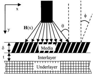
Fig. 1. System geometry with tilted media.
This paper examines these issues in detail to determine whether media can be designed to fulfill these conflicting requirements. We adopt the stricter SNR requirement of [2] and assume 6-nm grains. We also assume that although the attainable write head field will exceed that from an isolated single pole, it will not be possible to fully achieve 2.4 T. In a recent paper, Kanai et
al. suggest that a write field of 1.8 T (18 kOe) can be achieved
for a 1 Tb/in head meeting reasonable design criteria [3]. We have assumed a peak write head field of 1.75 T (17.5 kOe).
II. SEMIANALYTICALMODEL
A. Noninteracting Grains
For generality, we assume a geometry as shown in Fig. 1. The medium may or may not be “tilted” [4]. It is assumed that there is an underlayer. The write head may have any geometry and is shown here as a single pole only for simplicity.
Each grain of the medium is assumed to have a single anisotropy axis tilted at an angle to the film perpendicular so that the head field makes an angle to the perpendic-ular and to the easy axis of the grain. This angle is critical in determining the switching behavior of the medium [2], [5], and we therefore provide a full analysis. The easy-axis tilt may arise from physical tilt of the columns or tilt of the crystalline orientation of the grains, but if the columns are physically tilted, the crystalline axes are assumed to be tilted at the same angle as the physical tilt. The grains individually are assumed to be below the critical size for single domain behavior. The possibility of grains reversing magnetization by curling has been neglected and grains are assumed to switch at a field given by the Stoner–Wohlfarth switching astroid
(1)
Fig. 2. Defining the angles of the applied field and the anisotropy axis.
where is the anisotropy field, and
(2)
It is assumed that the anisotropy field and tilt are distributed with normalized probability density functions and , respectively, and that the anisotropy axis lies in the – plane. The probability density function can be determined by inverting (2) to obtain , and using
(3)
in which it must be recognized that the astroid function is multivalued.
The switching field distribution can now be obtained from (1) and (3) as
(4)
The coercivity of a noninteracting system can be found by solving
(5)
or for a symmetric distribution directly from and (2)
(6)
The magnetization is assumed to always be aligned along the anisotropy direction. In this case, the susceptibility is most use-fully defined as
(7)
where is the magnetization parallel to the anisotropy di-rection, is the magnitude of the field applied in the direction , and the prime indicates that interactions have been ignored. Neglecting reversible magnetization changes, the susceptibility can be obtained from the switching field distribution
(8)
[image:3.612.305.552.61.149.2]Equations (4), (6), and (8) describe the desheared loop for perpendicular media in which the anisotropy is confined to
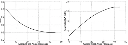
Fig. 3. Angular variation of coercivity (left) and susceptibility (right) for a noninteracting assembly of perpendicularly oriented particles.
[image:3.612.100.226.62.174.2]Fig. 4. Effect of dispersion upon coercivity.
Fig. 5. Effect of dispersion upon susceptibility.
the – plane. In practical media, dispersion will spread the anisotropy axes into three dimensions as shown in Fig. 2.
In the three-dimensional (3-D) case
(9)
and the probability density function for can be obtained from
(10)
From (9)
(11)
Typically, is a normal distribution and is uniformly dis-tributed between 0 and 2 , so that and
(12)
after which the hysteresis loop can be obtained by appropriate substitution for in (3) to (8). and are shown in Fig. 3 for a perpendicularly oriented medium with ,
%, %, % %.
[image:3.612.303.552.305.399.2]is significantly reduced by dispersion in . Dispersion in has little effect upon the coercivity and susceptibility at 45 , be-cause at that applied field angle the switching field is relatively insensitive to angle. For field angles nearer to 0, coercivity and susceptibility are reduced by dispersion in . At low angles, the susceptibility of a two-dimensional (2-D) assembly is signifi-cantly different from that for the 3-D assembly and is shown in Section III-B1. This shows that the 3-D calculation is necessary in order to predict performance.
Where the easy axis of a grain and the applied field are not perfectly aligned with the perpendicular direction, the hysteresis loop of the grain will not be perfectly square and the magne-tization change upon switching will be reduced by reversible rotation of the magnetization. For small easy axis and field an-gles, the magnetization angles are small and the perpendicular component of magnetization (being proportional to the cosine of the polar angle) remains close to . The effect of reversible magnetization changes upon the susceptibility of an assembly of noninteracting grains is determined in Section III and is shown to be 5% for the values of dispersion used in this paper.
Although this analysis neglects demagnetizing fields and interactions, it is nonetheless useful. At the coercive point the average demagnetizing and exchange fields are zero, so the coercivity predicted by (6) is a reasonably accurate estimate. The susceptibility predicted is that of the array of grains with all interactions removed, which is necessary for slope theories of recording. This is not necessarily the same as the slope of the desheared loop as deshearing will not in general remove the effect of exchange interactions. As shown in Fig. 3, changing the applied field angle from 0 to 15 approximately doubles the susceptibility and decreases coercivity by 25%. In order to make a correct prediction of performance, vector calculations must be performed, and calculation of the interaction fields is necessary.
B. Interactions and Demagnetizing Fields
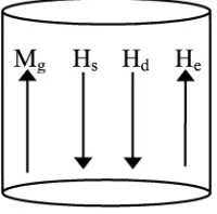
A single grain within a perpendicularly oriented medium magnetized to saturation experiences interaction fields as shown in Fig. 6.
1) Self-Demagnetizing Field : The self-demagnetizing
field arises from the magnetization of the grain itself, varying in direction as the grain magnetization rotates, and therefore cannot be considered as an external field.
We assume that
(13)
i.e., that the demagnetizing factors , , and are positive and that all off-diagonal terms of the demagnetization tensor are zero. For a perpendicular cylindrical grain with no underlayer,
and (SI units). The volume
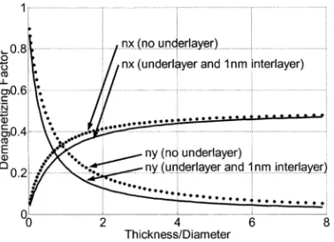
[image:4.612.379.479.65.164.2]av-eraged or magnetometric self-demagnetizing factors of cylin-ders have been calculated by Chen et al. [6]. The presence of a soft underlayer (SUL) significantly modifies the demagnetizing factors, and removes the constraint , as the field is averaged only over the volume of the actual grain, while the field originates from the total volume of the grain and the
Fig. 6. Single grain in a perpendicular medium magnetized to saturation.
image. To compute values of demagnetizing factors, the grain was assumed to be perfectly imaged in the underlayer and the grain volume averaged field due to the integrated surface charge on the grain and image was computed numerically with results shown in Fig. 7.
The self-demagnetizing field gives rise to a shape anisotropy
(14)
If the medium is tilted, then the appropriate coordinate trans-forms must be made to obtain the demagnetizing factors along and across the grain axis.
2) Demagnetizing Field : The perpendicular
demagne-tizing factor for a thin film is with or without an underlayer. For a sparsely populated film the volume aver-aged demagnetizing field experienced by a grain due to the other grains in the film may be reduced [7], but in a densely packed film the perpendicular demagnetizing factor will be close to 1.0. Since the demagnetizing factor of a thin film incorporates the whole of the film material, it includes , and so for a saturated film
(15)
where is the volume averaged magnetization of the film, and is the grain packing fraction.
3) Exchange Field : Each grain experiences an exchange
field due to neighbor grains. The strength of the exchange field depends upon the intergranular exchange constant and the ge-ometry of the grains. For a saturated perpendicularly magne-tized film, the average exchange field can be written
(16)
where is the exchange constant for the material in the grain boundary, incorporates all geometric factors (surface contact area, separation, etc.), and is the ratio of the exchange field to the magnetization in a saturated film. The exchange field and the origin of (16) are discussed later in this paper (44)–(50). In this paper, we assume that is constant, i.e., that the ratio of ex-change field to demagnetizing field is fixed. It is implicit in that assumption that changes to would require corresponding changes in or .
4) Simple Hysteresis Loop Shear Model: The interaction
fields (15) and (16) can be summed to obtain the total interac-tion field for a saturated film. If we assume that the interacinterac-tion field is proportional to , then
Fig. 7. Demagnetizing factors for columnar grains with and without underlayers.
The total field experienced by a grain is
so that the susceptibility can be found from (8) and (17) as
(18)
C. Media Constraints for Perpendicular Recording
A usable medium for perpendicular recording must satisfy three basic constraints: it must have low enough anisotropy that the write head can saturate the medium, it must have high enough anisotropy to remain thermally stable for ten years, and it must support narrow transitions. In order to evaluate these constraints, it is necessary to determine the peak demagnetizing fields for recorded data.
1) Demagnetizing Fields: During recording the medium is
not uniformly saturated, and thus the demagnetizing field is lower than . A simple model was constructed to estimate the demagnetizing fields for a wide range of different configu-rations, an example result being shown in Fig. 8.
The following parameters were assumed: track pitch 63.5 nm, track width 50 nm, bit spacing 10 nm, write pole width 50 nm, write pole length 200 nm, interlayer thickness 1 nm, and medium thickness 20 nm. Magnetization was taken to be either or only, and assigned in the tracks according to a pseudorandom sequence. The demagnetizing field was calculated by assuming surface charge of on the top surface, and on the bottom surface. Both charges were imaged in the underlayer and the total demagnetizing field calculated according to
using a fast Fourier transform (FFT) method. The area of the region was chosen to be large enough that for a uniform dc magnetization, the demagnetizing field was 0.95 , i.e., a 5% error. This area accommodated 11 tracks each of 70 bits. During recording, the region under the pole is magnetized in the same sense as the bit being recorded as shown in Fig. 8. Pseu-dorandom data were generated for all 70 bits of all 11 tracks on an initially dc magnetized sample, and the resulting
demag-Fig. 8. Magnetization pattern (left) and demagnetizing field (right) shown during recording of the center track.
netizing field within the region of the bit being recorded was (mean standard deviation for 100 dif-ferent configurations). With samples that were initially ac de-magnetized (randomly by pixel), the demagnetizing field was . The difference between dc and ac demag-netized initial configurations is due to the material between the tracks. In a real system, this would probably be magnetized with noisy signal during recording so that dc magnetization is prob-ably pessimistic. Recalculation without the large dc area under the pole gave very similar results for pseudorandom data across all tracks. For isolated tracks (center track only) in an ac-erased medium the demagnetizing field was very similar to multiple tracks, at , but for a dc-erased medium the field for one isolated track is higher, at . As expected, writing onto dc-erased media is harder when writing in the same sense as the original magnetization direction. If we assume that perpendicular media will not be uniformly dc mag-netized prior to recording, the largest demagnetizing field ex-perienced will be 0.70 (mean 3 standard deviation).
We have employed , which is a
more conservative assumption than made by Honda et al. [8]. It should be recognized that servo sectors may have lower fre-quency regions than occur in the pseudorandom data used here, and thermal stability for servo may require stricter criteria or to be designed to tolerate higher thermal decay rates than data.
2) Saturation: During recording, it is necessary for the head
to be able to saturate the medium. This can be expressed as a re-quirement that the head field must be large enough to magnetize the last grain to reverse. In this state, the medium is uniformly magnetized except for the grain of interest. Assuming a linear hysteresis loop of slope , the field required is . The coercivity can be expressed as , where in-corporates the angular variation of switching fields as described by (3)–(12). Then
(19)
and if the head field is limited to , then
(20)
[image:5.612.71.260.62.199.2]takes no account of head field angle. We assume that at satura-tion the magnetizasatura-tion is aligned with the applied field, when , and the demagnetizing field in a uni-formly saturated film can be obtained by modification of (17)
(21)
where and are calculated taking account of the tilt of the column. The procedure to determine a maximum value for is as follows.
a) For a given head field , calculate . b) Using and the tilt , calculate . c) Using (21) calculate the interaction field
for the saturated medium, taking . d) Calculate the magnitude of the total field
.
e) Calculate the maximum of . f)
(22)
This process [a)–f)] must be repeated for each value of .
3) Thermal Stability: We require that no more than 10% of
grains reverse due to thermal activation in a ten-year period. Assuming that grains smaller than the tenth percentile grain by volume will thermally reverse, while those larger will be stable, a simple expression can be obtained by considering the com-ponent only, in which case
(23)
where is the volume of the tenth percentile grain, and the internal field can be obtained from the linear – loop model
as so that
(24)
and thus
(25)
For a given value of , must be lower than the value implied by (25) to ensure thermal stability.
Where the medium is tilted or there is an off-axis external field (such as during off-track erasure), a dc-saturated film ex-periences an internal field of
(26)
where can be calculated from (21). For a field of magnitude at an angle
to the easy axis the energy barrier for the tenth percentile grain can be obtained from the Pfeiffer approximation [9] to be
(27)
where is given by (1) and (2) and
so that the thermal stability criterion can be expressed as
(28)
or
(29)
which gives the relationship between and for thermal stability.
4) Transition Width: It is natural to calculate an “ ”
param-eter from a slope theory. However, the large variations of co-ercivity and susceptibility with field angle must be taken into account, as the head field varies in magnitude and direction as a function of position. Vector slope models were developed for metal evaporated tape [10]–[12]. We simplify the problem by assuming that in the absence of “tilt” the magnetization is con-fined to the perpendicular direction, that
(30)
and that the hysteresis loop can be described by
(31)
where is as defined by (7) and , the total field, is the sum of external and internal or interaction fields. At the transition center , so that the location of the transition center ( ) can be found as the point at
which , where is the angle of the
head field. To obtain the slope at the transition center
At , and so
(32)
The final term of this expression was given by Gao and Bertram [13] and a similar approach is used to model the temperature gradient in HAMR systems [14]. It is necessary to include the exchange field here because was defined earlier as the susceptibility of the array of grains with all interactions removed. is therefore not necessarily the same as the slope of the desheared loop. Standard expressions for demagnetizing fields [15] can be readily modified to account for an underlayer (we have ignored the interlayer for simplicity, though it could easily be included at the cost of additional terms)
The exchange field being local can be taken as , so that
(34)
It must be noted that the field in (32) is defined parallel to . Since we have assumed zero tilt, , , and are in the perpendicular direction. Thus, a small increase in ,
, is in the perpendicular direction and the increase of [which is in the direction ] is
(35)
from which “ ” can be found by solving
(36)
where
An alternative method of evaluating the “ ” parameter is to determine the location of the nucleation and saturation head fields. At each of these points, the medium is saturated (in one direction or the other) and the internal field can be calculated from (21) taking . To obtain the location at which the head field will just nucleate reversal, we calculate the total field as (the interaction field enhancing the head field at the nucleation point). We then identify the location at which , where is the angle of the total field. The location at which the head field just saturates can be similarly identified from a total field in which the interaction field opposes the head field. The separation of these two loca-tions is the total width of the transition, i.e., . This method does not allow for a finite intrinsic switching field distribution but does allow for asymmetry in the transition, as discussed by Nakamura [16]. In practice, the demagnetizing field at the satu-ration and nucleation points may be lower than this assumes, for example, on thicker media or where track widths are narrow or at the nucleation point in high-frequency data (which is farthest away from the saturated region under the pole and, therefore, does not experience the field from a long saturated length of track). This method may therefore tend to overestimate transi-tion width.
5) Limit of Intergranular Exchange: Exchange coupling
be-tween grains acts to maintain the magnetization of a uniformly magnetized region, and thus acts to enhance thermal stability of dc regions or long wavelength sections of a data pattern. Ex-change coupling also acts in the same sense as the head field gradient and in opposition to the demagnetizing field gradient during writing of transitions, and should therefore act to re-duce written transition width and the width of the track edge. However, exchange acts to align magnetization and makes small
Fig. 9. Two neighboring grains in a saturated perpendicular medium (left) and after one grain has thermally reversed (right). The fields shown are those experienced by the neighbor (right-hand grain) due to the switching grain (left-hand grain).
domains energetically unfavorable, so that excessive exchange coupling could act to assist thermal decay of high frequency information. We consider two neighboring grains, and imagine that one of the grains reverses due to thermal excitation.
When the left-hand grain of Fig. 9 reverses, the internal field in the direction opposite to in the right-hand grain increases by an amount , so to ensure that the reversal of one grain does not destabilize neighbors and cause domain growth it is necessary to ensure that . From (16), the ex-change field arising from one of nearest (touching) neigh-bors can be expressed as
(37)
and the demagnetizing field due to one neighbor is
(38)
where is the interaction factor for neighboring grains. Thus, to ensure that thermally demagnetizing grains do not destabilize their neighbors
(39)
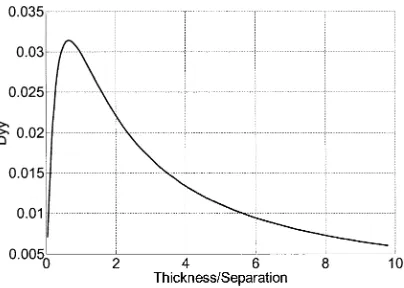
The interaction factor must be calculated numerically via the neighbor grain volume averaged field arising from the integrated surface charge on the source grain and its image in the underlayer, in the same manner as for the self-demagnetizing factors of Fig. 7. An example is shown in Fig. 10 for neighboring cylindrical grains, which was computed assuming an interlayer thickness nm and a 0.5-nm grain boundary within a 6-nm grain diameter. Medium thickness was varied between 0.25 and 50 nm.
For nm and diameter nm, .
As-suming hexagonal packing, and . Thus, for the geometry assumed for Tb/in media, the exchange field
.
D. Results—Analytical Model
Fig. 10. The neighbor magnetostatic interaction factor as a function of medium thickness for a perpendicular medium with a soft magnetic underlayer.
Fig. 11. Constraint functions for 6-nm grains.
to match these potentials and their normal gradients along their common boundary. Fourier transforms ensure that the potentials also match up on the surface of the pole. It is only necessary to solve for the potential at the air-bearing surface (ABS). Having done this, we use potential theory to determine the potential at any level between the ABS and the SUL. This stage corrects for the initial approximations used to describe the potential between the faces of the pole or shields and the SUL. The magnetic field components used in the recording simulation are then calculated with the help of an FFT algorithm. Although the assumption of equipotential surfaces is a simplification for a very small pole, this model does provide realistic approximations to head fields without resort to full FEM analysis.
The geometry of the head used was: pole width 50 nm, pole length 200 nm, pole to side shield spacing 12.5 nm, and pole to end shield spacing 50 nm. A peak field of 17.5 kOe was assumed. Media parameters assumed were interlayer thickness 1 nm, medium thickness 20 nm, , %,
%, %, grain boundary thickness
0.5 nm, packing density 80%, standard deviation of grain cross sectional area 30% of mean area, .
The vector versions of the writability criterion (22) and the thermal stability criterion (29) were evaluated for a range of values for various mean grain diameters. It was found that a mean diameter of 6 nm was required to allow both criteria to be satisfied, for which a graph is shown in Fig. 11.
The viable region for a recording medium is the region bounded below by the thermal stability criterion and above by the writability criterion. For these medium parameters and head field, the slope theory (36) gives an “ ” value that does not vary substantially within the viable region and that is of order 1 nm. Calculation of “ ” from the location of the nucleation and saturation fields gives an “ ” value that increases from 3 nm in the lower left corner of the viable region to 6 nm in the upper right corner. These values agree with the results of Mallary et al. [2], who predicted “ ” parameters of 0.2 to 0.5 times the grain diameter for a shielded head. For very high field gradients, it is likely that the transition shape during writing is not well approximated by the arctangent profile assumed by (36). We have selected the lower left corner of the viable region as optimal for ultrahigh-density storage, giving mA and A/m. This value of includes the shape anisotropy of the grains. The intrinsic (crystalline) anisotropy of
the material is A/m or J/m .
For these media values, the head field gradient at the write point is 563 Oe/nm.
III. MICROMAGNETICMODEL
A. Model Description
Predictions of the micromagnetic model have been published previously [5], [19]–[22] with partial model descriptions. A complete description has not yet been provided. The model assumes that magnetization is uniform within a grain, and that there is a wall or discontinuity within the grain boundary. This is consistent with assuming weakened exchange within the grain boundary and grains small enough that there can be no nonuniform magnetization or incoherent reversal modes within grains. A fully arbitrary grain geometry is assumed, and accurate calculation of grain–grain magnetostatic and exchange fields is included. For dynamic calculations, we employ a Krylov solver [23] to solve the Landau–Lifshitz–Gilbert (LLG) equation, which we express in polar coordinates to reduce the number of equations and to avoid the need for renormalization to maintain constant
where and are the magnetization polar and azimuthal angles, respectively, and the subscript indicates that we are using the Gilbert form. For or , the azimuthal term becomes in-finite, and some authors (e.g., [24]) have employed coordinate transforms to avoid this problem. We note that this is only a nu-merical problem as the accuracy of the azimuth is unimportant
for or , so we set in the
Fig. 12. Cross section of grains used for the micromagnetic simulations.
the and . Although we limit to prevent it from becoming infinite, it can still become large as becomes close to 0 or . In such a region, the ODE solver will employ time steps sufficiently small to accurately compute , which is unnecessary for these values and will significantly degrade performance. Sensible selection of axis orientation will mini-mize this. The local field experienced by each grain is the sum of external, crystalline anisotropy, magnetostatic, and exchange fields. Grain shape anisotropy is implicitly included in the mag-netostatic field calculation as the self-interaction field.
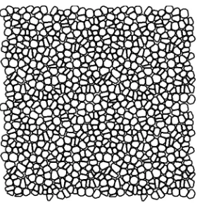
1) Grain Geometry: The model is designed to accommodate
fully arbitrary grain shapes and positions by employing a hier-archical method to compute the demagnetizing fields [21]. The cross section of grains used in this work is shown in Fig. 12.
This grain distribution has a mean grain area of 6 nm 6 nm, including a 0.5-nm grain boundary, with an approximately lognormal distribution of grain areas with (area)/area 0.32. To generate the grains, we take a hexagonal or cubic lattice of points and randomly displace each point in two dimensions. By varying the range of the random variables used, we can control the ultimate randomness of the structure. We then perform a Voronoi construction and generate Voronoi polygons. The Voronoi polygons are then shrunk to allow a grain boundary of the required thickness between each surface. Within each Voronoi polygon, we then nucleate an -sided polygon of zero radius at the center of mass. This polygon is then inflated gradually. If any point on the polygon hits the boundary of the Voronoi polygon, its position is frozen. This process continues until the grain occupies a specified fraction of the area of the Voronoi polygon. Using this technique, we can generate grains with independently specified (area)/area, grain boundary thickness, and packing fraction. If required, the system can be stretched in one dimension at the first stage to simulate grain shape distortion due to surface texture or tilted deposition. The initial stage of the process employs a regular lattice and, therefore, the associated indexing information is still available. This means that such pseudoirregular structures can be incorporated into FFT algorithms in the manner described by Jones et al. [22]. In this work, we employ a hierarchical model that makes no assumptions of order.
2) Magnetostatic Field Calculation: To compute the
de-magnetizing fields the method described in [21] is slightly extended, in that we accurately compute the magnetostatic
fields due to near neighbors. In the simulations presented here, for neighbors nearer than 30 nm (6 mean diameter, 1.5 thickness), the magnetostatic interaction fields are computed by
(40)
where the 3 3 interaction matrix is precalculated by inte-gration over the surface of grain (the source) and the volume of grain , for example
(41)
Equation (41) is readily computed numerically taking full ac-count of shape since the vertical (outer column) surface of the source grain is built of rectangular charge sheets defined by the grain polygon, and the top and bottom faces can be approx-imated by subdivision into rectangular sheets (typically ). In the case of perpendicular media where there is an SUL, each grain generates an image whose magnetization is related to that of the grain by
(42)
so that the total field experienced by a grain can be computed as
(43)
where is the field experienced by grain due to the image of grain . Using this formulation, additional computa-tion is confined to the precalculacomputa-tion of image interaccomputa-tion factors , and the simulation time is not increased. The method could readily be extended to include imaging in the head, except that an infinite series of images would be generated that would have to be truncated at the point that achieved acceptable accuracy.
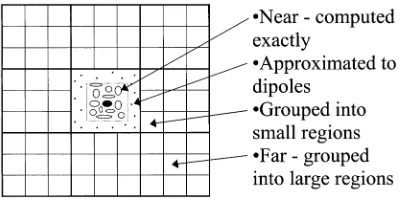
In the hierarchical model, we employ a simple dipole expansion in which increasingly large regions of material are approximated to single dipoles as distance from the field calculation point increases, as shown in Fig. 13. The total field is computed as a sum of exact grain–grain calculations, simple dipole grain–grain calculations, and dipole calculations in-volving medium and large-scale regions of material. Neighbor lists are required for all interactions except for the largest scale regions. For those large regions within which higher resolution calculations are performed the interaction matrices are initially set to zero. Periodic boundary conditions are applied and accuracy criteria are used to determine the boundaries between different approximation regimes.
Fig. 13. How the field at the shaded grain is computed using increasing approximation as range increases.
this paper) which tile to fill space. The interaction matrices for this basic set of grains are then all that need to be calculated and stored.
Periodic boundary conditions are applied so that in the field calculation, the large region containing the target grain is at the center of the material that contributes to its magnetostatic field as depicted in Fig. 13. Nevertheless, the magnetostatic field cal-culation is effectively truncated at a range half the sample size from the target grain as described by Nakatani et al. [24]. For in-plane materials this effect is rarely a problem, as the field error is simply that due to a charge sheet the thickness of the material around the circumference. For perpendicular media the error is more significant—in the worst case of a dc-magnetized sample, the missing field is that due to two infinite charge sheets on the top and bottom surfaces of the material with holes corre-sponding to the region for which we have actually computed the field. This can yield a significant error and must be corrected. We correct this by repeating the sample periodically to fill space, assuming that the magnetization distribution is the same in all repeats and truncating the series at a reasonable range. Thus, the field experienced by grain is
where the sample is repeated times and is the interac-tion matrix for the th repeat. The field due to the sample itself is computed hierarchically as described above. For the repeats, it is assumed that the range is sufficient that only large regions need to be employed; thus, the summation can be performed within the interaction matrices for the large regions during the precomputation stage and without any additional computational cost during simulation.
FFT calculations provide an efficient method of computing the sum of grain–grain magnetostatic interactions in a system of identical grains on a regular lattice with periodic boundary conditions. A similar correction is therefore required for FFT methods when simulating perpendicular media.
3) Exchange Interaction: We assume that exchange
interac-tion is weakened in the grain boundaries and that magnetizainterac-tion is uniform within the grains, so that exchange energy arises only from magnetization changes within the boundary and takes the form
(44)
where is the exchange constant for the intergrain material and is the separation of the grain surfaces. Assuming a constant
spacing between grains and that varies linearly across the intergrain boundary, the total energy is
(45)
where is the film thickness and is the in-plane length of the boundary. For arbitrary shape grains will generally not be constant and (45) should be written
(46)
where is the in-plane direction along the grain boundary. The exchange field is then given by
(47)
where is the volume of grain . Thus
(48)
It is worth noting that the classical approximation of (44) assumes a small angle and that for large magnetization differ-ences, such as might be expected in perpendicular media, the approximation is not good. Taking the first form of exchange energy would result in a field of the form
(49)
where . Equation (48) or (49) yield similar torque, and so either could be used in dynamic calculations. In thermal stability calculations, the effect is significantly dif-ferent. In a saturated film (48) yields a field parallel to that reinforces magnetization, while (49) yields zero field. We there-fore use (48). In [20], dynamic calculations were performed using a form similar to (49), except that the energy of the wall was shared between the two grains and . That formulation yields identical results to (49) provided that is doubled. Since the value of the intergrain exchange constant is unknown, its value is usually set to obtain a required ; consequently, this error did not significantly affect the results or conclusions presented in [20].
The average over the whole film of the perpendicular compo-nent of the exchange field can be determined from (48)
(50)
where is the average perpendicular component of magneti-zation and embodies all geometric terms.
4) Thermal Activation Model: For long-term thermal decay
studies, we use a probabilistic model. The local field is com-puted at each grain using the methods of Sections II and III above excluding both crystalline and shape anisotropy fields. The shape anisotropy is approximated from the self-magneto-static interaction matrix by assuming a cylindrical shape
We then employ an iterative technique in which we step time in equal increments of (time). During each time step, we cal-culate the energy barriers for reversal in both directions for each grain, and thus the probability of reversal during that time step. Each grain is switched (or not) according to a master equation approach [25] as described in [26] and [27].
5) Dynamic Calculations: In simulations where uniform
ternal fields (e.g., hysteresis loops) are applied, the required ex-ternal field is specified in polar coordinates at discrete times. The Krylov ODE solver solves the LLG and determines time steps according to its own accuracy criterion. The external field is determined at each time step by timewise linear interpola-tion in polar coordinates between the field values at the speci-fied times. Consequently, there are no explicit field steps and the field varies as smoothly as necessary for the ODE solver. This allows arbitrary rotating and linear field sequences to be applied with no numerical artifacts.
For recording simulations, we use output from FEM models or equipotential models to define a 3-D head field throughout the 3-D space between the head and underlayer. Where an FEM is used to predict head fields, these can be generated at var-ious write currents to characterize saturation. The required write current is specified at arbitrary (but significant) times (e.g., for each, bit the start of the current rise, the end of the current rise, and the end of the bit cell). The ODE solver then solves the LLG from the start time through to the end time of the entire simulation in one call to the solver routine. At each time step of the solver, the write current is determined by interpolation between the user-specified current/time points to determine the write current . The head field is then determined by inter-polating between FEM outputs at different currents to provide a head field on a uniform grid at the given time. The field at each grain is then determined by spatial interpolation between the regular grid points. The location of the head (and, thus, the origin of the head field) is determined from the time and the velocity.
For long recording simulations, such a simple method would require excessive memory and simulation time, as large regions of material would be subject to zero field for large parts of the simulation. We minimize computation time and memory by defining an “active” region of the simulation that extends slightly beyond the region in which the head field is nonzero (see Fig. 14).
By numbering the grains transversely (cross track) in medium-sized elements of the hierarchical calculation, the active region can be stepped in units of the medium cell size rather than in tiles, allowing the active region to be only slightly larger than the area over which the head field is defined. The magnetization evolves only in the active region and therefore the magnetostatic field need only be computed there, but the calculation of the magnetostatic field incorporates all of the grains in the system as sources.
B. Results—Micromagnetic Model
1) Susceptibility Calculations—No Interactions: Hysteresis
[image:11.612.333.521.60.153.2]loops were calculated without magnetostatic or exchange inter-actions for 19 600 grains of a perpendicularly oriented medium ( ) with , distributed uniformly over 0–2 ,
Fig. 14. How the system is composed of tiles of the basic grain structure, only a selection of which are active at any given time. As the head moves along the total region of the simulation, the “active” region moves to always contain it.
Fig. 15. Coercivity (left) and susceptibility (right) calculated by (6) and (8) (solid lines) and micromagnetic model (circles). Easy axes distributed in three dimensions.
%, %, %.
Coer-civity and susceptibility (defined as ) were calculated for fields applied at a range of angles to the perpendicular direc-tion. For the susceptibility calculations, a hysteresis loop time period of 40 ns (25 MHz) was used to avoid any high-frequency precessional effects. The damping constant was chosen to be 0.05 for all calculations presented in this paper. The micro-magnetic model shows excellent agreement with the analytical model, with differences lower than 2.5% over the whole angle range (see Fig. 15). For small angles, the response time of the grains to perpendicular fields is very long, and so a dynamic calculation must be performed with a slowly varying field. The coercivity values in Fig. 15 were calculated with field reversal times of 200 ns. This behavior is consistent with that observed experimentally by Coffey et al. [28], which lends support to the assumption that the grains reverse as uniformly magnetized Stoner–Wohlfarth particles at low frequencies.
If is set to zero, then the easy axes are confined to the – plane (2-D) and the results change as seen in Fig. 16.
For 2-D distributed easy axes, the agreement is also excellent up to 20 and better than 5% over the whole range. The analyt-ical and micromagnetic models both show a significant differ-ence in the susceptibilities predicted by 2-D and 3-D oriented assemblies of grains, demonstrating that only a full calculation can correctly describe perpendicular media.
2) Uniform Field Simulations of Tb/in Media: In
Sec-tion II, we determined an optimal medium design for 1 Tb/in based upon thermal stability and writability. The parameters
selected were mA, J/m (crystalline
anisotropy), and , which gives
for a dc magnetized sample. Other parameters were interlayer thickness 1 nm, medium thickness nm, , distributed uniformly over 0–2 , %, %,
[image:11.612.304.552.206.294.2]Fig. 16. Coercivity (left) and susceptibility (right) calculated by (6) and (8) (solid lines) and micromagnetic model (circles). Easy axes distributed in two dimensions.
Fig. 17. The hysteresis loops for uniform applied fields at angles 0 , 5 , 10 , 15 ; . . . ; 45 to the perpendicular. The vertical bold lines show 17.5 kOe (peak head field) and 14.2 kOe (field at which the medium is expected to saturate with the field angle at 30 ).
packing density 80%, and standard deviation of grain cross sectional area 30% of mean area.
For the head field used (described in Section II-D), the op-timal location on the head field contour is where the field angle is 29 and the magnitude is 1.13 MA/m (14.2 kOe). The defi-nition of saturation assumed is that the last grain has switched from positive to negative magnetization. Fig. 17 shows the per-centage of grains with positive as a function of applied field for fields at 5 intervals. The hysteresis loop period was 20 ns (50 MHz).
Fig. 17 shows that the saturation field is a strong function of angle as expected, and as shown in [5]. With the field applied at an angle of 30 , the medium does not quite saturate at field magnitude 14.2 kOe as might be expected. This is because the analytical model only aims for saturation during writing, when the medium is not uniformly magnetized and can be assumed. In Fig. 17, the field is uniform over the whole sample and at saturation the sample is uniformly magnetized, with the result that saturation is more difficult than during recording. This result suggests that the medium will meet the design target at low frequencies. At higher frequencies, the coercivity and saturation field will rise as a result of precessional switching effects. This effect is not included in our analytical model, and some allowance may need to be made at very high record frequencies. High-frequency reversal in perpendicular media is discussed in [20].
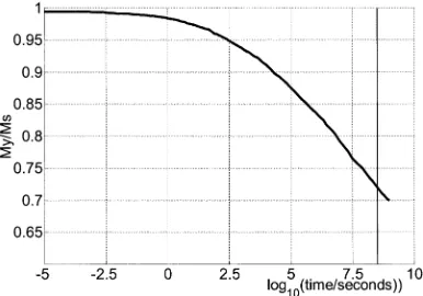
[image:12.612.71.260.199.338.2]A uniformly magnetized (saturated) sample was simulated in zero field and allowed to thermally decay for 10 s. The design criterion of 10% of grains thermally decaying in ten years would result in a final magnetization of 0.8 . The higher decay rate
Fig. 18. Thermal decay of a uniformly magnetized sample in zero field. The bold vertical line represents ten years.
Fig. 19. Top: a 10-nm bit spacing track (1 Tb/in ) written between prewritten 11- and 12-nm bit spacing tracks, immediately after writing. Bottom: a 10-nm bit spacing track (1 Tb/in ) with 15- and 20-nm tracks postwritten either side, after ten years thermal decay in zero field. The horizontal lines show the edges of the read track.
shown in Fig. 18 results from the uniform magnetization, which generates a larger demagnetizing field than would be expected during recording ( instead of ), and drives a higher rate of decay.
3) Recording Simulations: The head described in
Sec-tion II-D was employed in recording simulaSec-tions. A head/medium velocity of 6.35 m/s was employed, corre-sponding approximately to an outer track of a 1-in-diameter disk at 5400 r/min. A head field rise time of 0.5 ns was assumed. The track pitch was taken to be 63.5 nm, write width 50 nm, and read width 35 nm. At this track pitch, a 10-nm bit spacing (2540 kfci) corresponds to 1 Tb/in .
Fig. 20. The decay of mean peak height with linear density for the three initial configurations: dc magnetized (asterisks), ac demagnetized (triangles), and with two adjacent tracks written (circles).
Fig. 21. Standard deviation of the peak height/Ms as a function of linear density for the three initial configurations—symbols as Fig. 20.
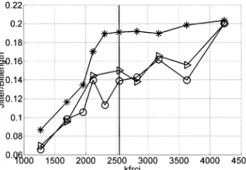
Fig. 22. Jitter/bit length as a function of linear density for the three initial configurations—symbols as Fig. 20.
[image:13.612.340.514.231.352.2]decayed at 50 C for ten years. These simulations show that recording at 1 Tb/in is possible. At 2540 kfci, the magnetiza-tion remains above 0.95 after ten years. is 10%, jitter is 15% of the bit length. The fitted “ ” parameter at 1 Tb/in is 2 nm, which is midway between the 1 nm pre-dicted by the slope theory and 3 nm prepre-dicted by the nucleation and saturation points. Slope theory predicts an “ ” value below the grain size limit of nm and the fitted values of “ ” shown in Fig. 24 for all configurations are 2 nm. It is there-fore likely that “ ” is limited by grain size in this case. Other (unpublished) simulations of lower coercivity media have pro-duced results in agreement with the slope theory. When writing a track on a uniformly dc-magnetized medium with no adja-cent tracks, the demagnetizing field of the surrounding material makes it easier to write bits in the opposite sense of the dc mag-netization than in the same sense. The existence of “easy” and
Fig. 23. Mean magnetization as a function of linear density for the three initial configurations—symbols as Fig. 20.
Fig. 24. The “a” parameter as a function of linear density for the three initial configurations—symbols as Fig. 20.
“hard” magnetization directions means that bits written in the opposite sense to the surrounding dc magnetization tend to be larger than those written in the same sense, giving a net dc bias to the signal as shown in Fig. 23. The resultant bit-size varia-tion gives rise to jitter as shown in Fig. 22. Although it is highly unlikely that disks will be uniformly dc magnetized, such an ef-fect will occur to a lesser extent when HF data follows LF data, or when long dc sections appear in adjacent tracks, or in servo sectors.
The effect of thermal decay is small, with no noticeable effect on jitter or peak height variance. There is a small increase in “ ” parameter as shown in Fig. 25, which results in a small decay in magnetization at high frequencies as shown in Fig. 26. This is consistent with the suggestion that exchange coupling will lead to degradation of high frequencies only, and that the design parameters chosen are acceptable for 1 Tb/in .
We have not studied thermal decay at lower frequencies in de-tail, but it may be anticipated that for very low frequencies the demagnetizing field will be higher and thermal stability may be compromised. There is some evidence of this in the lower image of Fig. 19, in which the imprint of the write pole shows a number of reversed grains. Although the lower value of exchange se-lected has ensured that these have not propagated and grown, it is clear that large dc areas are not fully stable, and it is necessary to evaluate performance for higher values of exchange.
4) Higher Exchange Coupling: If the ratio is increased, higher stability of dc is expected, and this is con-firmed by Fig. 27.
[image:13.612.72.255.237.360.2] [image:13.612.75.252.401.523.2]Fig. 25. “a” parameter immediately after writing (stars) and after ten years decay at 50 C (circles).
Fig. 26. Mean peak height immediately after writing (stars) and after ten years decay at 50 C (circles).
Fig. 27. Micromagnetic model predictions of the thermal decay ofhM i in an initially dc saturated sample for different values ofC = He=Hd.
of the energy barrier against reversal from the initial (“up”) di-rection to the opposite didi-rection (“down”). For most grains, as the average magnetization of the sample thermally decays, the energy barrier rises, since the demagnetizing field is reduced. However, for neighbors of grains that have reversed, the energy barrier falls as shown in Fig. 28. A similar study for
(the value used for Tb/in simulations) presented in Fig. 29 shows minimal barrier reduction.
[image:14.612.338.519.216.341.2]It is expected that the postulated thermal decay mechanism of destabilization of neighbor grains will act to produce domain growth and mitigate against high frequencies for values that are too high. This effect can be seen by study of ac-erased sam-ples. An ac-erased state is generated by raising the temperature to 10 K and running the long-term thermal decay process for 1 s, which totally randomizes the system. The dynamic solver is
Fig. 28. Scatter graph of energy barrier after ten years thermal decay versus initial energy barrier for a sample with 4900 grains andC = 0:3 (left). The diagonal line shows equality. The plot on the right shows only those grains whose magnetization has reversed, which shows that grains withEb < 42K T decay as expected.
Fig. 29. Scatter graph for a sample withC = 0:1.
then run for 10 ns to allow the system to reach dynamic equilib-rium. Then, the thermal solver is run again for ten years at 50 C. Qualitative observation of the images shown in Fig. 30 suggests that for there is minimal domain growth, while for there is significant domain growth that would influ-ence the ability of the medium to retain high-frequency data over long periods.
Recording simulations at confirm that high-fre-quency performance is reduced with reduced peak magnetiza-tion and increased noise as shown in Figs. 31 and 32. The “ ” parameter of 2 nm is not significantly affected by increase of , which is consistent with the suggestion that grain size may be the limiting factor in “ ” for this configuration.
Images of the recorded magnetization are shown in Fig. 33. The effect of increasing exchange coupling upon the domain size is evident, as is the loss of data integrity at higher densities. The appearance of large domains along the track edges is more evident in the high exchange simulations.
[image:14.612.73.255.235.357.2] [image:14.612.77.256.406.531.2]Fig. 30. AC demagnetized states in dynamic equilibrium after 10 ns (left) and in thermal equilibrium after ten years at 50 C (right) forC = 0:1 (top) and C = 0:5 (bottom).
Fig. 31. Recorded magnetization as a function of frequency for high- and low-exchange coupling performance.
except that in regimes where “ ” is larger than the grain diameter exchange coupling should act to decrease transition width.
This analysis has not incorporated the effects of imaging of the medium in the head. In the case of a single pole head driven nearly to saturation, writing transitions some way outside the footprint of the head, this approximation should make little dif-ference. In the case of a shielded head where shield saturation can be avoided, imaging in the head shields as well as the under-layer during recording will significantly improve writability and increase field gradient. This means that 1 Tb/in may be easier to achieve than these simulations have suggested. We have also not undertaken an analysis of thermally activated decay of data due to side writing. Initial calculations based upon the work of Mallary [2] suggested that this should not be an issue provided that the dynamic side-writing process could be managed, but more detailed study is required.
[image:15.612.303.552.253.475.2]Fig. 32. Recorded magnetization noise (evaluated as the standard deviation of the peak height of the magnetization) as a function of frequency for high- and low-exchange coupling performance.
Fig. 33. Recorded magnetization patterns at 7 and 10 nm (1 Tb/in ) bit spacings forHe=Hd = 0:5 (top two images) and He=Hd = 0:1 (bottom two images). Dynamic recording simulation followed by thermal relaxation at 50 C for ten years.
IV. CONCLUSION
[image:15.612.68.262.386.520.2]characteristics. There is no physical reason why perpendicular data storage at 1 Tb/in and beyond cannot be achieved, al-though some extreme and possibly insurmountable engineering challenges remain.
REFERENCES
[1] R. Wood, J. Miles, and T. Olson, “Recording technologies for terabit per square inch systems,” IEEE Trans. Magn., vol. 38, pp. 1711–1718, July 2002.
[2] M. Mallary, A. Torabi, and M. Benakli, “One terabit per square inch perpendicular recording conceptual design,” IEEE Trans. Magn., vol. 38, pp. 1615–1621, July 2002.
[3] Y. Kanai, R. Matsubara, H. Watanabe, H. Muraoka, and Y. Nakamura, “Recording field analysis of narrow-track SPT head with side shields, tapered main pole and tapered return path for 1 Tb/in ,” IEEE Trans.
Magn., vol. 39, pp. 1955–1960, July 2003.
[4] K. Z. Gao and H. N. Bertram, “Magnetic recording configuration for densities beyond 1 Tb/in and data rates beyond 1 Gb/s,” IEEE Trans.
Magn., vol. 38, pp. 3675–3683, Sept. 2002.
[5] J. Miles, R. Wood, T. Olson, H. Shute, D. Wilton, and B. Middleton, “Vector recording in perpendicular media,” IEEE Trans. Magn., vol. 38, pp. 2060–2062, Sept. 2002.
[6] D.-X. Chen, J. A. Brug, and R. B. Goldfarb, “Demagnetizing factors for cylinders,” IEEE Trans. Magn., vol. 27, pp. 3601–3619, Jul. 1991. [7] M. Benakli, A. F. Torabi, M. L. Mallary, H. Zhou, and H. N. Bertram,
“Micromagnetic study of switching speed in perpendicular recording media,” IEEE Trans. Magn., vol. 37, pp. 1564–1566, July 2001. [8] N. Honda, K. Ouchi, and S. Iwasaki, “Design consideration of
ultrahigh-density perpendicular magnetic recording,” IEEE Trans. Magn., vol. 38, pp. 1615–1621, July 2002.
[9] H. Pfeiffer, “Determination of anisotropy field distribution in particle assemblies taking into account thermal fluctuations,” Phys. Stat. Sol., vol. A118, pp. 295–306, Mar. 1990.
[10] H. J. Richter, “A generalized slope model for magnetization transitions,”
IEEE Trans. Magn., vol. 33, pp. 1073–1084, Mar. 1997.
[11] S. R. Cumpson, B. K. Middleton, and S. E. Stupp, “A thick media recording model for quantitative study of media with arbitrary easy axis orientations,” IEEE Trans. Magn., vol. 33, pp. 2405–2411, May 1997. [12] S. E. Stupp, B. K. Middleton, V. A. Virkovsky, and J. J. Miles, “Theory
of recording on media with arbitrary easy axis orientation,” IEEE Trans.
Magn., vol. 29, pp. 3984–3986, Apr. 1993.
[13] K. Z. Gao and H. N. Bertram, “3-D micromagnetic simulation of write field rise time in perpendicular recording,” IEEE Trans. Magn., vol. 38, pp. 2063–2065, Sept. 2002.
[14] T. McDaniel, W. A. Challener, and K. Sendur, “Issues in heat-assisted perpendicular recording,” in IEEE Trans. Magn., vol. 39, July 2003, pp. 1972–1979.
[15] H. N. Bertram, Theory of Magnetic Recording. Cambridge, U.K.: Cambridge Univ. Press, 1994, ISBN 0-521-44 973-1, ch. 4.
[16] Y. Nakamura, “Recent progress of perpendicular magnetic recording theory—From the viewpoint of writing theory,” IEICE Trans. Electron., vol. E85-C, no. 10, pp. 1724–1732, 2002.
[17] D. T. Wilton, D. McA. McKirdy, H. A. Shute, J. J. Miles, and D. J. Mapps, “3-D head field modeling for perpendicular recording,” in
NAPMRC, Monterey, CA, 2003, Poster MP-26.
[18] J. J. M. Ruigrok, Short-Wavelength Magnetic Recording: New Methods
and Analyses. Oxford, U.K.: Elsevier, 1990.
[19] J. J. Miles, B. K. Middleton, and C. Rea, “High frequency magnetization reversal in rotating fields,” IEEE Trans. Magn., vol. 37, pp. 1366–1368, July 2001.
[20] J. J. Miles, B. K. Middleton, T. Olson, and R. Wood, “Fast reversal dy-namics of disk media (perpendicular and longitudinal),” J. Appl. Phys., vol. 91, no. 10, pp. 7083–7085, 2002.
[21] J. J. Miles and B. K. Middleton, “A hierarchical micromagnetic model of longitudinal thin film recording media,” J. Magn. Magn. Mater., vol. 95, pp. 99–108, Apr. 1991.
[22] M. Jones and J. J. Miles, “An accurate and efficient 3-D micromagnetic simulation of metal evaporated tape,” J. Magn. Magn. Mater., vol. 171, pp. 190–208, July 1997.
[23] D. Suess, V. Tsiantos, T. Schrefl, J. Fidler, W. Scholz, H. Forster, R. Dittrich, and J. J. Miles, “Time resolved micromagnetics using a pre-conditioned time integration method,” J. Magn. Magn. Mater., vol. 248, pp. 298–311, July 2002.
[24] Y. Nakatani, Y. Uesaka, and N. Hayashi, “Direct solution of the Landau–Lifshitz–Gilbert equation for micromagnetics,” Jpn. J. Appl.
Phys., vol. 28, no. 12, pp. 2485–2507, Dec. 1989.
[25] R. W. Chantrell, N. S. Walmsley, J. Gore, and M. Maylin, “Calculations of the susceptibility of interacting superparamagnetic particles,” Phys.
Rev. B, vol. 63, pp. 24 410–24 414, Jan. 2001.
[26] R. J. M. van de Veerdonk, X. W. Wu, R. W. Chantrell, and J. J. Miles, “Slow dynamics in perpendicular media,” IEEE Trans. Magn., vol. 38, pp. 1676–1681, July 2002.
[27] H. Zhou, G. Ju, R. W. Chantrell, and D. Weller, “Theory of rotational processes in perpendicular media and application to anisotropy measure-ment,” IEEE Trans. Magn., vol. 39, pp. 1902–1907, July 2003. [28] K. R. Coffey, T. Thomson, and J.-U. Thiele, “Angular dependence of