MODELLING
CHEMOTACTIC
MOTION
OF
CELLS
IN
BIOLOGICAL
TISSUE
WITH
APPLICATIONS
TO
EMBRYOGENESIS
THESIS SUBMITTED IN ACCORDANCE WITH THE REQUIREMENTS OF THE UNIVERSITY OF LIVERPOOL FOR THE DEGREE OF DOCTOR OF PHILOSOPHY
BY
2 | P a g e
For Heather, Caleb, Tiberius & Ayana.
3 | P a g e
Acknowledgements
I am deeply grateful to my supervisor Dr Bakhti Vasiev, from whom I have learnt so much and without whom this thesis would not have been possible. His continued encouragement, support and unending patience has made this a truly life changing experience and to whom I’m deeply indebted.
To my Mum who has provided encouragement and support over the years, and to her husband and my Stepdad John, who sadly left us before the completion of this thesis and who I know would have been overjoyed to be around to see it. And of course my Dad for being a constant in my life with his unending optimism and good humor.
To my office mate Joe for being an outstanding sounding board and for generously donating his time during the writing of this thesis. And to all the other great people in the Liverpool Mathematics department, especially Andy, Ashley, Chris and Graham; I’ll miss Thursday nights in the AJ.
4 | P a g e
T
ABLE OF
C
ONTENTS
General Introduction ... 7
Motivation ... 7
Thesis Outline ... 8
Chapter 1 Background Review ... 10
1.1 Background Review ... 10
1.1.1 Developmental Biology ... 10
1.1.2 Mechanisms Of Cell Migration ... 15
1.2 Mathematical Modelling in Developmental Biology ... 19
1.2.1 Introduction ... 19
1.2.2 Modeling Morphogen Concentrations and Pattern Formation ... 20
1.2.3 Chemotaxis ... 23
1.2.4 Numerical Methods ... 27
1.3 The Cellular Potts Model ... 31
1.3.1 The Ising Model ... 31
1.3.2 The Potts (Clock) model ... 35
1.3.3 The Extended Large-q Potts Model ... 36
1.3.4 The Monte Carlo Method. ... 37
1.3.5 The Cellular Potts Model ... 41
1.3.6 Implementation Of The CPM... 44
Chapter 2 1D Continuous Models for Chemotactically Moving Cells ... 45
2.1 Introduction ... 45
2.2 Homogenous Model of a Migrating Group Of Cells ... 46
2.2.1 Concentration profile of Internally Produced Chemotactic Agent ... 46
2.2.2 Motion due to chemotaxis ... 49
2.2.3 Existence of Travelling Solutions ... 52
2.2.4 Concentration profile of an Externally Produced Chemotactic Agent ... 55
2.2.5 Motion Due To Chemotaxis ... 56
5 | P a g e
2.3.1 Concentration profile of an Internally Produced Chemotactic Agent ... 57
2.3.2 Motion Due To Chemotaxis ... 59
2.3.3 Concentration profile of an Externally Produced Chemotactic Agent ... 62
2.3.4 Motion Due To Chemotaxis. ... 62
2.3.5 Generalisation of the Heterogeneous Model ... 65
2.4 Chapter Summary ... 67
Chapter 3 2D Modeling of a Migrating Group of Cells ... 69
3.1 Introduction ... 69
3.2 2D Continuous Model of Homogenous Migrating Group ... 69
3.2.1 2D Model of a Migrating Group ... 70
3.2.2 2D Polar Coordinate Representation of 1D Model ... 71
3.2.3 Solutions to the 2D Polar System ... 72
3.2.4 Comparison between 1D and 2D Profiles ... 73
3.2.5 Chemotactic Motion of a Circular Group: Numerical Implementation ... 75
3.2.6 Travelling Solution of a 2D Migrating Group. ... 76
3.3 Preliminaries Of CPM Models Of Group Migration: ... 77
3.4 CPM Homogenous Model of a Migrating Group ... 79
3.4.1 Concentration Profiles for an Internally Produced Chemotactic Agent ... 79
3.4.2 Motion Due To Chemotaxis On The CPM. ... 80
3.4.3 Group Motion for an Internally Produced Chemotactic Agent ... 81
3.4.4 Group Motion for an Externally Produced Chemotactic Agent ... 87
3.5 Heterogeneous Model of a Migrating Group ... 89
3.5.1 Group Migration for an Internally Produced Chemotactic Agent ... 90
3.5.2 Group Migration for an Externally Produced Chemotactic Agent ... 92
3.6 Chapter Summary ... 92
Chapter 4 Coordination of Cell Differentiation and Migration In Mathematical Models of Embryonic Axis Extension ... 94
4.1 Abstract ... 95
4.2 Introduction ... 95
6 | P a g e
4.3.1 Concentration profiles in the continuous one-dimensional model ... 100
4.3.2 Self-regulation of the size of the DoT via negative feedback ... 101
4.3.3 Size regulation of the FGF8 domain of transcription ... 103
4.3.4 Maintenance of the migrating DoT size in GGHM ... 105
4.3.5 Promotion of cell migration by a caudal morphogen ... 106
4.3.6 Chemotactic mechanism for the DoT migration ... 107
4.3.7 Chemo-repulsion in GGHM ... 109
4.3.8 Experimental study of regulative properties of the FGF8 DoT ... 111
4.4 Discussion... 113
4.5 Materials and Methods ... 116
4.5.1 One-dimensional continuous model ... 116
Chapter 5 Discussion and Conclusions ... 126
5.1 Summary Of Thesis ... 126
5.2 Discussion... 127
5.3 Conclusion ... 131
Appendix A Derivation of Solution for a homogenous group with an internally produced chemotactic agent. ... 132
Appendix B Derivation of Cubic Approximation to the Chemotaxis Function ... 136
Appendix C Cartesian to Polar Coordinate of The 1D Model Equation. ... 143
7 | P a g e
General Introduction
Motivation
Perhaps one of the most amazing events that occurs in nature, is in the emergence and growth of biological life. Emergence speaks of the well-coined phrase Primordial ooze from which the chemical building blocks of life first gave rise to the complicated molecular structure of Deoxyribonucleic acid (DNA), that has the mind boggling task of encoding every chemical and physical attribute and trait of the organism for which it is encoded. This incredible feat of nature is only equalled by the ability of single fertilized cell (zygote) to undergo a seemingly magical transformation through enlargement, growth and change to give rise to a fully formed animal (or plant). The study and body of knowledge of this latter process is called Developmental Biology, and it seeks to define and explain all of the intricate sub-stages and bio-chemical, molecular and physical processes along the time-line of this transformation, that is from fertilization to birth, hatching or germination and beyond.
One might consider, and quite reasonably, that the variety of different processes leading to the development of a complete biological organism would be so vast as to render the problem untenable. Indeed the almost inconceivable amount of genetic information contained within the nucleus of the simplest of cells would seem to corroborate this assumption. However when one takes a more holistic view, we can see that the development of any complex biological organism can be reduced to a set of five distinct processes, all of which are orchestrated to define structures from a body of cells. Viewed in this light the generation of any complex multi-cellular organism, be it small or large, must involve: cell-division, differentiation, pattern formation, change in form and growth [1].
To mediate and orchestrate these different processes during the development of the embryo are a enumerable number of bio-chemicals that are produced within the cells that can diffuse into the surrounding environment, activating (and de-activating) inter/intra-cellular signalling pathways that trigger further productions and possibly one or more of the processes suggested above. One such case of this, and which is of particular interest in this thesis, is in the role of morphogens in the growth of vertebrate embryos, where it is known that interacting morphogen gradients can give rise to spatially stable concentrations [2] that are known to be involved in organ growth [3], primitive streak formation [4] and the extension and patterning of the primary body axis [5, 6, 7].
8 | P a g e
including the node is known to move independently/autonomously of the rest of the embryo and as it does so the cells in the region are growing and proliferating, and ultimately differentiating and leaving this region to literally fuel the axial extension.
This broad description leads us to the heart of our thesis, and which will preoccupy the rest of this dissertation. We postulate that the motile behaviour of the group is as a result of biochemical gradients to which the group is attracted toward areas of highest concentration or towards areas of lowest concentration of some as yet unnamed morphogen. That is we assume that the group moves as a result of a chemotaxis. Furthermore, the growth and subsequent differentiation of cells exiting the group, contributing to the growth of the CNS, are also regulated by the same morphogen. Therefore we propose that a singular bio-chemical mechanism can account for the motile and growth behaviour observed during CNS extension.
Thesis Outline
In the course of this dissertation we shall set out to show that a singular, elegant biochemical mechanism is sufficient to describe the complicated process of primary body axis extension during the development of the central nervous system, as orchestrated by the organizing centre, Hensen’s node. Throughout we make some large assumptions concerning the composition of the node and the nature of its migration and growth, and the bio-chemicals that we assert are responsible for the migration due to chemotaxis. However we also draw upon experimental observations and unique experiments performed during the course of this project to support any of these assumptions, but inevitably there are aspects of this work that are still open to conjecture. In any event the thesis outline is as follows:
Chapter 1: In this current chapter we review the mathematical and biological background of the thesis, with reference to significant contributions and developments. We will also consider the models and numerical methods we will employ and their respective derivations.
Chapter 2: In this chapter we abstract the problem to a one-dimensional continuous model to investigate the chemical dynamics in and around the group. We consider chemical concentrations that can either be produced within the group or by a surrounding population of cells. The cell structure of the group is also investigated in terms of homogenous and heterogeneous compositions, for example where one sub-population produces the chemical and another reacts. To aid this analysis we consider permutations using analytic methods and numerical simulations using our proprietary simulator, BioChemSim.
9 | P a g e
Chapter 2. The distinguishing feature of the CPM is that now the group is represented as a recognisable cellular structure composed of individual cells. Thus while we seek to corroborate previous findings, we also reveal features and results not present or accounted for in one-dimension.
Chapter 4: In this chapter we introduce a experimental work in association with R. D. del-Coral, where we illustrate through numerical simulations and analytical models a plausible mechanism based on interacting morphogen gradients that can control migration of Hensen’s node and growth, proliferation and differentiation of the extending vertebrate primary body axis.
10 | P a g e
Chapter 1
B
ACKGROUND
R
EVIEW
1.1
Background Review
In this chapter we review both the mathematical and biological backgrounds to the problems outlined during the rest of this thesis. At a broad level we consider the field that encompasses the development of biological life, with an overview of the historical events that have construed to give us the ever growing field that is Developmental Biology. In particular we shall give a review of developmental context, or if you will the physiological setting for our project, the model organism Gallus gallus (the chicken). Mathematically the background is given in terms the development of our governing equations, described by reaction-diffusion systems, necessarily implying the emergence of steady-state or travelling wave fronts, which are assumed to give rise to pattern formation and/or positional information in the cellular structure constituting our physiological problem. In addition we shall review the numerical techniques we applied and the implementation of our proprietary software: BioChemSim and BioCellSim.
1.1.1 Developmental Biology
A Brief Historical Overview of Developmental Biology
Studying the development of biological life from the zygote to the fully fledged animal is a remarkable process, a process which has preoccupied mankind and sparked his imaginations to conjure theories that could explain such a seemingly magical process. Indeed in a time dating back several thousand years to the ancient Greeks, clearly a time without microscopy, one could be forgiven to bare any theory that could, at least in some part, explain how a seemingly invisible egg could give rise a chicken, mouse or even human.
11 | P a g e
This cell-centred conceptualisation was to become very important, and indeed it is the prevailing theory in biology that living organisms are complex organisations of cellular structures, a theory that developed during the 19th century, notably by German botanist Matthias Schleiden and physiologist Theodor Schwann. The idea that all living organisms are seen as diverse cell populations, and more importantly the observation that the egg itself was but a single highly specialized cell, became known as Cell Theory, and it marked the death knell (at least within the scientific community) for preformationism.
While Cell Theory had given a plausible explanation for the structure of living things being entirely composed families of cell types making up the whole organism, it raised the question of how these different families of cells came about? One of the fundamental tenets of Cell Theory is that new cells are created from old ones, of course beginning with a single zygote. If this is true then how do different families of cells arise, that is by what mechanism we explain creation of bone, skin, liver or any type of cell for that matter?
An answer to this question was proposed by the German botanist August Weismann, who suggested that as cells enlarged and divided to create two daughter cells (cleavage), the contents of the parent cell, he called determinants, would be unequally divided amongst the daughter cells. Thus seen as a continual process, this would give rise to many distinct cell types in each successive cleavage, a process that was termed mosaic development. However this theory was shown to be incorrect by German biologist Hans Adolf Eduard Driesch. During experiments on sea urchin embryos he showed that at the first stage of cleavage of the zygote, if one of the first daughter cells was removed, then a still complete lava would result, albeit slightly smaller in size. This clearly implies that each daughter cell of the zygote contains within it all that is required to develop a complete organism, and indeed implies the contents of the zygote are replicated and distributed equally to its daughters, clearly contradicting Weismann’s claim.
The implication of Driesch’s experiment is that there must be some form of self-regulatory mechanism at work, which necessarily implies there must be some form of communication between cells in the embryo. Put another way, if we assume that the two original daughter cells of the zygote were left to their developmental fates, the lineages of these daughters would lead to a fully developed embryo. However if we remove one of these lineages/daughters, then the remaining lineage must reorganise to compensate for this loss. Therefore the fates of individual cells, in terms of the future body plan of the organism, are not controlled by the cells themselves but by some other extracellular control, thus implying some form of communication between cells.
12 | P a g e
and today it is referred to as the Spemann-Mangold Organiser and for their work they received a Nobel Prize.
Much of the work that continued through the rest of the 19th century and indeed has continued to the current day, was/is concerned with the connection between genetics and development and principally how the expression of genetic information in terms of proteins could control this. Initially it was conceived that genetics and development were separate functions of the organism. Genetics was concerned with aspects of inheritance of particular features and traits from the parents that manifested in the child, such as demonstrated by Gregor Mendel and his famous pea experiments. On the other hand development was only concerned with the development of the embryo, and differentiation of cells forming the early germ layers. It wasn’t until the finding that cells produced proteins that are expressions of genes, and that these expressions could activate or inhibit the production of proteins in other cells or tissue, that can ultimately control the development cells and ultimately the embryo. Thus the modern definition of developmental biology is the development of an organism from fertilization to birth, via the progressive development and refinement of cellular structures, controlled and governed by the expression of genetic information referred to as gene action.
Chick Embryo As A Model Of Vertebrate Development
13 | P a g e
Key Developmental Stages In Chick Embryo Development
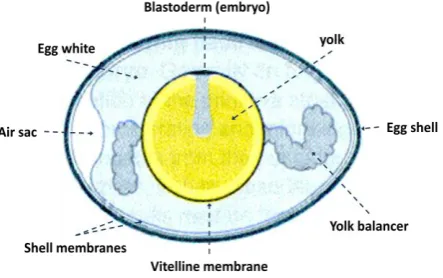
[image:13.595.190.412.169.308.2]Vertebrates share very similar developmental stages after fertilisation, from initial growth, emergence of important organising centres to large scale cell migrations leading to changes in form know as morphogenesis. In the chick embryo these changes take place geographically on the surface of the egg yolk, which can be seen macroscopically as a small opaque ring in any fertilised egg (Figure 1-1).
Figure 1-1: Basic structure of a chicken egg (Wolpert 2007). The common features are shown where the embryo is situated on top of the yolk as a small opaque disc.
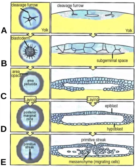
Cleavage. The first stage of development is concerned with growth as the newly fertilised cell (zygote) undergoes rapid cell divisions during the stage known as cleavage, that increases the number of cells in the embryo to form the a densely packed, multi layered group of cells called the Blastodisc, containing approximately 60,000 cells. At this point a cavity appears underneath the Blastodisc, separating it from the yolk to develop a subgerminal cavity, which is translucent and is given the name the area pellucida. Surrounding this translucent area is an opaque ring of cells that define the outer border of the embryo, given the name area opaca. As development proceeds a new layer of cell develops over the surface of the yolk called the hypoblast, that together with the topmost layer (now given the name the epiblast), completely surrounds the subgerminal space. It is on this surface, the epiblast, that the embryo proper will develop.
14 | P a g e
formation of the primitive streak it begins to regress, together with Hensen’s node posteriorly, with cells from the lateral epiblast converging on the streak and ingressing through it into the subgerminal cavity as mesenchyme cells (loosely connected), eventually forming the future mesoderm and endoderm germ layers (see Figure 1-2).
Figure 1-2: Illustration of the early stages in vertebrate embryonic development through to the formation of the primitive streak (Wolpert 2007). In the early stages the embryo undergoes rapid cell divisions to form the Blastodisc of approximately 60,000 cells (A). As development continues a subgerminal cavity appear separating it from the yolk (B), over which a unicellular of cells forms the hypoblast (C). The hypoblast together with the newly formed upper ceiling, the epiblast, now completely enclose the subgerminal cavity (D). At the posterior marginal zone a small crescent-like group of cells appears (D) the gives rise to a small condensation of cells known as Hensen’s node that begins to migrate over the surface of the epiblast to near the centre of the embryo, and as is does it leaves in its wake an invagination in the surface of the epiblast (E). Cells on the lateral epiblast converge on the streak and ingress through it to give rise to the future mesoderm and endoderm germ layers. The primitive streak, together with Hensen’s node make up the primary organiser of the developing organism, and define the primary body axes.
Neurulation. The regression of the primitive streak is coupled with the formation of the notochord, which one can refer to as the early backbone, which defines the so-called neural plate on which the early nervous system will develop. At the anterior end the notochord cells laterally convergence at the centre of the plate and begin to fold to form the early head process (encompassing the early brain) and the neural tube. Collectively one can visualise this process as the formation of the early central nervous system, with the early brain forming at the anterior and the development of the “backbone” being fuelled and organised by the regression of Hensen’s node.
Organogenesis And Beyond. Much of the rest of the development is concerned with development of internal organs and eyes, and largely signified by growth and enlargement until hatching.
A
B
C
[image:14.595.181.401.144.415.2]15 | P a g e
1.1.2 Mechanisms Of Cell Migration
Despite the large amount of experimental observations and data, there is still relatively little known about the forces and mechanisms that control the migrations of cells during early development of the chick embryo. The ability of a single cell to move is well understood, in terms of it physiology and bio-molecular signaling that motivates such movement. However in more complicated systems, such as during gastrulation in the chick embryo during formation of the primitive streak, a number of factors could be brought to bear. In such system there are large and diverse cell populations contained within densely packed medium exhibiting cellular flows, where it is not clear which cells are actively moving and which are being moved passively [9]. That is, some cells maybe actively moving in response to some signal, but in such a dense medium, there will inevitably other cells that are moving as a result of adhesive bonds with active cells, literally pushing and pulling surrounding cells. Further the forces and sources that cause such motion are also in question. However there seems to be agreement that in general, there are some fundamental mechanisms that describe cell motion/migration: cellular intercalation, cellular growth, apical constriction and chemotaxis.
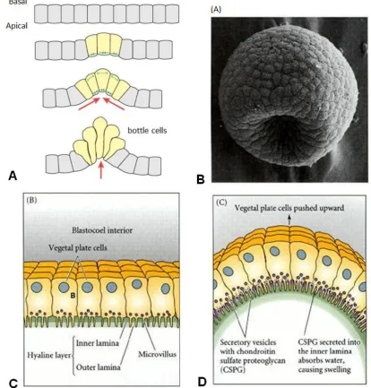
Apical Constriction
16 | P a g e
Figure 1-3: Apical constriction. (A) Illustration of a unicellular layer of cells undergoing constriction of the apical layer by causing surrounding cells move inwards as the local curvature increases. (B) Example of the apical constriction within the sea urchin (Lytechinus variegates) from Morrill and Santos 1985; C and D after Lane et al. 1993) as seen by scanning electron microscope. (C-D) Illustration of the structure and process leading to apical constriction.
[image:16.595.87.502.78.512.2]17 | P a g e
Cellular Intercalation
This is the process by which two groups of cells become spatially integrated. In one case there are two layers of cells stacked on top of each other, then by some mechanism the layers breaks the adhesive bonds between the cells their respective layers and begin to merge together thereby causing a radial cell flow or migration in the plain of intercalation. This type intercalation is referred to as radial intercalation, which typically reduces three-dimensional bodies of cells into a unicellular two-dimensional layer (Figure 1-4A).
Figure 1-4: Intercalation is the process by which two populations of cells spatially integrate to form new cellular structures. There are, in general, two ways this can happen: (A) multiple layers of cells can intercalate to form an expanding two-dimensional sheet, known as radial intercalation or (B) two-two-dimensional sheet converges bilaterally to form a single one dimensional row of cells, a process biologically referred to as convergent extension. (C) (Glickman N S et al. Development 2003;130:873-887) illustrates these principles within the development of the dorsal mesoderm of the zebra fish were the sub-panel (A) shows the actual cells of the embryo (B) the extension of the mesoderm and (C,D) coaxial views illustrating the shearing effects of the extension. The cells in sub-panels B, C and D are colour-coded according to their eventual fates with green the notochord-forming cells, dark blue adaxial cells, yellow and red cells associated with somite formation.
The second mechanism, Mediolateral intercalation, is similar to that of radial intercalation, however two layers appear to have a common one-dimensional interface, like sliding two pieces of paper together on a table (Figure 1-4B). This kind of intercalation occurs in many species during gastrulation, and is sometimes referred to as convergent extension, and is typical of axial extension in one-dimension such as in zebra fish development.
Chemotaxis
18 | P a g e
A
B
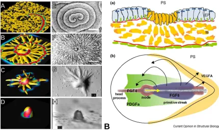
Figure 1-5: Panel A illustrates both simulated dynamics (sub-labelled A,B,C,D) and actual images of aggregations and mound formation (sub-labelled E,F,G,H). In sub-panel A-A the ameobae (yellow) are randomly distributed on a substrate and a spiral wave of cyclic adenosine monophosphate (cAMP) is initiated with colour-coded concentrations from high (red ~0.8) to low (0.0 blue). Sub-panel A-B illustrates streak formation as the amoebae aggregate towards the centre of the spiral as they are periodically excited by the wave eventually leading to the formation of the mound illustrated in sub-panel A-D. B: Current Opinion suggests that during gastrulation the primitive streak dynamics are controlled via chemo-repulsion by FGF8 and chemo-attraction of FGF4 giving rise to observed cell flows in and around the streak.
[image:18.595.87.518.74.329.2]19 | P a g e
1.2
Mathematical Modelling in Developmental Biology
1.2.1 Introduction
Much of the early work involved in developmental biology centered on observation, were given a model organism physiologists and biologists would make detailed notes and drawings of the various stages of development. From these detailed observations hypotheses were formed on the likely mechanisms or processes that drive the intricate stages of development. In the absence of genetic sequencing and/or advanced microscopy to identify regulatory networks of bio-molecules or bio-physical mechanisms, invariably these hypotheses would be investigated by interference with the normal developmental processes, such as by grafting, transplantation or even complete removal of whole sections of the embryo. Over the millennia a vast amount of data had been collected and catalogued from such experimentation, however much of the mechanisms involved in development biology still elude us to this day, primarily because of the incredible complexity that underlies even the most primitive biological organism.
It would appear that the classical approach of reductionism leads to us to an intractable problem. That is since the underlying complexity is so great, inevitably we would be lead to correlating an almost insurmountable number observations over vastly different spatiotemporal scales. This has lead to the development of fields such as System Biology that draw upon interdisciplinary research across the sub-fields of biology to draw conclusions at a more holistic level. Underpinning much of this research is the application of computational and mathematical models in a manner that captures the essential processes that give rise observable behaviour. In this respect, and quite ironically, mathematics does follow a reductionist approach, however, and as remarked by Murray [12]:
“The aim ... is not to derive a mathematical model that takes into account every single process because, even if this were possible, the resulting model would yield little or no insight on the crucial interactions within the (biological) system”
20 | P a g e
Within the remit of this thesis, we consider such systems in the context embryological development in the chicken. During early development of the central nervous system, the anteroposterior body axis extends, orchestrated and regulated by the organising centre Hensen’s node. It is known that this self-regulating behaviour allows for the node to move independently of the rest of the embryo, inducing pattern formation of the extending body axis controlled via intra-cellular signaling by the morphogen families of fibroblast growth factors (FGF) and retinoic acid (RA) [5, 7]. The central question we seek to answer, and indeed model, is what mechanism accounts for this regulation that allows the node to move? As we have suggested in the previous section there several mechanisms that can account migrations of tissue or cells within the embryo, however we propose that a single chemotactic mechanism is responsible. Thus at the heart of this project is the problem associated with understanding the origins and dynamics of experimentally observed morphogens, and the resultant dynamical behaviour of the node in terms uniform motion.
For the remainder of this section we shall consider some of these mathematical models as they contribute to the project at hand, namely embryonic development within the chick egg, with a view to understanding methods of cell migrations in around Hensen’s node leading to its regression.
1.2.2 Modeling Morphogen Concentrations and Pattern Formation
The term morphogen, as coined by Turing [16], speaks of a bio-chemical that can be involved in change of form and shape within developing biological systems. These changes can be associated with reorganisation of cellular structures whereby cells migrate into new positions, typically during development of the early body plan of the organism, but continue throughout the developmental process. Morphogens are also known to be involved in patterning that is not necessarily connected with reorganisation, but with molecular cell differentiation, whereby a group of cells are exposed to the distribution of one or more morphogens that trigger differentiation of cells within the group according to level of the morphogen they exposed to. The resultant type after differentiation is dependent on the developmental history of each cell, so that coupled with the exposure to the morphogen, spatial patterns in cell type will emerge.
21 | P a g e
French Flag Model Of Pattern Formation
The interpretation and subsequent differentiation according to the spatial positioning within the morphogen concentration, was termed positional information by Wolpert [15] and is characterised in his French flag problem as illustrated in Figure 1-6.
Figure 1-6: A group of cells exposed to a morphogen concentration can differentiate according to the exposure at specific gradients or thresholds of the morphogen. Assume a homogeneous linear arrangement of cells of width . At gradients in the concentration, and , differentiation can give rise to spatial patterns of different cell types corresponding to bands of the colours blue, white and red at exact position over the group, , and .
In the classic setting Wolpert suggested that a simple linear passive distribution of a morphogen over the group of cells of length , that at thresholds in its concentrations ( ), could signal differentiation of cells, defining differentiation threshold boundaries. Cells in the group with a concentration greater than the threshold for would differentiate to become blue, while below for would become white and below for red, giving a simplistic model:
( ) ( ) (1.1)
with the concentration of the morphogen, the diffustion coefficient and and the values at the boundaries representing source and sink concentrations respectively, implying a linear solution (Figure 1-6A):
( ) (1.2)
While such a formulation allows for size invariance, implying we can double the size of the group, to , and similar pattern would result, albeit slightly larger, such distributions do not correlate well with experimental observations. However a similar result can be achieved by assuming a non-linear distribution with active diffusion (Figure 1-6B):
( )
|
|
(1.3)
where the concentration decays proportional to its own concentration with rate , and its production is given by the characteristic function:
22 | P a g e
with an arbitrary positive production constant defined in the domain of size . In this setting it assumed that the cells within the group are sensitive not to threshold value of the morphogen, but its gradient ( ). However it should be clear that this second model does not possess size invariance, as the distribution of the morphogen in this case is only dependent on the diffusion coefficient and the decay rate . This implies that if we double the size of them medium in this case, the relative horizontal dimensions of each part of the flag would differ.
In either case the French flag problem illustrates quite elegantly how relatively simplistic mechanisms can bring about complex pattern formation, due to the dynamics of a single morphogen. In the next section we shall see that adding a secondary morphogen to the system can lead spatially stable patterns in the morphogens.
Pattern Formation in a Two Component System
In a landmark paper “The Chemical Basis of Morphogenesis” Alan Turing [16] proposed that spatially stable patterns could occur in a two-morphogen system if they possessed different diffusion rates. Such systems have come to be known as reaction-diffusion systems. In principle there are two morphogens, one the activator, , and the second the inhibitor, . The activator exhibits an autocatalytic reaction that self-enhances its own production, while simultaneously catalysing the production of the inhibitor. The inhibitor also has an autocatalytic reaction but in addition acts to down-regulate, or catalyses decay, of the activator. In its most general form, such a system can be given by the following system in one-dimension:
( ) (1.5)
( ) (1.6)
The coefficients and are constants representing the rate of diffusion, and ( ) and ( ) the associated kinetics terms, that assumed to be both a function of the activator and inhibitor concentrations, collectively describing the interdependent rates of production and decay.
23 | P a g e
Figure 1-7: Examples of pattern forming behavior in a Fitzhugh-Nagumo type reaction-diffusion system (images sourced from Wikipedia). Depending on the reaction kinetics of the equation various patterns can form such spiral waves (A) circular propagating waves (B) or stationary spots (C) and in hysteresis where from a seemingly chaotic (noisey) system distributed irregular patterns can forms.
For example the well-known Fitzhugh-Nagumo (a qualitative generalization of the Hodgkin-Huxley model) model involves excitable or fast variable, typically given as a non-linear cubic equation, and a slow refactory variable, typically linear as a model of squid axon induction of excitation. The form of these equations have become widespread in the modeling of reaction-diffusion system due to the variety of travelling, propagating or stationary patterns can result (Figure 1-7) such spiral waves, pulsating or stationary spots and spatially distributed patterns (See proceeding section Figure 1-6).
1.2.3 Chemotaxis
Chemotaxis is a phenomenon whereby somatic cells, bacteria and other single-cell organisms direct their movements according to certain chemicals in their environment. History of chemotaxis research is indeed well known. Migration of cells was detected from the early days of the development of microscopy but erudite description of chemotaxis was first made by TW. Engelmann and WF. Pfeifer in bacteria and H.S. Jennings in ciliates. The significance of chemotaxis in biology and clinical pathology was widely accepted in the 1930s [17]. Chemotaxis is important for bacteria to find food (for example glucose) by swimming towards the highest concentration of food molecules, or to flee from poisons (for example phenol). In multicellular organisms, chemotaxis is critical to early development (for example the movement of sperm towards the egg during fertilization) and subsequent phases of development (for example the migration of neurons and lymphocytes) as well as in normal function. In addition, it has been recognised that mechanisms that allow chemotaxis in animals can be subverted during cancer metastasis.
24 | P a g e
cancer metastasis. It has high significance in the early phases of embryogenesis as development of germ layers is guided by gradients of signal molecules [18].
The use of mathematical techniques for classification and understanding of the ever-growing amount of experimental data and possible help in designing new experiments is now more profound than ever. Recently, mathematical modelling played an growing role in biological studies in general and in particular, in developmental biology. Mathematical modelling in developmental biology has an important role in helping us discover biophysical mechanics driving the development. It is a unique tool which allows a rigorous check of hypotheses concerning these mechanisms as they emerge from the experimental observations. Several mathematical models of chemotaxis were developed depending (among which) on the type of
a) migration (for examples the basic differences of bacterial swimming, movement of unicellular eukaryotes with cilia/flagellum and amoeboid migration),
b) assay systems applied to evaluate chemotaxis (to see incubation times, development and stability of concentration gradients) and
c) other environmental effects possessing direct or indirect influence on the migration (lighting, temperature, magnetic fields, etc.).
Other publications written in genetics, biochemistry, cell physiology, pathology and clinical sciences can also incorporate data about migration or especially the chemotaxis of cells. A curiosity of migration research is that among several works investigating taxes (for examples thermotaxis, geotaxis and phototaxis), chemotaxis research shows a significantly high ratio, which point to the underlined importance of chemotaxis research both in biology and medicine [17]. For chemotaxis, a mathematical description for it requires a model to describe the cells ability to sense a gradient of ambient chemo-attractant and its interaction with a physical model of cell migration. It is also now appreciated that it is important to model the feedback from the evolving cell shape and the intra and extra cell signalling pathways which lead to directed cell motion. The computational challenge therefore involves the solution of partial differential equations (PDEs) on evolving surfaces where the computed solution state is used to derive movement and changes in cell shape.
25 | P a g e
An individual cell path can result in an average cell flux which is proportional to the macroscopic chemical gradient. If we let ( ) denote the density of cells centred at and ( ) the net flux of cells per unit time in the direction of increasing . Then the dependence of cell density ( ) on position and time is described by the differential equation:
( ) (1.7)
where the vector flux is given by:
(1.8)
The first term is the diffusion term, describing the non-chemotactic, random motion of cells, and the second term describes the chemotactic response.
Chemotaxis has been used in the detailed study of the developing population of Dictyostelium discoideum (Dd) amoebae. This biological organism cooperates with and shows striking social behaviour when they are deprived of food. The starving cells then communicate by means of chemical signal to synchronise their otherwise random and unorganised movement.
The molecular machinery for cell motility is currently best understood in Dd. This is because it is an organism which spends most of its life as a chemotactic amoeboid phagocyte but which also uses chemotaxis to form a multicellular organism during subsequent stages of development. In this process of transformation, there is both production of and a chemotactic response to cyclic adenosine – monophosphate (cAMP); the result is aggregation [19].
Aggregation of Dd amoebae is an example of a phenomenon whereby the wave of excitation can change the properties of excitable media and cause the formation of spatial patterns. The monolayer of the starving amoebae is an excitable medium which conducts excitation waves of the intracellular mediator i.e. the cAMP. Since cAMP is a chemotactic attractant for the amoebae, the waves of cAMP cause motion of the amoebae. As a result of this motion amoebae are organized into streams which usually form branching radial multicellular structures. There are two major types of cAMP sources forming aggregates: a point source and a spiral wave. Figure 1-8: shows streams which were induced by a spiral wave of cAMP.
26 | P a g e
The process of aggregation of Dd amoebae was numerically studied in a continuous model and thus the reaction-diffusion model [19] was proposed for the simulation of the process. The model is based on FitzHugh-Nagumo-type equations for cAMP waves and a continuity equation for amoebae motion. The process of aggregation induced was simulated by a periodic point source and by a spiral wave. It was shown that an aggregation pattern is formed as a result of front instabilities due to dependence of wave velocity on density of amoebae. This instability can also result in formation of wave breaks and generation of spiral waves.
For calculations, the following model was used:
( ( ) )
( ( ) )
(1.9)
The first two equations are a Fitzhugh-Nagumo model which describes the propagation of cAMP waves. represents the extracellular concentration of cAMP and , the refactory period. Instead of ordinary cubic function, ( ), in the second equation, the piecewise linear function is used instead:
( ) {
( )
( )
(1.10)
( is infinite, ( ) is only defined on the interval ). It was suggested that in normal conditions, the production and decay of cAMP are proportional to the cell density ( ).
The third equation in (1.9) describes the chemotactic motion of amoebae. is the local concentration of amoebae, and ( ) is their motility. In the model (as ), reaches its maximum at and decreases to , with increasing . Biologically, this means that cells move if they are not refractory (i.e. not able to respond to additional stimulation).
27 | P a g e
The reaction-diffusion model proposed describes fairly well the aggregation process in natural population of Dd. The aggregation pattern obtained by numerical simulation looks similar to the pattern in amoebae populations (Figure 1-8). In addition, the technical features which makes Dd amoebae attractive as a model includes [9]:
a) The cells exist as a homogeneous population in culture,
b) They can be induced by physiologic stimuli to undergo normal morphogenesis in vitro thus permitting direct observation of the role of chemotaxis in organogenesis,
c) Cells can be grown in suspension culture to high density to generate kilogram quantities of material for biochemical analysis,
d) Amoeboid cells are haploid and are readily manipulated by molecular genetic techniques and
e) The physiological response to chemotactic stimulation is synchronous in a cell population and can, therefore, be correlated with biochemical measurements.
1.2.4 Numerical Methods
Much of the analysis of this thesis involves the development of two numerical/computational tools: BioCellSim and BioChemSim. BioCellSim, as its name suggests is a two-dimensional cell-centered computational model based of the Cellular Potts Model of Glazier & Graner [20], which we implemented and modified to satisfy our modelling needs. BioChemSim on the other hand is an entirely novel model we derived for simulation of chemical and chemotactic dynamics. In this section we wish to briefly set out the numerical methods we employed in these models, primarily in terms of reaction-diffusion. It should be noted that we will not be discussing here the CPM per-se, rather we will only outline the numerical implementations of the chemical models we use. In all of our models we used a forward-time centered-space (FTCS) explicit Euler finite differencing scheme.
Numerical Reaction-Diffusion Equations
In all numerical modelling of chemicals we can see, both one and two-dimensions, that our diffusion equation is given as a standard parabolic equation with added kinetics expressed in (1.11) as ( ). From the point of view of deriving a numerical model, the only difference between one and two dimensions is in the expression for the Laplacian differential operator , where in one dimension it takes the form ⁄ and in two dimensions ( ⁄ ⁄ ). The kinetics term can be considered equivalent in both models and as it is linear it does not affect the derivation of the numerical form, thus we can state the governing equation for both one and two dimensional models as:
( )
( ) ( ) ( ) ) (1.11)
28 | P a g e
In other words the spatio-temporal derivatives can be seen as taking approximations for small perturbations in both space and time. In this way we can see that we can see that we can represent derivatives as Taylor series expansions about these small differences/perturbations, which can be visually illustrated as stencils in Figure 1-9.
Figure 1-9: Numerical stencils for one and two-dimensional explicit Euler, forward-time centered-space differencing scheme in one dimension (A) and two dimensions (B).
Considering the spatial variation, , in one-dimension of the chemical concentration ( ) due to diffusion at a discrete numerical grid point , we can approximate this by the Taylor expansion:
( ) ( ) ( ) ( )( ) ( ) (1.12)
and
( ) ( ) ( ) ( )( ) ( ) (1.13)
If we now take the superposition of (1.12) and (1.13) and rearrange we find:
( ) ( ) ( ) ( )
( ) (1.14)
is an approximation to the second order derivative with respect to space, , where it should be clear that we can perform an equivalent derivation for a second spatial dimension, , as:
( ) ( ) ( ) ( )
( ) (1.15)
Then by superposition of (1.14) and (1.15) we can an approximation to the Laplacian differential operator in two-dimensions as:
( ) ( ) ( ( ) ( ) ( ) (1.16)
( ) ( ) ( ) )
where for simplicity we have assumed that the grid is isotropic, and in one-dimension as:
( ) ( ) ( ( ) ( ) ( )
29 | P a g e
The representation of the temporal derivative can be derived by equivalent means and be shown to be of the form:
(
( ) ( )
) (1.18)
Now if we substitute (1.16) and (1.18) in (1.11), and make a symbolic change of ( ) then we
have:
( ) (1.19)
which after simplification we find the FTCS finite differencing approximation to (1.11) in two dimensions:
{ ( )} (1.20)
and in one-dimension:
{
( )} (1.21)
Stability of FTCS Numerical Scheme
The stability, or instability, of the numerical schemes given by (1.20) and (1.21) is seen as a function of the numerical error associated with the scheme and is attributed to the rate at which spatial information contributes to each grid point from time to time . In each time step, , in (1.20) or (1.21) the contributing information for a grid point, , comes from ,
and . If neglect
the kinetics terms ( ) in (1.21) and re-write it as:
( )
(1.22)
where , the standard condition for stability is given by for (1.22). Formally we can derive the condition for stability by the method of Von-Neumann stability analysis, where we assume that coefficients of the difference equation are varying so slowly in space and time as to make them approximately constant. In this way we can assume that the eigenmodes of the difference equation are all of the from
30 | P a g e
Substituting (1.23) into (1.22) we find:
( ) ( )
( )
( )
(1.24)
now using the identities:
( ) ( ) ( ) (1.25) we can rewrite (1.25) as
( ) ( ) (1.26)
where we have written ( ) which is referred to as the amplification factor, and therefore to
satisfy | ( )| we require:
| ( )| , (1.27)
for the numerical scheme to remain stable, and this conditions is known as the famous Courant condition. In essence (1.26) states that for any specification of the we are required to ensure that is set such that the condition in (1.27) holds.
Accuracy Of Numerical Scheme
We shall only note here the method we have used to ensure the accuracy of our simulations and we will only be considering details that warrant a justification for our simulations. The accuracy, or more accurately, the inaccuracy of the numerical scheme, can be seen to be caused two different problems: boundary size and incorrect specification or spatio-temporal scales used.
Boundary size is important in that in a diffusive scheme, if the boundary of the domain of the problem are set too close, then the numerical simulation will not (literally) have enough space to for the solutions to saturate properly. In the context our problem, if boundary is too close to the domain of transcription, given in one-dimension as a segment and in two dimension a disk, then the chemicals will have a limited into which they can diffuse, and so the resultant chemical profiles will not be accurate. To account for this problem, we can simply ensure that the boundary size is large enough, however in practice it is not readily clear what “large enough” translates to in any given simulation. Our solutions was quite simple, when obtaining results from simulations we always sought to check the results by doubling the size of the medium to determine if the boundary was having any appreciable effect.
31 | P a g e
would increase the segment/disk twice, double the spatial step and divide the temporal step by a factor of four and adjust boundaries dimensions if need be. If we found a less than 3% difference in numerical results we would accept this as being reasonably accurate.
1.3
The Cellular Potts Model
The CPM has its origins in mathematical physics as a mathematical model used to study phase transitions that occur in physical systems. While not self-evident why research into phase transitions allows us to model cellular phenomena, we shall see in the following sections how (and a common practice in science) the development of a model in one discipline can have broad applicability in others. In terms of the CPM this originates with the work of Ernst Irving, in the study of magnetic properties of ferromagnetic materials. Therefore we shall begin at the beginning, so to speak, and show the development of the Ising Model into CPM we will be using for the rest of this chapter.
1.3.1 The Ising Model
The Ising model was developed by Ernst Ising for his 1925 PhD Thesis, in an attempt to derive a mathematical model whose solution could predict spontaneous magnetization in ferromagnetic materials such as iron, nickel, cobalt or their alloys. This spontaneous change in behaviour, or “phase transition” in these materials from paramagnetic to ferromagnetic was/is of significant interest, as the production of magnets on an industrial scale clearly has large ranging applications throughout all sectors of industry and society. While there was a great deal of intuition for what phase transitions were, and even how they occur, there was no mathematical tools/models that could demonstrate this analytically. Thus Ising’s work was a first attempt to derive a closed-from analytical expression that could describe conditions, using weak assumptions, on system parameters for such phase transitions to occur. In Ising’s original work in one-dimension (referred to as one-one-dimensional chains, the term Ising Model was coined by Perierls [21]) he failed to demonstrate such transitions which, in very broad terms, he incorrectly concluded that similar results would occur in higher dimensions. It wasn’t until nearly a decade later through the work of Perirels [21] and Kramers & Wannier [22] that it was shown that a phase transition can occur in two-dimensions, and several years later Onsager [23] derived an analytical solution to the model in the absence of an external magnetic field, the so called zero-field.
32 | P a g e
notwithstanding variations in surrounding atmospheric pressure or temperature (an idealised system) mark precise conditions for the transition from liquid to solid or liquid to vapour. These changes manifests as a discontinuous change in the density of the water, which is given to be the first derivative of the free energy with respect to the chemical potential, and therefore a first-order transition.
For Ising’s work, magnetism, we know from classical electrodynamics that spinning electrically charged bodies will produce a magnetic dipole with poles having equal magnitude and opposite polarity. In terms of atoms the concept of “spin” is given to be a collective analogy of the angular and orbital moment of electrons about the nucleus. Clearly if two locally and equally interacting atoms have opposite spin, necessarily implying opposite polarity, then the net magnetic moment will be zero. Therefore if a material is to exhibit a useful measurable magnetic field, the configuration of atoms within the material must favour interactions between atoms with equal polarity/spin; the greater the degree of alignment, the greater the net force. Practically this is achieved by re-organising the materials microcrystalline structure, by heating the material and exposing it to a powerful magnetic field. As the magnetic field is reduced, and assuming the temperature of the material is at a critical (constant) value (less than the materials Currie point), the material will undergo a ferromagnetic phase transition to exhibit spontaneous magnetisation. In this sense the magnetisation of the material is given by a first derivative of the free energy with respect to the applied magnetic field, which is a continuously increasing function as the temperature is lowered below its Currie point. However the magnetic susceptibility of the material is given by the second derivate, which exhibits a discontinuity in the onset of spontaneous magnetisation, and therefore is described as a second-order phase transition.
33 | P a g e
Figure 1-10: Illustrations of Ising lattices ( ) in one, two and three spatial dimensions. The Ising model in its inception was described by the arrangement of equally spin states, , on a line (A), however the model can be easily generalised to higher dimensions where in two dimensions we have a grid (B) and in three dimension we have cube (C).
Local interactions on can now be seen as what one might term as nearest neighbour interactions, or first order interactions, that occur between sites that are at most one lattice site away from the site of interest . It is possible to consider higher order interactions, but for the rest of this work only first order interactions will be considered. If we let be the dimension of the then we can see that for a given there will be interactions (or local atomic bonds) forming a stencil of interacting sites as illustrated in Figure 1-11.
Figure 1-11: Energy is computed on by interactions with nearest neighbour sites about the site of interest . These nearest neighbour interactions can be defined in higher dimensions and form stencil of sorts that can be considered as the smallest computational unit of energy on when calculating the Hamiltonian of the system.
These interaction stencils are taken to be the smallest unit of energy computation and they form the basis of the Hamiltonian, of the system. That is gives us function from which we determine the current energy state of . At this point we should note that this highlights Ising’s largest assumption for the model, as generally speaking a Hamiltonian gives the total energy state of a system, whereas here the assumption is that only first order interactions contribute to the final state. Therefore for Ising introduced the following Hamiltonian:
( ) ∑ ( ) ∑ ( ) (1.28)
which expresses the summation over all lattice sites on ( ).
34 | P a g e
orientation of the magnetic field should tend to align states, and therefore should contribute to the minimization of energy.
As suggested earlier, an important aspect of phase transitions is that changes in the qualitative behaviour of the thermodynamic system manifest as abrupt, discontinuous changes, which in the case of ferromagnetic transitions is described as spontaneous magnetisation. We can infer from this description that transitions are not deterministic in nature, moreover they are characterised by stochastic processes, which brings us to the central object used by the Ising model, the partition function from statistical mechanics:
( ) ∑ ( )
(1.29)
where parameter with the absolute temperature and is the Boltzmann factor that relates temperature and energy at the microscopic particle level, and the minus sign suggest that lower energy states are preferred.
In general (1.29) is the sum over all configuration microstates on which for a lattice of sites equates to possible spin state configurations. Its use becomes apparent when we consider the probability of one such a spin state configuration, , that is a specific assignment of states , then the probability of occuring is given by the so-called Boltzmann probability distribution:
( ) (
)
(1.30)
More generally (1.30) encodes statistical information about the thermodynamic features of the system, such as heat, magnetism, etc. For example the expected internal free energy is given to be the weighted probability:
( ) ∑ ( )
( )
(1.31)
which we can see can be expressed as the derivative with respect to the temperature of the system
( )
(1.32)
This brings us to the central question in the Ising model: if we define the free energy per lattice site as ( )
( ) (1.33)
where is called the thermodynamic limit, then Ising sought a closed form analytical solution for ( ). The reasoning for this is that if phase transitions do occur, then they would manifest as discontinuities in or one of its derivatives. However there is no guarantee that such a limit exists.
35 | P a g e
1.3.2 The Potts (Clock) model
In this section we acknowledge the work of Renfrey Potts in generalizing the Ising model in his 1952 PhD thesis under the supervision of C. Domb. The Potts Model, as it has now come to be known, was first suggested to Potts by his supervisor Cyral Domb for his PhD thesis. The principle was that the Ising model could be generalized to more than two spin states. That is, can phase transitions be found in lattice where there are different spin states? As stated earlier, the Ising model for was solved for a zero field [23] and indeed the Potts Model is equivalent to the Ising Model for this value of . The problem was to consider the spins as equally spaced spins confined to the plane or as Domb suggested,
spins equally spaced around a circle, with angles
(1.34)
which gives symmetric spin states, which lead to the construction sometimes being referred to as the Clock Model, as one can see in Figure 1-12.
Figure 1-12: Potts’s extension of the Ising model was to suggest that spin states could be generalised so as to allow an arbitrary number of states to occur. The construction of this model assumed that the spin states can be considered as -symmetric angular subdivisions of a two-dimensional circle, with each state given by an angle where . Thus this model was sometimes referred to as the clock model for its similarity to a clock face, illustrated above for and . One should note that corresponds to the so-called Ising value as for this value the Potts model is equivalent to the Ising’s.
In addition, Domb suggested the following interaction Hamiltonian, ∑ ( )
(1.35)
where ( ) is the angle between two spins at neighbouring sites, and on the lattice and is the strength of the interaction. The factor under the summation, , is taken to be shorthand for the summation over all nearest neighbours. However, in solving the problem, Potts used the following simplified Hamiltonian:
∑ ( )
(1.36)
36 | P a g e
1.3.3 The Extended Large-q Potts Model
In the previous discussion the main efforts in the development of the Potts model were concerned with analytical techniques, to derive closed-form solutions that can describe statistical properties of the material. At this juncture the development diverges and the models evolution is now concerned with the qualitative rather than the quantitative. To understand this let us refresh with a mental picture of what come so far. If we consider the Ising (and Potts) model, the spontaneous magnetisation is the occurrence of a dominant set of co-aligned atomic spin states that lead to a net permanent magnetic moment in the material. However if we were to visualise such a configuration, then we would see that rather than a uniform distribution of alignments, we would see small pockets of moments irregularly distributed over the materials microcrystalline ( ) structure as illustrated in Figure 1-13.
Figure 1-13: Graphical representations of the Ising model for probabilistic distribution of two-dimensional an lattice (courtesy of Linas Vepstas 2006). For possible states implies a pixel image with each pixel representing a single spin state. The colours are chosen as black such that the probability of a spin state is not likely to occur as, ( ) , grey such that the state has a borderline probability of acceptance, ( ) , and white for ( ) implying state is highly likely.
This perceived irregularity is a function of the degeneracy of the ground/spin states in the model which is prescribed by which clearly for low , as is the case for the Ising value , is what one might expect given that random spin flips occur without regard spin orientations of it neighbours beyond the Boltzmann probability. However the situation becomes more interesting when we consider higher degeneracy for , as suggested by Anderson and Grest [24].
[image:36.595.225.373.246.401.2]37 | P a g e
The latter observation is central to the development of the CPM, specifically Anderson et al made the distinction that energy of the system is a function of temperature, but more importantly, energy fluctuations are only significant at nucleation sites. In terms of the Potts model this is reflected in their modified Hamiltonian:
∑ ( ( ))
(1.37)
where again ( ) is the Kroenecker delta function, is the interactions energy and is the summation over all nearest neighbours. Clearly (1.37) is zero when and when . Like the Ising/Potts models they suggested that consists of regularly arranged spin states where , however in addition each state can have multiplicity such that leading to a degeneracy of . This degeneracy of states on , coupled with (1.37) leads to homogenised domains of like states or as they put it “...higher ground-state degeneracy had an effect on the growth kinetics, the microstructure, and the topology.” . This can clearly be seen when we consider domain-growth for increasing (Figure 1-14), where for low the domains are irregular and asymmetric, but as is increased the grain structure becomes more pronounced and equiaxed.
Figure 1-14: Simulations of grain structures growing and becoming more pronounced and equiaxed as the degeneracy, , of the spin states increases. The solid black curves represent the boundaries between domains of like spin states, on which energetic interactions take place representing the physical phenomena in real alloys of nucleation of precipitates that takes place during quenching from above the alloy’s melting point to [24]. Simulations illustrated above show that after quenching we can see clearly that as the degeneracy increases from to the topology of the structure exhibits clear grain like structures.
1.3.4 The Monte Carlo Method.