Convergence guarantees for a class of
non-convex and non-smooth optimization problems
Koulik Khamaru? [email protected]
Martin J. Wainwright?,†,‡ [email protected]
Department of Statistics?
Department of Electrical Engineering & Computer Sciences† University of California Berkeley
Berkeley, CA 94720-1776, USA Voleon Group‡
Berkeley, CA
Editor:Alexander Rakhlin
Abstract
We consider the problem of finding critical points of functions that are convex and non-smooth. Studying a fairly broad class of such problems, we analyze the behavior of three gradient-based methods (gradient descent, proximal update, and Frank-Wolfe update). For each of these methods, we establish rates of convergence for general problems, and also prove faster rates for continuous sub-analytic functions. We also show that our algorithms can escape strict saddle points for a class of non-smooth functions, thereby generalizing known results for smooth functions. Our analysis leads to a simplification of the popular CCCP algorithm, used for optimizing functions that can be written as a difference of two convex functions. Our simplified algorithm retains all the convergence properties of CCCP, along with a significantly lower cost per iteration. We illustrate our methods and theory via applications to the problems of best subset selection, robust estimation, mixture density estimation, and shape-from-shading reconstruction.
1. Introduction
Non-convex optimization problems arise frequently in statistical machine learning; exam-ples include the use of non-convex penalties for enforcing sparsity (Fan and Li, 2001; Loh and Wainwright, 2013; Wainwright, 2019), non-convexity in likelihoods in mixture model-ing (Yan et al., 2017), and non-convexity in neural network trainmodel-ing (Li and Yuan, 2017). Of course, minimizing a non-convex problem is NP-hard in general, but problems that arise in machine learning applications are not constructed in an adversarial manner. Moreover, there have been a number of recent papers demonstrating that all first (and/or second) order critical points have desirable properties for certain statistical problems (e.g. Loh and Wainwright 2013; Ge et al. 2017). Given results of this type, it is often sufficient to find critical points that are first-order (and possibly second-order) stationary. Accordingly, re-cent years have witnessed an explosion of research on different algorithms for non-convex problems, with the goal of trying to characterize the nature of their fixed points, and their convergence properties.
c
There is a lengthy literature on non-convex optimization, dating back more than six decades, and rapidly evolving in the present (e.g., see Tuy 1995; Hartman 1959; Horst et al. 2000; Lanckriet and Sriperumbudur 2009; Yuille and Rangarajan 2003; Lee et al. 2016; Bolte et al. 2014; Panageas and Piliouras 2016; Lipp and Boyd 2016; Cartis et al. 2010; Attouch et al. 2010; Gotoh et al. 2017). Perhaps the most straightforward approach to obtaining a first-order critical point is via gradient descent. Under suitable regularity conditions and step size choices, it can be shown that gradient descent can be used to compute first-order critical points. Moreover, with a random initialization and additional regularity conditions, gradient descent converges almost surely to a second-order station-ary point (e.g., Lee et al. 2016; Panageas and Piliouras 2016). These results, like much of the currently available theory for (sub)-gradient methods for non-convex problems, involve smoothness conditions on the underlying objectives. In practice, many machine learning problems have non-smooth components; examples include the hinge loss in support vector machines, the rectified linear unit in neural networks, and various types of matrix regular-izers in collaborative filtering and recommender systems. Accordingly, a natural goal is to develop subgradient-based techniques that apply to a broader class of non-convex functions, allowing for non-smoothness.
The main contribution of this paper is to provide precisely such a set of techniques, along with non-asymptotic guarantees on their convergence rates. In particular, we study algorithms that can be used to obtain first-order (and in some cases, also second-order) optimal solutions to a relatively broad class of convex functions, allowing for non-smoothness in certain portions of the problem. For each sequence {xk}k≥0 generated by one of our algorithms, we provide non-asymptotic bounds on the convergence rate of the gradient sequence {k∇f(xk)k2}k≥0. Moreover, for functions that satisfy a form of the Kurdaya- Lojasiewicz inequality, we show that our methods achieve faster rates.
Our work has important points of contact with a recent line of papers on algorithms for non-convex and non-smooth problems, and we discuss a few of them here. Bolte et al. (2014) developed a proximal-type algorithm applicable to objective functions formed as a sum of smooth (possibly non-convex) and a convex (possibly non-differentiable) function. Some recent work by Xu and Yin (2017) extended these ideas and provided analysis for block co-ordinate descent methods for non-convex functions. Hong et al. (2016) analyzed the ADMM method for non-convex problems, whereas in other recent work (An and Nam, 2017; Wen et al., 2018), the authors proposed a proximal-type method for non-convex functions that can be written as a sum of a smooth function, a concave continuous function and a convex lower semi-continuous function; we also analyze this class in one of our results (Theorem 2).
Sriperum-budur, 2009), it can be slow in many situations due to its double loop structure. One outcome of the analysis in this paper is a single-loop proximal-method that retains all the convergence guarantees of CCCP while—as shown in our experimental results—being much faster to run.
1.1. Problem setup
In this paper, we study the problem of minimizing a non-convex and possibly non-smooth function over a closed convex set. More precisely, we consider optimization problems of the form
min x∈C
n
g(x)−h(x) +ϕ(x)
| {z }
f(x)
o
, (1)
where the domainCis a closed convex set. In all cases, we assume the functionf is bounded below over domainC, and that the functionhis continuous and convex. Our aim is to derive algorithms for problem (1) for various types of functions g andϕ.
Structural assumption on functions g and h
(a) Theorems 1 and 4 are based on the assumption that the function g is continuously differentiable and smooth, and that the functionϕ≡0.
(b) In Theorems 2 and 5, we assume that the functiongis continuously differentiable and smooth, and that the function ϕis convex, proper and lower semi-continuous.1 (c) Theorem 3 focuses on the case in which the function g is continuously differentiable,
and the functionϕ≡0.
The class of non-convex functions covered in part (a) includes, as a special case, the class of differences of convex (DC) functions, for which the first convex function is smooth and the second convex function is continuous. Note that we only put a mild assumption of continuity on the convex functionh, meaning that the difference functiong−hcan be non-smooth and non-differentiable in general. In particular, for any continuously differentiable function h and any smooth function g, the difference function f = g−h is non-smooth. Furthermore, if we take the function h≡0, then we recover the class of smooth functions as a special case.
1.2. Overview of our results
• Our first main result (Theorem 1) provides guarantees for a subgradient algorithm as applied to the minimization problem (2), to be defined in the sequel, when constrained to a closed convex setC. We provide convergence bounds in terms of the Euclidean norm of
the subgradient and show that our rates are unimprovable in general. We also illustrate some consequences of Theorem 1 by deriving a convergence rate for our algorithm when applied to non-smooth coercive functions; this result has interesting implications for polynomial programming. We also provide a simplification of the CCCP algorithm, along with convergence guarantees. In Corollary 3, we argue that our algorithm can escape strict saddle points for a large class of non-smooth functions, thereby generalizing known results for smooth functions.
• Our second main result (Theorem 2) provides convergence rates for a proximal-type algorithm for problem (1). In Section 4.3, we demonstrate how this proximal-type algorithm can be used to minimize a smooth convex function subject to a sparsity constraint. We demonstrate the performance of this algorithm through the example of best subset selection.
• In Theorem 3, we provide a Frank-Wolfe type algorithm for solving optimization prob-lem (17), and we provide a rate of convergence in terms of the associated Frank-Wolfe gap.
• Finally, in Theorems 4 and 5, we prove that Algorithms 1 and 2, when applied to functions that satisfy a variant of the Kurdaya- Lojasiewicz inequality, have faster con-vergence rates. In particular, the concon-vergence rate in terms of gradient norm is at least
O(1/k) – whereas the worst case rate for general non-convex functions is O(√1
k). We also provide examples of functions for which the convergence rate isO(1/kr) withr >1. In Theorem 6, we characterize the class of functions that can be written as a difference of a smooth function and a differentiable convex function.
Section 4 is devoted to an illustration of our methods and theory via applications to the problems of best subset selection, robust estimation, mixture density estimation and shape-from-shading reconstruction.
Notation: Given a setC ⊂ Rd, we use int(C) to denote its interior. We usekxk 2, kxk1 and kxk0 to denote the Euclidean norm, `1-norm and `0 norms, respectively, of a vector x∈Rd. We say that a continuously differentiable function g is M
g-smooth if the gradient
∇g is Mg-Lipschitz continuous. In many examples considered in this paper, the objective function f is a linear combination of a differentiable function g and one or more convex functions h and ϕ. With a slight abuse of notation, for a functionf =g−h+ϕ, we refer to a vector of the form ∇g(x)−u(x) +v(x), where u(x) ∈ ∂h(x) and v(x) ∈ ∂ϕ(x), as a gradient of the function f at point x — and we denote it by ∇f(x); here, ∂h(·) and ∂ϕ(·) denote the subgradient sets of the convex functions h and ϕ respectively. We say a point x is a critical point of the function f if 0 ∈ ∇f(x). For a sequence
ak k≥0, we define the running arithmetic mean Avg ak
as Avg ak
: = 1kP`=k+1
`=0 a`. Similarly, for a non-negative sequence ak k≥0, we use GAvg ak: = (
k
Q
`=0
a`)k+11 to denote the running
2. Main results
Our main results are analyses of three algorithms for this class of non-convex non-smooth problems; in particular, we derive non-asymptotic bounds on their rates of convergence. The first algorithm is a (sub)-gradient-type method, and it is mainly suited for unconstrained optimization; the second algorithm is based on a proximal operator and can be applied to constrained optimization problems. The third algorithm is a Frank-Wolfe-type algorithm, which is also suitable for constrained optimization problems, but it applies to a more general class of non-convex optimization problems.
2.1. Gradient-type method
In this section, we analyze a (sub)-gradient-based method for solving a certain class of non-convex optimization problems. In particular, consider a pair of functions (g, h) such that:
Assumption GR:
(a) The function gis continuously differentiable and Mg-smooth.
(b) The function h is continuous and convex.
(c) There is a closed convex setC such that the difference functionf : =g−h is bounded below on the set C.
Under these conditions, we then analyze the behavior of a (sub)-gradient method in appli-cation to the following problem
f∗ = min
x∈C f(x) = minx∈C
g(x)−h(x) . (2)
Let∂h(x) denote the subdifferential of the convex functionh at the pointx. With a slight abuse of notation, we refer to a vector of the form ∇g(x)−u(x) with u(x) ∈ ∂h(x) as a gradient of the functionf at the point x.
Algorithm 1 Subgradient-type method
1: Given an initial pointx0 ∈int(C) and step sizeα∈(0,M1 g]:
2: for k= 0,1,2, . . . do
3: Choose subgradient uk∈∂h(xk).
4: Updatexk+1=xk−α ∇g(xk)−uk
.
5: end for
In our analysis, we assume that the initial vector x0 ∈ int(C) is chosen such that the associated level set
L(f(x0)) : =
x∈Rd|f(x)≤f(x0)
Theorem 1 Under Assumption GR, any sequence {xk}k≥0 produced by Algorithm 1 has the following properties:
(a) Any limit point is a critical point of the functionf, and the sequence of function values
{f(xk)}k≥0 is strictly decreasing and convergent.
(b) For all k= 0,1,2, . . ., we have
Avg
k∇f(xk)k22≤ 2 f(x
0)−f∗
α(k+ 1) . (3)
See Appendix B.1 for a proof of this theorem.
2.1.1. Comments on convergence rates
Note that the bound (3) guarantees that the gradient norm sequence minj≤kk∇f(xj)k2 converges to zero at the rateO(1/√k). It is natural to wonder whether this convergence rate can be improved. Interestingly, the answer is no, at least for the general class of functions covered by Theorem 1. Indeed, note that the class of M-smooth functions is contained within the class of functions covered by Theorem 1. It follows from past work by Cartis et al. (2010) that for gradient descent on M-smooth functions, with a step size chosen according to the Goldstein-Armijo rule, the convergence rate of the gradient sequence{k∇f(xk)k
2}k≥0 can be lower bounded—for appropriate choices of the function f—as Ω(1/√k). It is not very difficult to see that the same construction also provides a lower bound of Ω(1/√k) for gradient descent with a constant step size. We also note that very recently, Carmon et al. (2017) proved an even stronger result: more precisely, for the class of smooth functions, the rate of convergence of any algorithm given access to only the function gradients and function values cannot be faster than Ω(1/√k). Finally, observe that in the special case h≡0, Algorithm 1 reduces to the ordinary gradient descent with fixed step sizeα. Putting together the pieces, we conclude that for the class of functions which can be written as a difference of smooth and a continuous convex function, Algorithm 1 is optimal among all algorithms that have access to the gradients (and/or the sub-gradients) and the function values.
2.2. Consequences for differentiable functions
In the special case when the function h is convex and differentiable, Algorithm 1 reduces to an ordinary gradient descent on the difference function f = g−h. However, note that the step size choice required in Algorithm 1 does not depend on the smoothness of the function h; consequently, the algorithm can be applied to objective functions f that are not smooth. As a simple but concrete example, suppose that we wish to apply gradient descent to minimize the functionf(x) : =g(x)− kxkq2, wheregis anyµ-strongly convex and Mg-smooth function, and q∈(1,2) is a given parameter. Classical guarantees on gradient descent, which require the smoothness of the function f, would not apply here since the function f itself is not smooth. However, Theorem 1 guarantees that standard gradient descent would converge for any step sizeα∈ 0,M1
g
More generally, given an arbitrary continuously differentiable function f, we can define its effective smoothness constant as
Mf∗ : = inf h
L | (f+h) isL-smooth , (4)
where the infimum ranges over all convex and continuously differentiable functionsh. Sup-pose that this infimum is achieved by some function h∗, then gradient descent on the functionf can be viewed as applying Algorithm 1 to the decomposition f =g∗−h∗, where the functiong∗ : =f+h∗ is guaranteed to beMf∗-smooth. To be clear, the algorithm itself does not need to know the decomposition (g∗, h∗), but the existence of the decomposition ensures the success of a backtracking procedure. Putting together the pieces, we arrive at the following consequence of Theorem 1:
Corollary 1 Given a closed convex set C, consider a continuously differentiable function f with effective smoothness Mf∗ < ∞ that is bounded below on C. Then for any sequence
{xk}k≥0 obtained by applying the gradient update with step size α∈ 0,M1∗ f
, we have:
Avg
k∇f(xk)k22≤ 2 f(x
0)−f∗
α(k+ 1) . (5a)
Moreover, if we choose step size by backtracking2 with parameter β ∈ (0,1), then for all k= 0,1,2, . . ., we have
Avgk∇f(xk)k22≤ 2 max
1, Mf∗ f(x0)−f∗
β2(k+ 1) . (5b)
See Appendix B.2 for proof of the above corollary.
Let us reiterate that the advantage of backtracking gradient descent is that it works without knowledge of the scalar Mf∗. The parameter β mentioned in equation (5b) is the user-defined backtracking parameter (see Algorithm 4 for details). In particular, substitut-ingβ = √1
2 in equation (5b) yields Avgk∇f(xk)k2
2
≤ 4 max
1, Mf∗ f(x0)−f∗ (k+ 1) ,
which differs from the rate obtained in equation (5a) only by a factor of two, and a possible multiple of Mf∗.
2.2.1. Consequences for coercive functions
As a consequence of Corollary 1, we can obtain a rate of convergence of the backtracking gradient descent algorithm (Algorithm 4) for a class of non-smooth coercive functions. Consider any twice continuously differentiable coercive function f : Rd 7→ R, which is bounded below. Recall that a functionf is coercive if
f(x`)`→∞→ ∞ for any sequence {x`}`≥0 such that kx`k2 → ∞. (6)
LetL(f(x0)) : =
x∈Rd:f(x)≤f(x0) denote the level set of the functionf at pointx0. It can be verified that for any coercive functionf, the setL(f(x0)) is bounded above for all x0 ∈Rd. This property ensures that for any descent algorithm and any starting point x0, the set of iterates
xk k≥0 obtained from the algorithm remains within a bounded set—viz. the level setL(f(x0)) in this case. Since the functionf is twice continuously differentiable, we have that f is smooth over bounded set L(f(x0)); this fact ensures that f has a finite effective smoothness constant in the setL(f(x0)), which we denote byMf,x∗ 0. Finally, note
that Algorithm 4 is a descent algorithm; as a result, a simple application of Corollary 1 yields the following rate of convergence for the backtracking gradient descent algorithm (Algorithm 4):
Corollary 2 Consider the unconstrained minimization problem of a twice continuously dif-ferentiable coercive function f that is bounded below on Rd. Then for any initial point x0, the sequence {xk}k≥0 obtained by applying Algorithm 4 satisfies the following property:
Avgk∇f(xk)k22≤ 2 max
1, Mf,x∗ 0 f(x0)−f∗
β2(k+ 1) for allk= 0,1,2, . . ., (7) where β ∈(0,1) is the backtracking parameter.
Implications for polynomial programming: Corollary 2 has useful implications for problems that involve minimizing polynomials. Such problems of polynomial program-ming arise in various applications, including phase retrieval and shape-from-shading (Wang et al., 2014), and we illustrate our algorithms for the latter application in Section 4.1. For minimization of a coercive polynomial, Corollary 2 shows that Algorithm 4 achieves a near-optimal rate.
It is worth noting that any even degree polynomial can be represented as a difference of convex (DC) function; hence, such problems are amenable to DC optimization techniques like CCCP, which we discuss at more length in Section 2.3. However, obtaining a good DC decomposition, which is crucial to the success of CCCP, is often a formidable task. In particular, obtaining an optimal decomposition for a polynomial with degree greater than four is NP-hard; indeed, deciding the convexity of an even degree polynomial with degree greater than four is NP-hard (Ahmadi et al., 2013; Wang et al., 2014). Even for a fourth degree polynomial with dimension larger than three, there is no known algorithm for finding an optimal DC decomposition (Ahmadi and Parrilo, 2013). An advantage of Algorithm 4 is that it obviates the need to find a DC decomposition.
2.2.2. Escaping strict saddle points
One of the obstacles with gradient-based continuous optimization method is possible conver-gence to saddle points. Here we show that with a random initialization this undesirable out-come does not occur for the class of strict saddle points. Recall that for a twice differentiable function f, a point x is called a strict saddle point of the functionf if λmin(∇2f(x))<0, where λmin(∇2f(x)) denotes the minimum eigenvalue of the Hessian matrix ∇2f(x). The following corollary shows that such saddle points are not troublesome:
α∈ 0,M1 g
, then the set of initial points for which it converges to a strict saddle point has measure zero.
See Appendix B.3 for the proof of this corollary.
We note that similar guarantees of avoidance of strict saddle-points are known when the functionf =g−h is twice continuously differentiable andM-smooth (e.g., Lee et al. 2016; Panageas and Piliouras 2016). The novelty of Corollary 3 is that the same guarantee holds without imposing a smoothness condition on the entire functionf.
2.3. Connections to the convex-concave procedure
As a consequence of Algorithm 1, we show that one can obtain a convergence rate of the Euclidean norm of the gradient for CCCP (convex-concave procedure), which is a heavily used algorithm in Difference of Convex (DC) optimization problems. Before doing so, let us provide a brief description of DC functions and the CCCP algorithm.
DC functions: Given a convex set C ⊆ Rd, we say that a function f : C 7→
R is DC if there exist convex functionsgand hwith domainCsuch that f =g−h. Note that the DC representation f =g−h mentioned in the definition is not unique. In particular, for any convex function p, we can write f = (g+p)−(h+p). The class of DC functions includes a large number of non-convex problems encountered in practice. Both convex and concave functions are DC in a trivial sense, and the class of DC functions remains closed under addition and subtraction. More interestingly, under mild restrictions on the domain, the class of non-zero DC functions is also closed under multiplication, division, and composition (e.g., Tuy 1995; Hartman 1959). The maximum and minimum of a finite collection of DC functions are also DC functions.
Convex-concave procedure: An interesting class of problems are those that involve minimizing a DC function over a closed convex setC ⊆Rd, i.e.
f∗: = min
x∈C f(x) = minx∈C
g(x)−h(x) , (8)
wheregandhare proper convex functions. The above problem has been studied intensively, and there are various methods for solving it; for instance, see the papers (Tuy, 1995; Lipp and Boyd, 2016; Pham Dinh et al., 2013) and references therein for details. One of the most popular algorithms to solve problem (8) is the Convex-concave Procedure (CCCP), which was introduced by Yuille and Rangarajan (2003). The CCCP algorithm is a special case of a Majorization-Minimization algorithm, one which uses the DC structure of the objective function in problem (8) to construct a convex majorant of the objective function f at each step. We start with a feasible pointx0∈int(C). Let xk denote the iterate at kth iteration; at the (k+ 1)th iteration we construct a convex majorant q(·, xk) of the functionf via
f(x)≤ g(x)−h(xk)− huk, x−xki
| {z }
=:q(x,xk)
where uk ∈ ∂h(xk), the subgradient set of the convex function h at point xk. The next iterate xk+1 is obtained by solving the convex program
xk+1 ∈arg min x∈C q(x, x
k). (10)
The CCCP algorithm has some attractive convergence properties. For instance, it is a descent algorithm; when the function g is strongly convex differentiable and the function h is continuously differentiable, it can be shown (Lanckriet and Sriperumbudur, 2009) that any limit point of the sequence
xk k≥0 obtained from CCCP is stationary. Under the same assumptions, one can also verify that limk→∞kxk−xk+1k2= 0.
We now turn to an analysis of CCCP using the techniques that underlie Theorem 1. In the next proposition, we derive a rate of convergence of the gradient sequence and show that all limit points of the sequence xk k≥0 are stationary. Earlier analyses of CCCP, including the papers (Lanckriet and Sriperumbudur, 2009; Yuille and Rangarajan, 2003), are mainly based on the assumption of strong convexity of the functiong, whereas in the next proposition, we only assume that the function g is Mg-smooth. When the function g is strongly convex, our analysis recovers the well-known convergence result in past work (Lanckriet and Sriperumbudur, 2009). In particular, we show that CCCP enjoys the same rate of convergence as that of Algorithm 1.
Proposition 1 Under Assumption GR and with the function g being convex, the CCCP sequence (10) has the following properties:
(a) Any limit point of the sequencexk k≥0 is a critical point, and the sequence of function values
f(xk) k≥0 is strictly decreasing and convergent.
(b) Furthermore, for all k= 1,2, . . ., we have
Avgk∇f(xk)k2 2
≤ 2Mg f(x
0)−f∗
(k+ 1) , (11a)
and assuming moreover thatg isµ-strongly convex,
Avg
kxk−xk+1k22≤ 2 f(x
0)−f∗
µ(k+ 1) . (11b)
The proof of this proposition builds on the argument used for Theorem 1; see Appendix B.4 for details.
2.3.1. Simplifying CCCP
2.4. Proximal-type method
We now turn to a more general class of optimization problems of the form
f∗ : = min x∈Rd
f(x) = min x∈Rd
n
g(x)−h(x)+ϕ(x)
o
. (12)
We assume that the functions g, hand ϕsatisfy the following conditions:
Assumption PR
(a) The function f =g−h+ϕis bounded below on Rd.
(b) The function g is continuously differentiable and Mg-smooth; the function h is con-tinuous and convex; and the functionϕis proper, convex and lower semi-continuous.
Typical examples of the functionϕincludeϕ(x) =kxk1, or the indicator of a closed convex convex setX. Since for a general lower semi-continuous functionϕ, the sum-functiong+ϕ is neither differentiable nor smooth, a gradient-based method cannot be applied. One way to minimize such functions is via a proximal-type algorithm, of which the following is an instance.
Algorithm 2 Proximal-type algorithm
1: Given an initial vectorx0∈dom(f) and step sizeα∈ 0,M1 g
.
2: fork= 0,1,2, . . . do
3: Updatexk+1= proxϕ1/α
xk−α ∇g(xk)−uk
for someuk∈∂h(xk).
4: end for
The proximal update in line 3 of Algorithm 2 is very easy to compute and often has a closed form solution (see (Parikh et al., 2014)). Let us now derive the rate of convergence result of Algorithm 2.
Theorem 2 Under Assumption PR, any sequencexk k≥0 obtained from Algorithm 2 has the following properties:
(a) Any limit point of the sequencexk k≥0 is a critical point, and the sequence of function values
f(xk) k≥0 is strictly decreasing and convergent.
(b) For all k= 1,2, . . ., we have
Avgkxk−xk−1k22≤ 2α f(x
0)−f∗
(k+ 1) . (13a)
If moreover the functionh isMh-smooth, then
Avgk∇f(xk)k2 2
≤ 2αCM,α f(x
0)−f∗
(k+ 1) , (13b)
where CM,α = Mg+Mh+α1
2
.
Comments: The proof of Theorem 2 reveals that the smoothness condition on the func-tion h in Theorem 2 can be replaced by the local smoothness of h, when the sequence
xk k≥0 is bounded. Note that the local smoothness condition is weaker than the global smoothness condition. For instance, any twice continuously differentiable function is locally smooth. The boundedness assumption on the iterates xk k≥0 holds in many situations. For instance, if the function f is coercive (6), then it follows that the iterates xk k≥0 remain bounded. Another instance is when the function ϕ is the indicator function of a compact convex set. Finally, we point out that when the functionh is non-smooth but the proximal-functionϕis smooth, the existing proof can be easily modified to obtain a rate of convergence of the gradient-normk∇f(xk)k2.
Projected Gradient Descent: A special case of the Algorithm 2 is when ϕ is equal to the indicator function 1X of a closed convex set X. Consider the following constrained optimization problem
f∗: = min x∈X
g(x)−h(x)
| {z }
f(x)
, (14)
whereX is a closed convex set, the functiong is Mg-smooth, and the functionh is convex continuous. Using Algorithm 2, the update equation in this case is given by
xk+1= ΠX xk−α(∇g(xk)−uk)
. (15)
In projected-gradient-type methods, we should not expect a rate in terms of the gradient. In such cases, the projected gradient step may not be aligned with the gradient direction, or the step size may be arbitrarily small due to projection. Rather, an appropriate analogue of the gradient in this case is as follows:
∇fX(xk) = 1 α x
k−ΠX(xk−α(∇g(xk)−uk))
. (16)
The analysis of the projected gradient method using∇fX(xk) is standard in the optimization literature (Bubeck et al., 2015). It is worth pointing out that the quantity ∇fX(xk) is the analogue of the gradient in the constrained optimization setup, and coincides with the gradient in the unconstrained setup. Concretely, we have ∇fX(xk) = ∇f(xk) where f : =g−h, andX =Rd. Combining equations (15) and (16) and applying the bound (13b) from Theorem 2, we find that
Avg
k∇fX(xk)k22
≤ 2 f(x
0)−f∗
α(k+ 1) .
2.5. Frank-Wolfe type method
for solving such optimization problems. In particular, consider an optimization problem of the form
f∗ : = min
x∈C f(x) = minx∈C
g(x)−h(x) , (17)
whereC is a closed convex set, and the functions (g, h) satisfy the following conditions:
Assumption FW:
(a) The difference functionf =g−h is bounded below over rangeC.
(b) The function g is continuously differentiable, whereas the function h is convex and continuous.
The analysis of the Frank-Wolfe algorithm for a convex problem is based on the curva-ture constant Cf of the convex objective function with respect to the closed convex set C. This curvature constant can be defined for any differentiable function, which need not be convex (Lacoste-Julien, 2016).
Here we define a slight generalization of this notion, applicable to a non-differentiable function f =g−h that can be written as a difference of a differentiable functiong and a continuous convex function h (which may be non-differentiable). Define the set
Sγ : =
x, y∈ C |there exist γ ∈(0,1] andu∈ C withy=x+γ(u−x) ,
and the curvature constant
Cf = sup
x,y∈Sγ u∈∂h(x)
2 γ2
f(y)−f(x)− hy−x,∇g(x)−ui
. (18)
Note that in the special case h≡0, we recover the curvature constant of the differentiable function g used by Lacoste-Julien (Lacoste-Julien, 2016). We refer to the scalar Cf as the generalized curvature constant of the function f with respect to the closed convex set C.
Algorithm 3 Frank-Wolfe type method
1: Given initial vector x0 ∈R
(C):
2: for k= 1, . . . , K do
3: Choose any uk ∈∂h(xk).
4: Compute sk: = arg mins∈Chs, ∇g(xk)−uki.
5: Define dk : =sk−xk and gk: =−hdk,∇g(xk)−uki. (Frank-Wolfe gap)
6: Setγk= minCgk
0,1 for someC0≥ Cf. 7: Updatexk+1=xk+γkdk.
8: end for
Next, we provide an analysis of Algorithm 3 in terms of the Frank-Wolfe (FW) gap gk defined Step 5. We show that the minimum FW gap {gk}
k≥0 defined in Algorithm 3 converges to zero at the rate √1
Theorem 3 Under Assumption FW, the Frank-Wolfe gap sequence {gk}k≥0 from Algo-rithm 3 satisfies the following property:
min 0≤j≤kg
j ≤ max
2 f(x0)−f∗
, C0
√
k+ 1 for allk= 0,1,2, . . ..
See Appendix D.1 for the proof of this theorem.
Comments: The FW gap appearing in Theorem 3 is standard in the analysis of Frank-Wolfe algorithm; note that it is invariant to an affine transformation of the setC. Similar convergence guarantees for the minimum FW-gap are available for differentiable functions; for instance, see the paper (Lacoste-Julien, 2016). The novelty of the above theorem is that it provides convergence guarantees of minimum FW-gap for a class of non-differentiable functions.
Upper bound on generalized curvature constant: It is worth mentioning that Al-gorithm 3 only requires an upper bound of the generalized curvature constant Cg−h. Con-sequently, it is interesting to obtain an upper bound for the scalarCg−h. For a Mg-smooth functiong, one well-known upper bound of the curvature constantCgisMg× diamk·k2(C)
2
; see also Jaggi (2013). A similar upper bound also holds for the generalized curvature con-stant defined in equation (59). In particular, we prove that for a difference functionf =g−h, with the function h being convex continuous, the scalar Cg−h is always upper bounded by
Cg, the curvature constant of the functiong (see Lemma 6).
3. Faster rate under KL-inequality
In the preceding sections, we have derived rates of convergence for the gradient norms for various classes of problems. It is natural to wonder if faster convergence rates are pos-sible when the objective function is equipped with some additional structure. Based on Theorems 1 and 2, we see that both Algorithms 1 and 2 ensure that kxk−xk+1k2 → 0, meaning that the successive differences between the iterates converge to zero. Although we proved that any limit point of the sequence{xk}k≥0 has desirable properties, the condition
kxk−xk+1k2 → 0 is not sufficient—at least in general—to prove convergence3 of the se-quence{xk}k≥0. In this section, we provide a sufficient condition under which Algorithm 1 and Algorithm 2 yield convergent sequences of iterates{xk}k≥0, and we establish that the gradient sequences{k∇f(x)k2}k≥0 converge at faster rates.
3.1. Kurdaya- Lojasiewicz inequality
Let us now establish a faster local rate of convergence of Algorithms 1 and 2 for functions that satisfy a form of the Kurdaya- Lojasiewicz (KL) inequality. More precisely, suppose that there exists a constant θ ∈ [0,1) such that the ratio (f(x)−fk∇f(x)k(¯x))θ
2 is bounded above
in a neighborhood of every point ¯x ∈ dom(f). This type of inequality is known as a Kurdaya- Lojasiewicz inequality, and the exponent θ is known as the Kurdaya- Lojasiewicz
3. The convergence of the sequence
xk
exponent (KL-exponent) of the functionf at the point ¯x. These type of inequalities were first proved by Lojasiewicz (1963) for real analytic functions; in later work, Kurdyka (1998) and Bolte et al. (2007) proved similar inequalities for non-smooth functions, and the authors also provided examples of many functions that satisfy a form of the KL inequality. See Appendix A.2 for further details on functions of the KL type.
Assumption KL: For any point4 x¯ ∈dom(f), there exists a scalar θ∈ [0,1) such that the ratio |f(x)−f(¯k∇f(x)kx)|θ
2 is bounded above in a neighborhood of ¯x.
3.2. Convergence guarantees
Theorem 4 Under Assumptions GR and KL, any bounded sequence{xk}k≥0 obtained from Algorithm 1 satisfies the following properties:
(a) The sequence {xk}k≥0 converges to a critical point x, and for all¯ k= 1,2, . . .
Avgk∇f(xk)k2≤ c1
k,
(b) Suppose that at the pointx, the function¯ f has a KL exponentθ¯∈1
2, r 2r−1
for some r >1. Then we have
GAvg
k∇f(xk)k2
≤ c2
kr for all k= 1,2, . . . ,
where the constants (c1, c2) are independent of k, but they may depend on the KL parameters at the point x.¯
See Appendix E.1 for proof of this theorem.
Comments: It is worth pointing out that Theorem 4 doesnot require the functionh to satisfy any smoothness assumption. Such conditions are needed for applying Algorithm 2, so that Theorem 4 is based on milder conditions than Theorem 5.
Our next result is to exhibit a faster convergence rate for Algorithm 2 under the KL assumption:
Theorem 5 Suppose that, in addition to Assumptions PR & KL, the functionh in Algo-rithm 2 is locally smooth. Then any bounded sequence {xk}k≥0 obtained from Algorithm 2 satisfy the following properties:
(a) The sequence {xk}k≥0 converges to a critical point x, and for all¯ k= 1,2. . .
Avgk∇f(xk)k2≤ c1
k.
(b) Given some r > 1, suppose that at the point x¯ the function f has a KL exponent ¯
θ∈1
2, r 2r−1
. Then
GAvg
k∇f(xk)k2
≤ c2
kr for all k= 1,2, . . . ,
where the constants (c1, c2) are independent of k, but they may depend on the KL parameters at the point x.¯
See Appendix E.2 for the proof of this theorem.
Comments: Note that min1≤i≤kk∇f(xk)k2is upper bounded by the quantities Avg k∇f(xk)k2
and GAvg k∇f(xk)k2
. It thus follows that the sequence{k∇f(xk)k2}k≥0converges to zero at a rate of at least 1/k, thereby improving the rate of convergence ofk∇f(x)k2 obtained in Theorems 1 and 2. When θ < 12, a simple modification of the proof (usingγ = 2) shows that, Algorithms 1 and 2 converge in a finite number of steps. Finally, we point out that when the functionhis non-smooth but the proximal-functionϕis smooth, the existing proof can be easily modified to obtain a rate of convergence of the gradient-normk∇f(xk)k2. 4. Some illustrative applications
In this section, we study four interesting classes of non-convex problems that fall within the framework of this paper. We also discuss various consequences of Theorems 1—5 as well as Corollaries 1—3 when applied to these problems.
4.1. Shape from shading
The problem of shape from shading is to reconstruct the three-dimensional (3D) shape of an object based on observing a two-dimensional (2D) image of intensities, along with some information about the light source direction. It is assumed that the observed 2D image intensity is determined by the angle between the light source direction and the surface normals of the object (Ecker and Jepson, 2010).
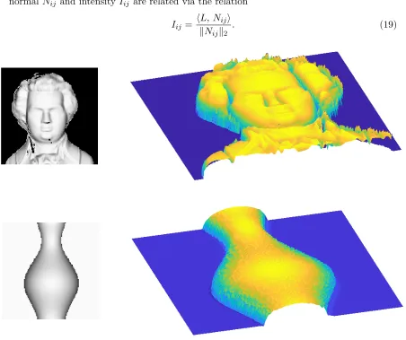
In more detail, suppose that both the object and its 2D image are supported on a rectangular grid of size r×c. We introduce the shorthand notation [r] = {1,2, . . . , r} and [c] = {1,2, . . . , c} for the rows and columns of this grid. For each pair (i, j) ∈ [r]×[c], we let Iij ∈ R denote the observed intensity at location (i, j) in the image, and we let Nij ∈R3 denote the surface normal at the vertex vij : = (xij, yij, zij) of the object. Based on observing the 2-dimensional image, both the intensityIij and co-ordinate pair (xij, yij) are known for each pair (i, j)∈[r]×[c]. The goal of shape from shading is to estimate the unknown coordinate zij, which corresponds to the height of the object at location (i, j). Knowledge of these z-coordinates allows us to generate a 3D representation of the object, as illustrated in Figure 1.
normal Nij and intensity Iij are related via the relation
Iij =
hL, Niji
kNijk2
. (19)
Figure 1. Figure shows 3D shape reconstruction of Mozart (first row) and Vase (second row) from corresponding 2D images. The gray-scale images in the left column are the 2D input images; the two colored images in the right column are the reconstructed 3D shapes. The 3D shapes are constructed by solving the problem (21) using Algorithm 4.
In one standard model (Wang et al., 2014), the surface normal Nij : = (pij, qij,1)> is assumed to be determined by the triplet of vertices (vij, vi+1,j, vi,j+1) via the equations
pij =
(yi,j+1−yi,j)(zi+1,j−zij)−(yi+1,j−yi,j)(zi,j+1−zij) (xi,j+1−xij)(yi+1,j−yij)−(xi+1,j−xij)(yi,j+1−yij) ,
qij =
(xi,j+1−xi,j)(zi+1,j−zij)−(xi+1,j−xi,j)(zi,j+1−zij) (xi,j+1−xij)(yi+1,j−yij)−(xi+1,j−xij)(yi,j+1−yij)
.
Squaring both sides of equation (19) and substituting the expression for surface normalNij yields the polynomial equation
which should be satisfied under the assumed model.
In practice, this equality will not be exactly satisfied, but we can estimate thez-coordinates by solving the following non-convex optimization problem in ther×cmatrixzwith entries
zij |(i, j)∈[r]×[c]}:
min z∈Rr×c
r
X
i=1 c
X
j=1
(1 +p2ij +qij2)Iij2 −(`1pij +`2qij +`3)2
2
| {z }
P(z)
. (21)
Some reconstruction experiments: In order to illustrate the behavior of our method for this problem, we considered two synthetic images for simulated experiments. The first one is a 256×256 image ofMozart (Zhang et al., 1999), and the second one is a 128×128 image ofVase. The 3D shapes were constructed from the 2D images by solving optimization problem (21) using the backtracking gradient descent algorithm 4. The reconstructed sur-faces for Vase and Mozart are provided in Figure 1. We ran 500 iterations of Algorithm 4 for both the images. The runtime forMozart-example was 87 seconds, whereas the runtime forVase-example was 39 seconds. The implementation of Algorithm 4 for Problem (21) is parallelizable; hence, the runtime can be much lower than our runtime with a parallel im-plementation. It is worth mentioning that the polynomial P is a fourth-degree polynomial with dimension r×c; polynomial P is coercive and bounded below by zero. Consequently, we can apply Corollary 2 to the problem (21) which guarantees that average of the squared gradient norm Avg k∇Pk2
2
converges to zero at a rate 1k.
One might also consider applying the CCCP method to this problem. In a recent pa-per, Wang et al. (2014) provided a DC decomposition of the polynomial P using a sum of square (SOS) optimization technique. However, it is crucial to note that the DC decompo-sition of polynomial P obtained from the SOS-optimization method need not be optimal. In order to see this, note that the dimension of the polynomialP is much larger than three. In particular, the variablezij is used in the computation of surface normalsNij, Ni,j−1 and Ni−1,j, hence is related to variables (zi,j+1, zi+1,j, zi−1,j, zi,j−1)—which are again related to the other variables. Ahmadi and Parrilo (2013) showed that SOS techniques for deriving a DC decomposition are sub-optimal for a fourth-degree polynomial when the dimension of the polynomial is greater than three. Consequently, deriving an optimal DC decomposition for the polynomial P will be computationally intensive.
4.2. Robust regression using Tukey’s bi-weight
Next, we turn to the problem of robust regression with Tukey’s bi-weight penalty function. Suppose that we observe pairs (yi, zi)∈R×Rdlinked via the noisy linear model
yi =hzi, µ∗i+εi fori= 1, . . . , n.
vectorµ∗ by computing
min µ∈Rd
1
n n
X
i=1
Ψ yi− hzi, µi
| {z }
= :f(µ)
(22)
where Ψ is a known loss function with some robustness properties. One popular example of the loss function Ψ is Tukey’s bi-weight function, which is given by
Ψ(t) =
(
1−(1−(t/λ)2)3 if|t| ≤λ
1 otherwise, (23)
whereλ >0 is a tuning parameter. Note that Ψ is a smooth function, whence the function f in the objective (22) is also smooth, implying that Algorithm 1 is suitable for the problem.
With this set-up, applying Theorem 1, Theorem 4 and Corollary 3, we obtain the following guarantee:
Corollary 4 Given a random initialization, any bounded sequence {µk}k≥0 obtained by applying Algorithm 1 to the objective (22) has the following properties:
(a) Almost surely with respect to the random initialization, the sequence{µk}k≥0 converges to a point µ¯ such that ∇f(¯µ) = 0 and ∇2f(¯µ)0.
(b) There is a universal constant c1 such that Avgk∇f(µk)k2
≤ c1
k for allk= 1,2, . . ..
We provide the proof in Appendix F.1.
4.3. Smooth function minimization with sparsity constraints
Moving beyond the robust regression problem, we now discuss another interesting prob-lem of minimizing a smooth function subject to sparsity penalty. Consider the following optimization problem
min x∈Rd kxk0≤s
g(x), (24)
where g is a smooth function, the `0-“norm” kxk0 counts the number of non-zero en-tries in the vector x, and s ∈ {1, . . . , d} is a sparsity parameter. The constraint set
x∈Rd| kxk
notation, we have kxk1 ≥Pd
i=d−s+1|x|(i) for all x∈Rd, with equality holding if and only ifx iss–sparse. This fact ensures that
n
x∈Rd:kxk 0 ≤s
o
=
x∈Rd:kxk 1−
d
X
i=d−s+1
|x|(i)≤0 . (25)
Since both of the functionsx7→ kxk1 and x7→Pd
i=d−s+1|x|(i) are convex (Boyd and Van-denberghe, 2004), this level set formulation is a DC constraint. Now using the representa-tion (25), we can rewrite problem (24) as minx∈Rdg(x) such thatkxk1−
Pd
i=d−s+1|x|(i)≤0. For our experiments, it is more convenient to solve the penalized analogue of the last prob-lem, given by
min x∈Rd
g(x) +λ
kxk1−
d
X
i=d−s+1
|x|(i) , (26)
where λ > 0 is a tuning parameter. The optimization problem (26) can be solved using Algorithm 2 with g(x) = g(x), ϕ(x) = λkxk1 and h(x) =λPd
i=d−s+1|x|(i). For the non-smooth componentϕ(x) =λkxk1, there is a closed form expression of the proximal update in Algorithm 2, so that the method is especially efficient in this case.
4.3.1. Best subset selection
A special case of problem (26) arises from best subset selection in linear regression. Suppose that we observe a vector y ∈Rn and a matrix B ∈
Rn×d that are linked via the standard linear model y=Bx∗+ε. Here the vector ε∈ Rn corresponds to additive noise, whereas x∗ ∈ Rd is the unknown regression vector. We wish to estimate the unknown parameter vectorx∗subject to a sparsity constraint, and we do so by solving the following optimization problem:
min x∈Rd kxk0≤s
ky−Bxk22. (27)
Here the non-negative integer s is a tuning parameter that controls maximum number of allowable non-zero entries in the vector x. Following the development leading to the formulation (26), let us consider instead the problem of minimizing the function
f(x) : =ky−Bxk22+λ
kxk1−
d
X
i=d−s+1
|x|(i) . (28)
Note that the function f can be decomposed as a difference of two convex functions as follows:
f(x) =ky−Bxk22+λkxk1
| {z }
convex
−λ
d
X
i=d−s+1
|x|(i)
| {z }
convex
. (29)
Consequently, problem (28) is a DC optimization problem; hence, it is amenable to standard DC optimization techniques like CCCP. We can also apply Algorithm 2 on problem (28) withg(x) =ky−Bxk2
4.3.2. Comparison of Algorithm 2 and CCCP
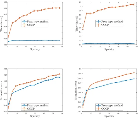
Let us compare the performance of our Algorithm 2 (prox-type method) with the popular convex-concave procedure (CCCP) for minimizing differences of convex functions. We apply both algorithms to the best subset selection problem (28).
Let us reiterate that problem (28) can be written as a difference of two convex functions, and one can apply CCCP update (10) to the decomposition (29). The inner convex opti-mization problem in update (10) is solved by proximal methods for minimizing the sum of a smooth convex function and a`1 regularizer. We also apply Algorithm 2 on problem (28) withg(x) =ky−Bxk2
2,h(x) =λ
Pd
i=d−s+1|x|(i) and ϕ(x) =λkxk1.
Synthetic data generation: We generated the rows of the n×d matrix B from a d -dimensional Gaussian distribution with zero mean and an equicovariance matrix Σ, where Σii= 1 for alli, and Σij = 0.7 for alli6=j. The regression vectorx∗∈Rd(true value) was chosen to be a binary vector with sparsity s (sd). The location of the nonzero entries of the vectorx∗ was chosen uniformly without replacement form the set1, . . . , d .
Performance measures: We use the following two criteria to compare the performance of the prox-type method and CCCP.
(a) Total runtime: Firstly, we compare the algorithms in terms of their total runtime. The runtime was measured in units of seconds.
(b) Estimation error: Secondly, we use average estimation error of the algorithms as a measure of performance. Let us recall that if ¯x ∈ Rd is the estimated value of the unknown regression vectorx∗, then the average estimation error is defined as k¯√x−x∗k2
pk¯xk2 .
Note that the average estimation error used here is invariant under scaling.
Comparison results: Figure 2 shows the performances of the prox-type method and CCCP for synthetic data simulated as above, with problem parameters (n, p) = (190,300) and (n, p) = (380,600) and different choices of sparsity s.
For both the algorithms, the tolerance levelηwas set toη = 10−8, whereas the maximum number of iterations was 1000. Figure 2 suggests that total runtime of the prox-type method is significantly smaller than the runtime of CCCP. Furthermore, the estimation error for the prox-type method is lower compared to CCCP, which possibly suggests that prox-type method is finding better local minima compared to CCCP for the non-convex optimization problem (28). In all our simulations we used same initializations for both the algorithms. The simulation results shown in Figure 2 are average over 100 replications, and we also provide the pointwise error bar in the plots.
4.3.3. Some theoretical guarantees
Interestingly, it turns out that when applied to problem (28), the convergence behavior of Algorithm 2 to a given stationary point ¯x depends on the behavior of a certain convex program defined in terms of ¯x. More precisely, for any point ¯x ∈Rd with|x¯|
(r)>|x¯|(r+1), consider the following convex relaxation of problem (28):
P(¯x) : = min x∈Rd
0 10 20 30 40 50 60 0.02
0.04 0.06 0.08 0.1 0.12 0.14 0.16
0 10 20 30 40 50 60
0.1 0.2 0.3 0.4 0.5 0.6 0.7 0.8 0.9 1 1.1
0 10 20 30 40 50 60
0.02 0.04 0.06 0.08 0.1 0.12 0.14 0.16
0 10 20 30 40 50 60
0.01 0.02 0.03 0.04 0.05 0.06 0.07 0.08 0.09 0.1
Note that|x¯|(r)>|x¯|(r+1)implies the differentiability of the functionh: =λPd
i=d−s+1|x|(i) which ensures that the above problem is well-defined.
Corollary 5 Let xk k≥0 be any bounded sequence obtained by applying Algorithm 2 on problem (28). Suppose there exists a limit pointx¯of the sequencexk k≥0satisfying|x¯|(r)>
|x¯|(r+1), and the convex problem (30) has unique solution. Then the sequence
xk k≥0 converges to the point x, and for all¯ k= 1,2, . . ., we have
Avgk∇f(xk)k2≤ c1
k, and kx k−x¯k
2 ≤cqk, where q ∈(0,1), and (c, c1) are positive constants independent of k.
Comments on problem (30): It can be shown that when the matrixB is of full rank, the objective function in problem (30) is strictly convex, and as a result, the problem (30) has unique solution. In the proof of Corollary 5, we show that the point ¯x is always a minimizer of the convex problem (30), so that the uniqueness assumption implies that ¯x is in fact the unique solution.
4.4. Mixture density estimation
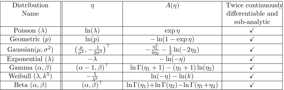
As a final example, we consider the problem of estimating a two-component mixture density, where each of the constituent densities belong to an exponential family. The density of an exponential family (with respect to a fixed base measure, typically counting or Lebesgue) takes the form
p(y;η) =g(y) exp
hη, T(y)i −A(η) . (31)
Here the function T :Y →Rd is a vector of sufficient statistics, whereas the log-partition function
A(η) : = log
Z
Y
g(y) exp{hη, T(y)i}dy
serves to normalize the density. The parameter vector η ∈ Rd determines the choice of density within the family. See Table 1 for some examples of 1-dimensional exponential families of this type. It includes various familiar examples, such as the Gaussian, Poisson and Beta families.
In the problem of mixture density estimation, one is interested in densities of the form
ζ(y;π, η0, η1
| {z }
θ
) =π p(y;η0) + (1−π)p(y;η1), (32)
whereπ ∈(0,1) is an unknown mixing proportion, and (η0, η1) are the unknown parameters of the two underlying densities.
Distribution Name
η A(η) Twice continuously
differentiable and sub-analytic
Poisson (λ) ln(λ) expη X
Geometric (p) ln(p) −ln(1−expη) X
Gaussian(µ, σ2) σµ2,−
1 2σ2
>
−η21
4η2 −
1
2ln(−2η2) X
Exponential (λ) −λ −ln(−η) X
Gamma (α, β) (α−1, β)> ln Γ(η1+ 1)−(η1+ 1) ln(η2) X Weibull (λ, k5) −1
λk ln(−η)−ln(k) X
Beta (α, β) (α, β)> ln Γ(η1)+ln Γ(η2)−ln Γ(η1+η2) X
Table 1. Table showing the natural parameterηand the log-partition functionAfor different densities of exponential family, which are twice continuously differentiable and sub-analytic. In Appendix F.3 we prove the log-partition functionsA mentioned in the above table are sub-analytic.
computing the maximum likelihood estimate (MLE), obtained via minimizing the negative log-likelihood of parameterθgiven by the data. Frequently, a regularized form of the MLE is used, say of the form
min θ
n −
n
X
i=1
log ζ(yi;θ)
| {z }
g(θ)
o
such that η0, η1 ∈Rd,π ∈[0,1], and kη0k2≤R0,kη1k2≤R1.
(33)
Here R0 >0 and R1 >0 are tuning parameters providing upper bound on the `2-norms of the parameters η0 and η1 respectively, often chosen by a data-dependent procedure (such as cross-validation).
By inspection, the objective functiongin problem (33) is non-convex. By standard the-ory on exponential families, the functionAis always infinitely differentiable on its domain, so that the objective functiong is infinitely differentiable on the convex set
X =nθ= (η0, η1, π) | ηj ∈dom(A), π∈[0,1],kηjk2 ≤Rj for j= 0,1
o
.
Consequently, we may apply Algorithm 2 with g(·) = −
n
P
i=1
log ζ(·;yi)
, h≡0 and ϕ(·) =
1X(·) and f = g−h +ϕ. Interestingly, the log-partition function A is sub-analytic for many exponential family densities (see Table 1), which ensures that the function g is also sub-analytic. In Appendix A.3, we show that continuous sub-analytic functions satisfy Assumption KL so that we can apply Theorem 5 to obtain the following:
Corollary 6 Any sequence {θk}k≥0 =ηk0, η1k, πk k≥0 obtained by applying Algorithm 2 to problem (33)satisfies the following properties:
(b) For all k= 1,2, . . ., we have Avg k∇f(θk)k2 ≤ c1
k, where c1 is a universal constant independent of k.
See Appendix F.3 for the proof of this corollary.
5. Discussion
In this paper, we analyzed the behavior of three gradient-based algorithms—namely gradient descent, a proximal method, and an algorithm of the Frank-Wolfe type—for finding critical points of a class of non-convex non-smooth optimization problems. For each of the three algorithms, we provided non-asymptotic bounds on the rate of convergence to a first-order stationary point. We showed that our algorithm can escape strict saddle point for a class of non-smooth functions, thereby generalizing existing results for smooth functions. As a consequence of our theory, we obtained a simplification of the popular CCCP algorithm, and the simplified algorithm retains all the convergence properties of CCCP. Finally, we showed that for a large subclass of functions, which include continuous sub-analytic functions as a special case, we can have a significant improvement in the rate of convergence.
Our work leaves open a number of questions for future research. For instance, it would be interesting to characterize the class of DC-based functions mentioned in problem (2) when the convex function his non-differentiable. Indeed, we then obtain a larger non-class of non-differentiable functions, and we suspect that Theorem 6 can be suitably generalized. Finally, we suspect that the proof techniques used here can be leveraged in order to establish sharper results for other forms of non-convex optimization problems.
Acknowledgments
This work was partially supported by the Office of Naval Research Grant DOD ONR-N00014 and National Science Foundation Grant NSF-DMS-1612948.
Appendix A. Technical background
In this appendix, we collect some technical background on subdifferentials and sub-analytic functions.
A.1. Fr´echet and limiting subdifferential
We first recall the definitions and some useful properties of sub-differentials, which will be useful in subsequent sections.
Definition 1 Let f :Rd 7→ R be a lower semicontinuous function. For any x ∈ dom(f), the Fr´echet subgradient of the functionf at point x is defined as
b
∂f(x) =
(
u
y6=x,y→xlim inf
f(y)−f(x)−
u, y−x ky−xk2
≥0
)
Definition 2 Let f :Rd7→ R be a lower semi-continuous function. For any x∈ dom(f), the limiting subdifferential of the functionf at point x is defined as
∂Lf(x) =
n
u
∃ x
k→x, uk→u with f(xk)→f(x) anduk∈
b
∂f(xk) as k→ ∞o.
Properties: The following properties of Fr´echet and limiting sub-differential are provided in Chapter 8 of Rockafellar and Wets (2009).
(a) For any proper convex function h, we have∂Lh(x) = ∂hb (x) for all x∈ dom(h), and
both quantities agree with the usual subgradient of the convex functionh.
(b) If a functiong is smooth in a neighborhood of a point x, then∂Lf(x) =∇f(x).
(c) Consider a function f of the form f = g+ϕ, where the function g is smooth in a neighborhood of a pointx, and the functionϕis proper convex and finite at the point x. Then the limiting sub-differential of the function f at the point x is given by ∂Lf(x) =∇g(x) +∂ϕ(x).
(d) (Graph continuity:) Consider a sequence xk, uk k≥1 in graph(∂Lf) such that the sequence {(xk, uk, f(xk)}k≥0 converges to a point (x, u, f(x)). Then (x, u) ∈ graph(∂Lf). Recall that graph(∂Lf) : =
(x, u)∈Rd×R |u∈∂Lf(x) . .
A.2. Sub-analytic functions satisfy KL-assumption
In this appendix, we show that continuous sub-analytic functions satisfy the KL-inequality. We also provide examples of functions which are sub-analytic.
Comments on limiting sub-differential: In order to facilitate our discussion, we men-tion some simple facts on limiting subdifferential of a funcmen-tion f, where f is of the form f = g −h (Theorems 1 and 4) or f = g+ϕ−h (Theorems 2 and 5). The following properties are direct consequences of properties of the limiting subdifferential mentioned in Appendix A.1.
• Suppose that the difference functionf =g−hsatisfies parts (a) and (b) of Assumption GR. Then we have
∂L(−f)(x) =∂h(x)− ∇g(x), and moreover
k∇f(x)k2: =k∇g(x)−∂h(x)k2=k∂L(−f)(x)k2
• Suppose that the functionf =g+ϕ−h, where the functionhis locally smooth, and the functionf satisfies Assumption PR part (b). Then∂Lf(x) =∇g(x)− ∇h(x) +∂ϕ(x). Consequently, we have that k∇f(x)k2=k∂Lf(x)k2.
We prove that continuous sub-analytic functions satisfy Assumption KL by exploit-ing results due to Bolte et al. (2007). Let us introduce some notation used in this pa-per. We use mf(x) to denote the `2 distance of the set ∂Lf(x) from zero; concretely, mf(x) := distk·k2 0, ∂Lf(x)
Lemma 1 (Bolte et al. (2007)): Let f : Rd 7→ R∪ {+∞} be a sub-analytic function with closed domain, and assume that f|dom(f) is continuous. Then for any a ∈ dom(f), there exists an exponent θ ∈ [0,1) such that, the function |f−f(a)|m θ
f is bounded above in a neighborhood ofa.
Using Lemma 1, we now argue that sub-analytic functions, under the conditions of Theo-rem 4 or TheoTheo-rem 5, satisfy Assumption KL.
Lemma 2 Any sub-analytic functionf satisfying Assumption GR also satisfies Assumption KL.
Proof First, note that the function f is continuous by Assumption GR; supposef is sub-analytic, then from properties of sub-analytic functions, we have that the function −f is also sub-analytic. Furthermore, the function −f is continuous in the closed domain C — which by Lemma 1 guarantees that, for anya∈ C, there existsθ∈[0,1) such that the ratio
|−f−(−f(a))|θ
m(−f) is bounded above in a neighborhood of the pointa. Since| −f −(−f(a))|= |f −f(a)|, proving satisfiability of Assumption KL reduces to showing that m(−f)(x) is upper bounded by k∇f(x)k2. To this end, note that from the discussion about limiting subdifferential in the paragraph above Lemma 1, we have
k∇f(x)k2 =k∂L(−f)(x)k2 (i)
≥ m(−f)(x), (34)
where step (i) follows from the definition of m(−f)(x). Putting together the pieces, we conclude that any sub-analytic functionf which satisfies Assumption GR, also satisfies As-sumption KL.
Lemma 3 Suppose that, in addition to the conditions on the functions (g, h, ϕ) from The-orem 2, the function f : =g−h+ϕis continuous and sub-analytic in its domain dom(f), and the domain dom(f) is closed. Then the function f satisfies Assumption KL.
Proof Since the function f|dom(f) is continuous and sub-analytic by assumption, from Lemma 1, we have that for any a ∈ dom(f) there exists a θ ∈ [0,1) such that, the ratio
|f−f(a)|θ
mf is bounded above in a neighborhood of the pointa. In order to justify satisfiability of Assumption KL, it suffices to prove that mf(x) is upper bounded by k∇f(x)k2. To this end, note that the function h is locally smooth by assumptions of Theorem 2 part (b). Hence, from the discussion about limiting subdifferential in the paragraph above Lemma 1, we have
k∇f(x)k2 =k∂Lf(x)k2 (i)
≥ mf(x), (35)
A.3. Instances of sub-analytic functions
In Appendix A.2, we proved that continuous sub-analytic functions satisfy Assumption KL, and in those cases,—by Theorems 4 and 5—we have a faster rate of convergence of Algorithms 1 and 2. In this appendix, we provide examples of functions which are sub-analytic. We start by providing definitions of sub-analytic functions following the definition of (Bolte et al., 2007).
A subset S ⊂ Rd is called semi-analytic if each point of
Rd admits a neighborhood V such that the setS∩V has the form
S∩V =∪pi=1∩qj=1
x∈V |hij = 0, gij >0 ,
where the functionshij, gij :V 7→Rare real-analytic.
A set S is calledsub-analytic, if each point ofRd admits a neighborhoodV such that
S∩V =x∈Rd: x, y∈B ,
where B is a bounded semi-analytic subset of Rd×Rm for some m ≥ 1. A function f is called sub-analytic if the graph off, defined by graph(f) : =(x, y)∈Rd×
R:f(x) =y , is sub-analytic.
The class of sub-analytic functions is quite large. In order to motivate the reader, we provide few examples here. The following results can be found in Bolte et al. (2014) and Chapter 6 in the book by Facchinei and Pang (2007).
(a) Any real-valued polynomial or analytic function is sub-analytic.
(b) Any real-valued semi-algebraic or semi-analytic function is sub-analytic.
(c) Indicator function of a semi-algebraic set is sub-analytic.
(d) Sub-analytic functions are closed under finite linear combinations, and the product of two sub-analytic functions is sub-analytic.
(e) Point-wise maximum and minimum of a finite collection of sub-analytic functions are sub-analytic.
(f) Composition rule: If g1 and g2 are two sub-analytic functions with the function g1 being continuous, then the composition function g2◦g1 is sub-analytic. In fact, the class of continuous sub-analytic functions areclosed under algebraic operations.
Appendix B. Proofs related to Algorithm 1
In this appendix, we collect the proofs of various results related to the gradient-based Algorithm 1, including Theorem 1, Corollaries 1 and 3, and Proposition 1.
B.1. Proof of Theorem 1
Lemma 4 Under the conditions of Theorem 1, we have
xk∈int(C) and f(xk+1)≤f(xk)−α
2k∇f(x k)k2
2 for all k= 0,1,2, . . .. (36) See Appendix B.1.1 for the proof of this lemma.
We now prove Theorem 1 using Lemma 4.
Convergence of function values: We first prove that the function value sequence
{f(xk)}k≥0 is convergent. Sincef∗: = min
x∈C f(x) is finite by assumption, andx
k∈int(C) for
all k≥0 by Lemma 4, the sequence{f(xk)}k≥0 is bounded below. For any non-stationary xk, inequality (36) also ensures that f(xk) > f(xk+1); hence, there must exist some scalar
¯
f such that lim k→∞f(x
k) = ¯f.
Stationarity of limit points: Next, we establish that any limit point of the sequence
{xk}k≥0must be stationary. Consider a subsequence{xkj}j≥0ofxk k≥0such thatxkj →x¯, and let {ukj}j≥0 be the associated sequence of subgradients. It suffices to exhibit a sub-gradient ¯u ∈∂h(¯x) such that ∇g(¯x)−u¯= 0. Since the sequence {xkj}
j≥0 converges to ¯x, we must have
k∇f(xkj)k
2 =k∇g(xkj)−ukjk2 →0.
The functiongis continuously differentiable by assumption, and we have∇g(xkj)→ ∇g(¯x). Combining these we find that ukj → ∇g(¯x). Furthermore, by continuity of the function g, we have g(xkj) → g(¯x). Putting together the pieces we have established above that xkj, ukj, g(xkj)→ x,¯ u, g¯ (¯x), where ¯u: =∇g(¯x). Consequently, the graph continuity of limiting-sub-differentials (see Appendix A.1) guarantees that ¯u=∇g(¯x)∈∂h(¯x). Overall, we conclude that ∇f(¯x) : =∇g(x)−u¯= 0, so that ¯x is a stationary point as claimed.
Establishing the bound (3): Finally, we prove the claimed bound (3) on the averaged squared gradient. Recalling that f∗ : = min
x∈C f(x) is finite, we have
f(x0)−f∗ ≥f(x0)−f(xk+1) = k
X
j=0
f(xj)−f(xj+1)
(i)
≥ α
2 k
X
j=0
k∇f(xk)k22
= α(k+ 1) 2 Avg
k∇f(xk)k22,
B.1.1. Proof of Lemma 4
Recall that by assumption, the function g is continuously differentiable and Mg-smooth, and the function h is convex. As a consequence, for any vector xk ∈ C and subgradient uk ∈∂h(xk), we have
g(x)≤g(xk) +h∇g(xk), x−xki+Mg 2 kx−x
kk2
2 (37a)
h(x)≥h(xk) +huk, x−xki. (37b)
Combining inequalities (37a) and (37b) yield
f(x) =g(x)−h(x)≤f(xk) +h∇g(xk)−uk, x−xki+Mg 2 kx−x
kk2
2. (38) Substituting x=xk+1 : =xk−α ∇g(xk)−uk in equation (38) and simplifying yields
f(xk)−f(xk+1)≥ 1
α − Mg
2
kxk+1−xkk2
2=α 1− αMg
2
k∇g(xk)−ukk2 2 (i)
≥ α
2k∇f(x k)k2
2, where inequality (i) follows from the upper bound α ≤ 1
Mg. This proves the second part of the stated lemma. As for the claim that the sequence remains in the interior of the setC, note thatf(xk+1)≤f(xk)≤f(x0), which ensures that xk+1∈ L(f(x0))⊂int(C), as claimed.
B.2. Proof of Corollary 1
The first part of the proof builds on a simple application of Theorem 1 and the definition of effective smoothness constantMf∗. The second part of the proof utilizes a relation between the backtracking step size and the effective smoothness constant. For sake of completeness, we first describe the gradient descent backtracking algorithm.
Algorithm 4 Gradient descent with backtracking
1: Given an initial pointx0 ∈int(C) and parameter β∈(0,1):
2: for k= 0,1,2, . . . do
3: Choose the smallest nonnegative integer ik such that the step size tk: =βik satisfies:
f xk−tk∇f(xk)
≤f(xk)−t
k 2k∇f(x
k)k2. (39)
4: Updatexk+1=xk−tk∇f(xk).
5: end for
Establishing the bound in (5a): For any step size α in the interval 0,M1 f∗