Parsing Techniques A Practical Guide pdf

(1)

PARSING

TECHNIQUES

A Practical Guide

DICK GRUNE CERIEL JACOBS

both of Department of Mathematics and Computer Science Vrije Universiteit, Amsterdam, The Netherlands

Printout by the Authors

(2)

Preface

Parsing (syntactic analysis) is one of the best understood branches of computer science. Parsers are already being used extensively in a number of disciplines: in computer sci-ence (for compiler construction, database interfaces, self-describing data-bases, artifi-cial intelligence), in linguistics (for text analysis, corpora analysis, machine translation, textual analysis of biblical texts), in document preparation and conversion, in typeset-ting chemical formulae and in chromosome recognition, to name a few; they can be used (and perhaps are) in a far larger number of disciplines. It is therefore surprising that there is no book which collects the knowledge about parsing and explains it to the non-specialist. Part of the reason may be that parsing has a name for being “difficult”. In discussing the Amsterdam Compiler Kit and in teaching compiler construction, it has, however, been our experience that seemingly difficult parsing techniques can be explained in simple terms, given the right approach. The present book is the result of these considerations.

This book does not address a strictly uniform audience. On the contrary, while writing this book, we have consistently tried to imagine giving a course on the subject to a diffuse mixture of students and faculty members of assorted faculties, sophisticated laymen, the avid readers of the science supplement of the large newspapers, etc. Such a course was never given; a diverse audience like that would be too uncoordinated to convene at regular intervals, which is why we wrote this book, to be read, studied, perused or consulted wherever or whenever desired.

Addressing such a varied audience has its own difficulties (and rewards). Although no explicit math was used, it could not be avoided that an amount of mathematical thinking should pervade this book. Technical terms pertaining to parsing have of course been explained in the book, but sometimes a term on the fringe of the subject has been used without definition. Any reader who has ever attended a lecture on a non-familiar subject knows the phenomenon. He skips the term, assumes it refers to something reasonable and hopes it will not recur too often. And then there will be pas-sages where the reader will think we are elaborating the obvious (this paragraph may be one such place). The reader may find solace in the fact that he does not have to doo-dle his time away or stare out of the window until the lecturer progresses.

(9)

be hidden behind phrases like:

Let be a mapping V_N →

2(VN∪VT)*

and a homomorphism ...

No knowledge of any particular programming language is required. The book con-tains two or three programs in Pascal, which serve as actualizations only and play a minor role in the explanation. What is required, though, is an understanding of algo-rithmic thinking, especially of recursion. Books like Learning to program by Howard Johnston (Prentice-Hall, 1985) or Programming from first principles by Richard Bornat (Prentice-Hall 1987) provide an adequate background (but supply more detail than required). Pascal was chosen because it is about the only programming language more or less widely available outside computer science environments.

The book features an extensive annotated bibliography. The user of the bibliogra-phy is expected to be more than casually interested in parsing and to possess already a reasonable knowledge of it, either through this book or otherwise. The bibliography as a list serves to open up the more accessible part of the literature on the subject to the reader; the annotations are in terse technical prose and we hope they will be useful as stepping stones to reading the actual articles.

On the subject of applications of parsers, this book is vague. Although we suggest a number of applications in Chapter 1, we lack the expertise to supply details. It is obvious that musical compositions possess a structure which can largely be described by a grammar and thus is amenable to parsing, but we shall have to leave it to the musicologists to implement the idea. It was less obvious to us that behaviour at cor-porate meetings proceeds according to a grammar, but we are told that this is so and that it is a subject of socio-psychological research.

Acknowledgements

We thank the people who helped us in writing this book. Marion de Krieger has retrieved innumerable books and copies of journal articles for us and without her effort the annotated bibliography would be much further from completeness. Ed Keizer has patiently restored peace between us and the pic|tbl|eqn|psfig|troff pipeline, on the many occasions when we abused, overloaded or just plainly misunderstood the latter. Leo van Moergestel has made the hardware do things for us that it would not do for the uninitiated. We also thank Erik Baalbergen, Frans Kaashoek, Erik Groeneveld, Gerco Ballintijn, Jaco Imthorn, and Egon Amada for their critical remarks and contributions. The rose at the end of Chapter 2 is by Arwen Grune. Ilana and Lily Grune typed parts of the text on various occasions.

We thank the Faculteit Wiskunde en Informatica of the Vrije Universiteit for the use of the equipment.

In a wider sense, we extend our thanks to the hundreds of authors who have been so kind as to invent scores of clever and elegant algorithms and techniques for us to exhibit. We hope we have named them all in our bibliography.

Dick Grune Ceriel J.H. Jacobs

(10)

1

Introduction

Parsing is the process of structuring a linear representation in accordance with a given grammar. This definition has been kept abstract on purpose, to allow as wide an interpretation as possible. The “linear representation” may be a sentence, a computer program, a knitting pattern, a sequence of geological strata, a piece of music, actions in ritual behaviour, in short any linear sequence in which the preceding elements in some way restrict†the next element. For some of the examples the grammar is well-known, for some it is an object of research and for some our notion of a grammar is only just beginning to take shape.

For each grammar, there are generally an infinite number of linear representations (“sentences”) that can be structured with it. That is, a finite-size grammar can supply structure to an infinite number of sentences. This is the main strength of the grammar paradigm and indeed the main source of the importance of grammars: they summarize succinctly the structure of an infinite number of objects of a certain class.

There are several reasons to perform this structuring process called parsing. One reason derives from the fact that the obtained structure helps us to process the object further. When we know that a certain segment of a sentence in German is the subject, that information helps in translating the sentence. Once the structure of a document has been brought to the surface, it can be converted more easily.

A second is related to the fact that the grammar in a sense represents our under-standing of the observed sentences: the better a grammar we can give for the move-ments of bees, the deeper our understanding of them is.

A third lies in the completion of missing information that parsers, and especially error-repairing parsers, can provide. Given a reasonable grammar of the language, an error-repairing parser can suggest possible word classes for missing or unknown words on clay tablets.

(11)

1.1 PARSING AS A CRAFT

Parsing is no longer an arcane art; it has not been so since the early 70’s when Aho, Ullman, Knuth and many others put various parsing techniques solidly on their theoret-ical feet. It need not be a mathemattheoret-ical discipline either; the inner workings of a parser can be visualized, understood and modified to fit the application, with not much more than cutting and pasting strings.

There is a considerable difference between a mathematician’s view of the world and a computer-scientist’s. To a mathematician all structures are static: they have always been and will always be; the only time dependence is that we just haven’t discovered them all yet. The computer scientist is concerned with (and fascinated by) the continuous creation, combination, separation and destruction of structures: time is of the essence. In the hands of a mathematician, the Peano axioms create the integers without reference to time, but if a computer scientist uses them to implement integer addition, he finds they describe a very slow process, which is why he will be looking for a more efficient approach. In this respect the computer scientist has more in com-mon with the physicist and the chemist; like these, he cannot do without a solid basis in several branches of applied mathematics, but, like these, he is willing (and often virtu-ally obliged) to take on faith certain theorems handed to him by the mathematician. Without the rigor of mathematics all science would collapse, but not all inhabitants of a building need to know all the spars and girders that keep it upright. Factoring off cer-tain detailed knowledge to specialists reduces the intellectual complexity of a task, which is one of the things computer science is about.

This is the vein in which this book is written: parsing for anybody who has pars-ing to do: the compiler writer, the lpars-inguist, the data-base interface writer, the geologist or musicologist who want to test grammatical descriptions of their respective objects of interest, and so on. We require a good ability to visualize, some programming experi-ence and the willingness and patiexperi-ence to follow non-trivial examples; there is nothing better for understanding a kangaroo than seeing it jump. We treat, of course, the popu-lar parsing techniques, but we will not shun some weird techniques that look as if they are of theoretical interest only: they often offer new insights and a reader might find an application for them.

1.2 THE APPROACH USED

This book addresses the reader at at least three different levels. The interested non-computer scientist can read the book as “the story of grammars and parsing”; he or she can skip the detailed explanations of the algorithms: each algorithm is first explained in general terms. The computer scientist will find much technical detail on a wide array of algorithms. To the expert we offer a systematic bibliography of over 400 entries, which is intended to cover all articles on parsing that have appeared in the readily available journals. Each entry is annotated, providing enough material for the reader to decide if the referred article is worth reading.

(12)

Sec. 1.2] The approach used 15

less widely used methods are almost always described in detail in the original publica-tion, for which see Chapter 13.

1.3 OUTLINE OF THE CONTENTS

Since parsing is concerned with sentences and grammars and since grammars are them-selves fairly complicated objects, ample attention is paid to them in Chapter 2. Chapter 3 discusses the principles behind parsing and gives a classification of parsing methods. In summary, parsing methods can be classified as top-down or bottom-up and as direc-tional or non-direcdirec-tional; the direcdirec-tional methods can be further distinguished into deterministic and non-deterministic. This scheme dictates the contents of the next few chapters. In Chapter 4 we treat non-directional methods, including Unger and CYK. Chapter 5 forms an intermezzo with the treatment of finite-state automata, which are needed in the subsequent chapters. Chapters 6 through 9 are concerned with directional methods. Chapter 6 covers non-deterministic directional top-down parsers (recursive descent, Definite Clause Grammars), Chapter 7 non-deterministic directional bottom-up parsers (Earley). Deterministic methods are treated in Chapters 8 (top-down: LL in various forms) and 9 (bottom-up: LR, etc.). A combined deterministic/non-deterministic method (Tomita) is also described in Chapter 9. That completes the pars-ing methods per se.

Error handling for a selected number of methods is treated in Chapter 10. The comparative survey of parsing methods in Chapter 11 summarizes the properties of the popular and some less popular methods. Chapter 12 contains the full code in Pascal for a parser that will work for any context-free grammar, to lower the threshold for experi-menting.

1.4 THE ANNOTATED BIBLIOGRAPHY

(13)

2

Grammars as a generating device

2.1 LANGUAGES AS INFINITE SETS

In computer science as in everyday parlance, a “grammar” serves to “describe” a “language”. If taken on face value, this correspondence, however, is misleading, since the computer scientist and the naive speaker mean slightly different things by the three terms. To establish our terminology and to demarcate the universe of discourse, we shall examine the above terms, starting with the last one.

2.1.1 Language

To the larger part of mankind, language is first and foremost a means of communica-tion, to be used almost unconsciously, certainly so in the heat of a debate. Communica-tion is brought about by sending messages, through air vibraCommunica-tions or through written symbols. Upon a closer look the language messages (“utterances”) fall apart into sen-tences, which are composed of words, which in turn consist of symbol sequences when written. Languages can differ on all these three levels of composition. The script can be slightly different, as between English and Irish, or very different, as between English and Chinese. Words tend to differ greatly and even in closely related languages people call un cheval or ein Pferd, that which is known to others as a horse. Differences in sentence structure are often underestimated; even the closely related Dutch often has an almost Shakespearean word order: “Ik geloof je niet”, “I believe you not”, and unrelated languages readily come up with constructions like the Hungarian “P nzem van”,

“Money-my is”, where the English say “I have money”.

(14)

Sec. 2.1] Languages as infinite sets 17

The practitioner of formal linguistics, henceforth called the formal-linguist (to dis-tinguish him from the “formal linguist”, the specification of whom is left to the imagi-nation of the reader) again takes an abstracted view of this. A language is a “set” of sentences, and each sentence is a “sequence” of “symbols”; that is all there is: no meaning, no structure, either a sentence belongs to the language or it does not. The only property of a symbol is that it has an identity; in any language there are a certain number of different symbols, the alphabet, and that number must be finite. Just for con-venience we write these symbols as a,b,c . . . , but ✆, ✈, ❑, . . . would do equally well, as long as there are enough symbols. The word sequence means that the symbols in each sentence are in a fixed order and we should not shuffle them. The word set means an unordered collection with all the duplicates removed; a set can be written down by writing the objects in it, surrounded by curly brackets. All this means that to the formal-linguist the following is a language: {a, b, ab, ba}, and so is {a, aa, aaa,

aaaa, . . . } although the latter has notational problems that will be solved later. In

accordance with the correspondence that the computer scientist sees between sentence/word and word/letter, the formal-linguist also calls a sentence a word and he says that “the word ab is in the language {a, b, ab, ba}”.

Now let’s consider the implications of these compact but powerful ideas.

To the computer scientist, a language is a probably infinitely large set of sen-tences, each composed of tokens in such a way that it has structure; the tokens and the structure cooperate to describe the semantics of the sentence, its “meaning” if you will. Both the structure and the semantics are new, that is, were not present in the formal model, and it is his responsibility to provide and manipulate them both. To a computer scientist 3+4*5 is a sentence in the language of “arithmetics on single digits” (“single digits” to avoid having an infinite number of symbols), its structure can be shown, for instance, by inserting parentheses: (3+(4*5)) and its semantics is probably 23.

To the linguist, whose view of languages, it has to be conceded, is much more normal than that of either of the above, a language is an infinite set of possibly interre-lated sentences. Each sentence consists, in a structured fashion, of words which have a meaning in the real world. Structure and words together give the sentence a meaning, which it communicates. Words, again, possess structure and are composed of letters; the letters cooperate with some of the structure to give a meaning to the word. The heavy emphasis on semantics, the relation with the real world and the integration of the two levels sentence/word and word/letters are the domain of the linguist. “The circle

spins furiously” is a sentence, “The circle sleeps red” is nonsense.

The formal-linguist holds his views of language because he wants to study the fundamental properties of languages in their naked beauty; the computer scientist holds his because he wants a clear, well-understood and unambiguous means of describing objects in the computer and of communication with the computer, a most exacting communication partner, quite unlike a human; and the linguist holds his view of language because it gives him a formal tight grip on a seemingly chaotic and perhaps infinitely complex object: natural language.

2.1.2 Grammars

Everyone who has studied a foreign language knows that a grammar is a book of rules and examples which describes and teaches the language. Good grammars make a care-ful distinction between the sentence/word level, which they often call syntax or

(15)

“pour que is followed by the subjunctive, but parce que is not”; grammar contains rules like “the plural of an English noun is formed by appending an -s, except when the word ends in -s, -sh, -o, -ch or -x, in which case -es is appended, or when the word has an irregular plural.”

We skip the computer scientist’s view of a grammar for the moment and proceed immediately to the formal-linguist’s one. His view is at the same time very abstract and quite similar to the above: a grammar is any exact, finite-size, complete description of the language, i.e., of the set of sentences. This is in fact the school grammar, with the fuzziness removed. Although it will be clear that this definition has full generality, it turns out that it is too general, and therefore relatively powerless. It includes descrip-tions like “the set of sentences that could have been written by Chaucer”; platonically speaking this defines a set, but we have no way of creating this set or testing whether a given sentence belongs to this language. This particular example, with its “could have been” does not worry the formal-linguist, but there are examples closer to his home that do. “The longest block of consecutive sevens in the decimal expansion ofπ” describes a language that has at most one word in it (and then that word will consist of sevens only), and as a definition it is exact, finite-size and complete. One bad thing with it, however, is that one cannot find this word; suppose one finds a block of one hundred sevens after billions and billions of digits, there is always a chance that further on there is an even longer block. And another bad thing is that one cannot even know if such a longest block exists at all. It is quite possible that, as one proceeds further and further up the decimal expansion of π, one would find longer and longer stretches of sevens, probably separated by ever-increasing gaps. A comprehensive theory of the decimal expansion ofπmight answer these questions, but no such theory exists.

For these and other reasons, the formal-linguists have abandoned their static, pla-tonic view of a grammar for a more constructive one, that of the generative grammar: a

generative grammar is an exact, fixed-size recipe for constructing the sentences in the

language. This means that, following the recipe, it must be possible to construct each sentence of the language (in a finite number of actions) and no others. This does not mean that, given a sentence, the recipe tells us how to construct that particular sentence, only that it is possible to do so. Such recipes can have several forms, of which some are more convenient than others.

The computer scientist essentially subscribes to the same view, often with the additional requirement that the recipe should imply how a sentence can be constructed.

2.1.3 Problems

The above definition of a language as a possibly infinite set of sequences of symbols, and of a grammar as a finite recipe to generate these sentences, immediately gives rise to two embarrassing questions:

1. How can finite recipes generate enough infinite sets of sentences?

2. If a sentence is just a sequence and has no structure and if the meaning of a sen-tence derives, among other things, from its structure, how can we assess the mean-ing of a sentence?

(16)

2.1.3.1 Infinite sets from finite descriptions

In fact there is nothing wrong with getting a single infinite set from a single finite description: “the set of all positive integers” is a very finite-size description of a defin-itely infinite-size set. Still, there is something disquieting about the idea, so we shall rephrase our question: “Can all languages be described by finite descriptions?”. As the lead-up already suggests, the answer is “No”, but the proof is far from trivial. It is, however, very interesting and famous, and it would be a shame not to present at least an outline of it here.

2.1.3.2 Descriptions can be enumerated

The proof is based on two observations and a trick. The first observation is that descriptions can be listed and given a number. This is done as follows. First, take all descriptions of size one, that is, those of only one letter long, and sort them alphabeti-cally. This is the beginning of our list. Depending on what, exactly, we accept as a description, there may be zero descriptions of size one, or 27 (all letters + space), or 128 (all ASCII characters) or some such; this is immaterial to the discussion which fol-lows.

Second, we take all descriptions of size two, sort them alphabetically to give the second chunk on the list, and so on for lengths 3, 4 and further. This assigns a position on the list to each and every description. Our description “the set of all positive integers”, for instance, is of size 32, not counting the quotation marks. To find its posi-tion on the list, we have to calculate how many descripposi-tions there are with less than 32 characters, say L. We then have to generate all descriptions of size 32, sort them and determine the position of our description in it, say P, and add the two numbers L and P. This will, of course, give a huge number†but it does ensure that the description is on the list, in a well-defined position; see Figure 2.1.

{ descriptions of size 1 { descriptions of size 2 { descriptions of size 3 . . . . .

{

descriptions of size 31 L

. . . .

{

descriptions of size 32

“the set of all positive integers”

P

Figure 2.1 List of all descriptions of length 32 or less

Two things should be pointed out here. The first is that just listing all descriptions alphabetically, without reference to their lengths, would not do: there are already infin-itely many descriptions starting with an “a” and no description starting with a higher

(17)

letter could get a number on the list. The second is that there is no need to actually do all this. It is just a thought experiment that allows us to examine and draw conclusion about the behaviour of a system in a situation which we cannot possibly examine physi-cally.

Also, there will be many nonsensical descriptions on the list; it will turn out that this is immaterial to the argument. The important thing is that all meaningful descrip-tions are on the list, and the above argument ensures that.

2.1.3.3 Languages are infinite bit-strings

We know that words (sentences) in a language are composed of a finite set of symbols; this set is called quite reasonably the alphabet. We will assume that the symbols in the alphabet are ordered. Then the words in the language can be ordered too. We shall indi-cate the alphabet byΣ.

Now the simplest language that uses alphabet Σis that which consists of all words that can be made by combining letters from the alphabet. For the alphabetΣ={a, b} we get the language { , a, b, aa, ab, ba, bb, aaa, . . . }. We shall call this languageΣ*, for reasons to be explained later; for the moment it is just a name.

The set notation Σ* above started with “ { , a,”, a remarkable construction; the first word in the language is the empty word, the word consisting of zero a’s and zero

b’s. There is no reason to exclude it, but, if written down, it may easily get lost, so we

shall write it as ε(epsilon), regardless of the alphabet. So,Σ*={ε, a, b, aa, ab, ba, bb,

aaa, . . . }. In some natural languages, forms of the present tense of the verb “to be”

are the empty word, giving rise to sentences of the form “I student”; Russian and Hebrew are examples of this.

Since the symbols in the alphabet Σ are ordered, we can list the words in the languageΣ*, using the same technique as in the previous section: First all words of size zero, sorted; then all words of size one, sorted; and so on. This is actually the order already used in our set notation forΣ*.

The languageΣ* has the interesting property that all languages using alphabet Σ are subsets of it. That means that, given another possibly less trivial language over Σ, called L, we can go through the list of words inΣ* and put ticks on all words that are in

L. This will cover all words in L, sinceΣ* contains any possible word overΣ.

Suppose our language L is “the set of all words that contain more a’s than b’s”.

L={a, aa, aab, aba, baa, . . . }. The beginning of our list, with ticks, will look as fol-lows:

ε

✔ a

b

✔ aa

ab ba bb

✔ aaa

✔ aab

✔ aba

abb

(18)

bab bba bbb

✔ aaaa

... ...

Given the alphabet with its ordering, the list of blanks and ticks alone is entirely suffi-cient to identify and describe the language. For convenience we write the blank as a 0 and the tick as a 1 as if they were bits in a computer, and we can now write

L=0101000111010001 . . . (and Σ*=1111111111111111 . . . ). It should be noted that this is true for any language, be it a formal language like L, a programming language like Pascal or a natural language like English. In English, the 1’s in the bit-string will be very scarce, since hardly any arbitrary sequence of words is a good English sentence (and hardly any arbitrary sequence of letters is a good English word, depending on whether we address the sentence/word level or the word/letter level).

2.1.3.4 Diagonalization

The previous section attaches the infinite bit-string 0101000111010001... to the description “the set of all the words that contain more a’s than b’s”. In the same vein we can attach such bit-strings to all descriptions; some descriptions may not yield a language, in which case we can attach an arbitrary infinite bit-string to it. Since all descriptions can be put on a single numbered list, we get, for instance, the following picture:

Description Language

Description #1 000000100... Description #2 110010001... Description #3 011011010... Description #4 110011010... Description #5 100000011... Description #6 111011011...

... ...

At the left we have all descriptions, at the right all languages they describe. We now claim that many languages exist that are not on the list of languages above: the above list is far from complete, although the list of descriptions is complete. We shall prove this by using the diagonalization process (“Diagonalverfahren”) of Cantor.

Consider the language C=100110 . . . , which has the property that its n-th bit is unequal to the n-th bit of the language described by Description #n. The first bit of C is a 1, because the first bit for Description #1 is a 0; the second bit of C is a 0, because the second bit for Description #2 is a 1, and so on. C is made by walking the NW to SE diagonal of the language field and copying the opposites of the bits we meet.

The language C cannot be on the list! It cannot be on line 1, since its first bit differs (is made to differ, one should say) from that on line 1, and in general it cannot be on line n, since its n-th bit will differ from that on line n, by definition.

(19)

section of it as follows, . . . . . . . . . . . . . . . . . . . . .. . . ... . . . . . . . . . . . . . . . . . . .. . . . . . . . . . . . . . . . . . . . . ._. . . . . . . . . . . . . . . . . . . . . . .

→

. . . . . . . . . . . . . . . . . . . . .. . . ... . . . . . . . . . . . . . . . . . . .. . . . . . . . . . . . . . . . . . . . . ._. . . . . . . . . . . . . . . . . . . . . . . .

and so does any multiply-broken diagonal. In fact, for each language on the list, there are infinitely many languages not on it; this statement is, however, more graphical than it is exact, and we shall not prove it.

The diagonalization technique is described more formally in most books on theoretical computer science; see e.g., Rayward-Smith [Books 1983, pp. 5-6] or Hop-croft and Ullman [Books 1979, pp 6-9].

2.1.3.5 Conclusions

The above demonstration shows us several things. First, it shows the power of treating languages as formal objects. Although the above outline clearly needs considerable amplification and substantiation to qualify as a proof (for one thing it still has to be clarified why the above explanation, which defines the language C, is not itself on the list of descriptions), it allows us to obtain insight in properties not otherwise assessable. Secondly, it shows that we can only describe a tiny subset (not even a fraction) of all possible languages: there is an infinity of languages out there, forever beyond our reach.

Thirdly, we have proved that, although there are infinitely many descriptions and infinitely many languages, these infinities are not equal to each other and that the latter is larger than the former. These infinities are called ℵ₀ and ℵ₁ by Cantor, and the above is just an adaptation of his proof thatℵ₀<ℵ₁.

2.1.4 Describing a language through a finite recipe

A good way to build a set of objects is to start with a small object and to give rules how to add to it and construct new objects from it. “Two is an even number and the sum of two even numbers is again an even number” effectively generates the set of all even numbers. Formalists will add “...and no other numbers are even”, but we’ll skip that.

Suppose we want to generate the set of all enumerations of names, of the type “Tom, Dick and Harry”, in which all names but the last two are separated by commas. We will not accept “Tom, Dick, Harry” nor “Tom and Dick and Harry”, but we shall not object to duplicates: “Grubb, Grubb and Burrowes”†is all right. Although these are not complete sentences in normal English, we shall still call them sentences since that is what they are in our midget language of name enumerations. A simple-minded recipe would be:

0. Tom is a name, Dick is a name, Harry is a name; 1. a name is a sentence;

(20)

2. a sentence followed by a comma and a name is again a sentence; 3. before finishing, if the sentence ends in “, name”, replace it by

“and name”.

Although this will work for a cooperative reader, there are several things wrong with it. Clause 3 is especially wrought with trouble. For instance, the sentence does not really end in “, name”, it ends in “, Dick” or such, and “name” is just a symbol that stands for a real name; such symbols cannot occur in a real sentence and must in the end be replaced by a real name as given in clause 0. Likewise, the word “sentence” in the recipe is a symbol that stands for all the actual sentences. So there are two kinds of symbols involved here: real symbols, which occur in finished sentences, like “Tom”, “Dick”, a comma and the word “and”; and there are intermediate symbols, like “sen-tence” and “name” that cannot occur in a finished sentence. The first kind corresponds to the words or tokens explained above and the technical term for them is terminal

sym-bols (or terminals for short) while the latter are called non-terminals (a singularly

unin-spired term). To distinguish them, we write terminals in small letters and start non-terminals with a capital.

To stress the generative character of the recipe, we shall replace “X is a Y” by “Y may be replaced by X”: if “tom” is an instance of a Name, then everywhere we have a Name we may narrow it down to “tom”. This gives us:

0. Name may be replaced by “tom” Name may be replaced by “dick” Name may be replaced by “harry” 1. Sentence may be replaced by Name

2. Sentence may be replaced by Sentence, Name

3. “, Name” at the end of a Sentence must be replaced by “and Name” before Name is replaced by any of its replacements

4. a sentence is finished only when it no longer contains non-terminals 5. we start our replacement procedure with Sentence

Clause 0 through 3 describe replacements, but 4 and 5 are different. Clause 4 is not specific to this grammar. It is valid generally and is one of the rules of the game. Clause 5 tells us where to start generating. This name is quite naturally called the start

symbol, and it is required for every grammar.

Still clause 3 looks worrisome; most rules have “may be replaced”, but this one has “must be replaced”, and it refers to the “end of a Sentence”. The rest of the rules work through replacement, but the problem remains how we can use replacement to test for the end of a Sentence. This can be solved by adding an end-marker after it. And if we make the end-marker a non-terminal which cannot be used anywhere except in the required replacement from “, Name” to “and Name”, we automatically enforce the restriction that no sentence is finished unless the replacement test has taken place. For brevity we write -->>instead of “may be replaced by”; since terminal and non-terminal symbols are now identified as technical objects we shall write them in a typewriter-like typeface. The part before the -->>is called the left-hand side, the part after it the

right-hand side. This results in the recipe in Figure 2.2.

(21)

non-0. NNaammee -->> ttoomm N

Naammee -->> ddiicckk N

Naammee -->> hhaarrrryy

1. SSeenntteennccee -->> NNaammee SSeenntteennccee ->-> LLiisstt EEnndd

2. LLiisstt -->> NNaammee L

Liisstt -->> LLiisstt ,, NNaammee

3. ,, NNaammee EEnndd -->> aanndd NNaammee

4. the start symbol is SSeenntteennccee

Figure 2.2 A finite recipe for generating strings in the t, d & h language

terminals left.

2.2 FORMAL GRAMMARS

The above recipe form, based on replacement according to rules, is strong enough to serve as a basis for formal grammars. Similar forms, often called “rewriting systems”, have a long history among mathematicians, but the specific form of Figure 2.2 was first studied extensively by Chomsky [Misc 1959]. His analysis has been the foundation for almost all research and progress in formal languages, parsers and a considerable part of compiler construction and linguistics.

Since formal languages are a branch of mathematics, work in this field is done in a special notation which can be a hurdle to the uninitiated. To allow a small peep into the formal linguist’s kitchen, we shall give the formal definition of a grammar and then explain why it describes a grammar like the one in Figure 2.2. The formalism used is indispensable for correctness proofs, etc., but not for understanding the principles; it is shown here only to give an impression and, perhaps, to bridge a gap.

Definition 2.1: A generative grammar is a 4-tuple (V_N,V_T,R,S) such that (1) V_N and V_T are finite sets of symbols, (2) V_N∩V_T= ∅, (3) R is a set of pairs (P,Q ) such that (3a) P∈(V_N∪V_T)+ and (3b) Q∈(V_N∪V_T)*, and (4) S∈V_N.

A 4-tuple is just an object consisting of 4 identifiable parts; they are the non-terminals, the non-terminals, the rules and the start symbol, in that order; the above defini-tion does not tell this, so this is for the teacher to explain. The set of non-terminals is named V_N and the set of terminals V_T. For our grammar we have:

V_N = {NNaammee,SSeenntteennccee,LLiisstt,EEnndd}

V_T = {ttoomm,ddiicckk,hhaarrrryy,,,,aanndd}

(note the,,in the set of terminal symbols).

The intersection of V_N and V_T (2) must be empty, that is, the non-terminals and the terminals may not have a symbol in common, which is understandable.

R is the set of all rules (3), and P and Q are the left-hand sides and right-hand

sides, respectively. Each P must consist of sequences of one or more non-terminals and terminals and each Q must consist of sequences of zero or more non-terminals and terminals. For our grammar we have:

(22)

Sec. 2.2] Formal grammars 25

(SSeenntteennccee,NNaammee), (SeSenntteennccee,LLiisstt EEnndd),

(LLiisstt,NNaammee), (LLiisstt,LLiisstt ,, NNaammee), (,, NNaammee EEnndd,aanndd NNaammee)}

Note again the two different commas.

The start symbol S must be an element of V_N, that is, it must be a non-terminal:

S =SSeenntteennccee

This concludes our field trip into formal linguistics; the reader can be assured that there is lots and lots more. A good simple introduction is written by R v sz [Books

1985].

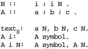
2.2.1 Generating sentences from a formal grammar

The grammar in Figure 2.2 is what is known as a phrase structure grammar for our t,d&h language (often abbreviated to PS grammar). There is a more compact notation, in which several right-hand sides for one and the same left-hand side are grouped together and then separated by vertical bars,||. This bar belongs to the formalism, just as the arrow -->>and can be read “or else”. The right-hand sides separated by vertical bars are also called alternatives. In this more concise form our grammar becomes:

0. NNaammee -->> ttoomm || ddiicckk || hhaarrrryy

1. SSeenntteennccee

S

S -->> NNaammee || LLiisstt EEnndd

2. LLiisstt -->> NNaammee || NNaammee ,, LLiisstt

3. ,, NNaammee EEnndd -->> aanndd NNaammee

where the non-terminal with the subscript

Sis the start symbol. (The subscript S

identi-fies the symbol, not the rule.)

Now let’s generate our initial example from this grammar, using replacement according to the above rules only. We obtain the following successive forms for SSeenn- -tteennccee:

Intermediate form Rule used Explanation

S

Seenntteennccee the start symbol

L

Liisstt EEnndd SSeenntteennccee -->> LLiisstt EEnndd rule 1

N

Naammee ,, LLiisstt EEnndd LLiisstt -->> NNaammee ,, LLiisstt rule 2

N

Naammee ,, NNaammee ,, LLiisstt EEnndd LLiisstt -->> NNaammee ,, LLiisstt rule 2

N

Naammee ,, NNaammee ,, NNaammee EEnndd LLiisstt -->> NNaammee rule 2

N

Naammee ,, NNaammee aanndd NNaammee , N, Naammee EEnndd -->> aanndd NNaammee rule 3

t

toomm ,, ddiicckk aanndd hhaarrrryy rule 0, three times

The intermediate forms are called sentential forms; if a sentential form contains no non-terminals it is called a sentence and belongs to the generated language. The transi-tions from one line to the next are called production steps and the rules are often called

production rules, for obvious reasons.

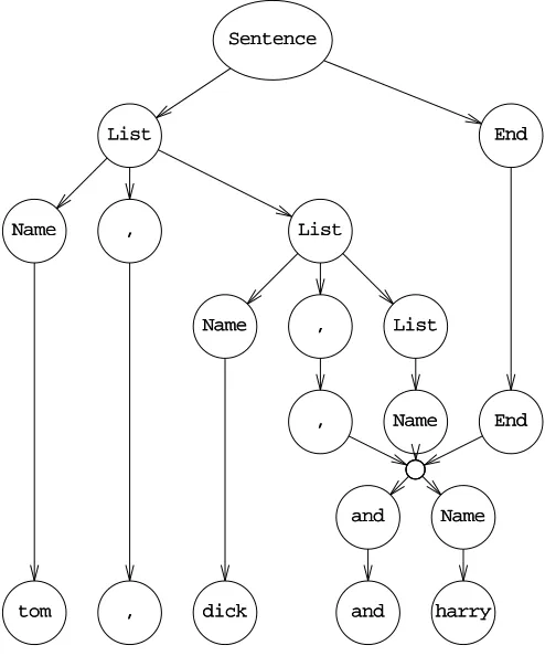
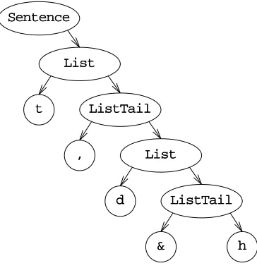
The production process can be made more visual by drawing connective lines between corresponding symbols, as shown in Figure 2.3. Such a picture is called a

pro-duction graph or syntactic graph, because it depicts the syntactic structure (with regard

(23)

SSeenntteennccee

LLiisstt EEnndd

NNaammee ,, LLiisstt

N

Naammee ,, LLiisstt

,

, NNaammee EEnndd

a

anndd NNaammee

[image:23.595.161.408.76.373.2]

ttoomm ,, ddiicckk aanndd hhaarrrryy

Figure 2.3 Production graph for a sentence

fans out downwards, but occasionally we may see starlike constructions, which result from rewriting a group of symbols.

It is patently impossible to have the grammar generate ttoomm,, ddiicckk,, hhaarrrryy, since any attempt to produce more than one name will drag in anEEnnddand the only way to get rid of it again (and get rid of it we must, since it is a non-terminal) is to have it absorbed by rule 3, which will produce the aanndd. We see, to our amazement, that we have succeeded in implementing the notion “must replace” in a system that only uses “may replace”; looking more closely, we see that we have split “must replace” into “may replace” and “must not be a non-terminal”.

Apart from our standard example, the grammar will of course also produce many other sentences; examples are:

hhaarrrryy aanndd ttoomm hhaarrrryy

ttoomm,, ttoomm,, ttoomm,, aanndd ttoomm

and an infinity of others. A determined and foolhardy attempt to generate the incorrect form without theaannddwill lead us to sentential forms like:

ttoomm,, ddiicckk,, hhaarrrryy EEnndd

which are not sentences and to which no production rule applies. Such forms are called

(24)

Sec. 2.2] Formal grammars 27

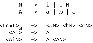
2.2.2 The expressive power of formal grammars

The main property of a formal grammar is that it has production rules, which may be used for rewriting part of the sentential form (= sentence under construction) and a starting symbol which is the mother of all sentential forms. In the production rules we find non-terminals and terminals; finished sentences contain terminals only. That is about it: the rest is up to the creativity of the grammar writer and the sentence pro-ducer.

This is a framework of impressive frugality and the question immediately rises: Is it sufficient? Well, if it isn’t, we don’t have anything more expressive. Strange as it may sound, all other methods known to mankind for generating sets have been proved to be equivalent to or less powerful than a phrase structure grammar. One obvious method for generating a set is, of course, to write a program generating it, but it has been proved that any set that can be generated by a program can be generated by a phrase structure grammar. There are even more arcane methods, but all of them have been proved not to be more expressive. On the other hand there is no proof that no such stronger method can exist. But in view of the fact that many quite different methods all turn out to halt at the same barrier, it is highly unlikely† that a stronger method will ever be found. See, e.g. R v sz [Books 1985, pp 100-102].

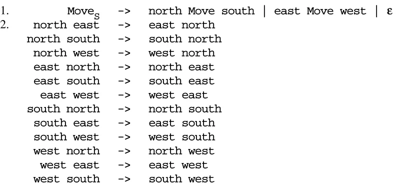
As a further example of the expressive power we shall give a grammar for the movements of a Manhattan turtle. A Manhattan turtle moves in a plane and can only move north, east, south or west in distances of one block. The grammar of Figure 2.4 produces all paths that return to their own starting point.

1. MMoovvee

S

S -->> nnoorrtthh MMoovvee ssoouutthh || eeaasstt MMoovvee wweesstt || εε

2. nnoorrtthh eeaasstt ->-> eeaasstt nnoorrtthh n

noorrtthh ssoouutthh -->> ssoouutthh nnoorrtthh n

noorrtthh wweesstt -->> wweesstt nnoorrtthh e

eaasstt nnoorrtthh -->> nnoorrtthh eeaasstt e

eaasstt ssoouutthh -->> ssoouutthh eeaasstt e

eaasstt wweesstt -->> wweesstt eeaasstt s

soouutthh nnoorrtthh -->> nnoorrtthh ssoouutthh s

soouutthh eeaasstt -->> eeaasstt ssoouutthh s

soouutthh wweesstt -->> wweesstt ssoouutthh w

weesstt nnoorrtthh -->> nnoorrtthh wweesstt w

weesstt eeaasstt -->> eeaasstt wweesstt w

[image:24.595.88.485.386.574.2]

weesstt ssoouutthh -->> ssoouutthh wweesstt

Figure 2.4 Grammar for the movements of a Manhattan turtle

As to rule 2, it should be noted that some authors require at least one of the symbols in the left-hand side to be a non-terminal. This restriction can always be enforced by adding new non-terminals.

The simple round trip nnoorrtthh eeaasstt ssoouutthh wweessttis produced as shown in Fig-ure 2.5 (names abbreviated to their first letter). Note the empty alternative in rule 1

† _{Paul Vit}

ny has pointed out that if scientists call something “highly unlikely” they are still

(25)

(theε), which results in the dying out of the thirdMMin the above production graph.

MM

nn MM ss

e

e MM ww ss

[image:25.595.232.337.105.209.2]

nn ee ss ww

Figure 2.5 How the grammar of Figure 2.4 produces a round trip

2.3 THE CHOMSKY HIERARCHY OF GRAMMARS AND LANGUAGES

The grammars from Figures 2.2 and 2.4 are easy to understand and indeed some simple phrase structure grammars generate very complicated sets. The grammar for any given set is, however, usually far from simple. (We say “The grammar for a given set” although there can be, of course, infinitely many grammars for a set. By the grammar for a set, we mean any grammar that does the job and is not obviously overly compli-cated.) Theory says that if a set can be generated at all (for instance, by a program) it can be generated by a phrase structure grammar, but theory does not say that it will be easy to do so, or that the grammar will be understandable. In this context it is illustra-tive to try to write a grammar for those Manhattan turtle paths in which the turtle is never allowed to the west of its starting point. (Hint: use a special (non-terminal) marker for each block the turtle is located to the east of its starting point).

Apart from the intellectual problems phrase structure grammars pose, they also exhibit fundamental and practical problems. We shall see that no general parsing algo-rithm for them can exist, and all known special parsing algoalgo-rithms are either very inef-ficient or very complex; see Section 3.5.2.

The desire to restrict the unmanageability of phrase structure grammars, while keeping as much of their generative powers as possible, has led to the Chomsky

hierar-chy of grammars. This hierarhierar-chy distinguishes four types of grammars, numbered from

0 to 3; it is useful to include a fifth type, called Type 4 here. Type 0 grammars are the (unrestricted) phrase structure grammars of which we have already seen examples. The other types originate from applying more and more restrictions to the allowed form of the rules in the grammar. Each of these restrictions has far-reaching consequences; the resulting grammars are gradually easier to understand and to manipulate, but are also gradually less powerful. Fortunately, these less powerful types are still very useful, actually more useful even than Type 0. We shall now consider each of the three remaining types in turn, followed by a trivial but useful fourth type.

2.3.1 Type 1 grammars

The characteristic property of a Type 0 grammar is that it may contain rules that transform an arbitrary (non-zero) number of symbols into an arbitrary (possibly zero) number of symbols. Example:

(26)

Sec. 2.3] The Chomsky hierarchy of grammars and languages 29

in which three symbols are replaced by two. By restricting this freedom, we obtain Type 1 grammars. Strangely enough there are two, intuitively completely different definitions of Type 1 grammars, which can be proved to be equivalent.

A grammar is Type 1 monotonic if it contains no rules in which the left-hand side consists of more symbols than the right-hand side. This forbids, for instance, the rule,, NN EE -->> aanndd NN.

A grammar is Type 1 context-sensitive if all of its rules are context-sensitive. A rule is context-sensitive if actually only one (non-terminal) symbol in its left-hand side gets replaced by other symbols, while we find the others back undamaged and in the same order in the right-hand side. Example:

NNaammee CCoommmmaa NNaammee EEnndd -->> NNaammee aanndd NNaammee EEnndd

which tells that the rule

CCoommmmaa -->> aanndd

may be applied if the left context isNNaammeeand the right context isNNaammee EEnndd. The con-texts themselves are not affected. The replacement must be at least one symbol long; this means that context-sensitive grammars are always monotonic; see Section 2.6.

Here is a monotonic grammar for our t,d&h example. In writing monotonic gram-mars one has to be careful never to produce more symbols than will be produced even-tually. We avoid the need to delete the end-marker by incorporating it into the right-most name.

NNaammee -->> ttoomm || ddiicckk || hhaarrrryy S

Seenntteennccee

S

S -->> NNaammee || LLiisstt

LLiisstt -->> EEnnddNNaammee || NNaammee ,, LLiisstt ,

, EEnnddNNaammee ->-> aanndd NNaammee

whereEEnnddNNaammeeis a single symbol.

And here is a context-sensitive grammar for it.

N

Naammee -->> ttoomm || ddiicckk || hhaarrrryy S

Seenntteennccee

SS -->> NNaammee || LLiisstt

L

Liisstt -->> EEnnddNNaammee

|| NNaammee CCoommmmaa LLiisstt C

Coommmmaa EEnnddNNaammee -->> aanndd EEnnddNNaammee context is ... EEnnddNNaammee a

anndd EEnnddNNaammee -->> aanndd NNaammee context is aanndd ... C

Coommmmaa -->> ,,

Note that we need an extra non-terminalCCoommmmaato be able to produce the terminalaanndd

in the correct context.

(27)

languages are known. Although the difference between Type 0 and Type 1 is funda-mental and is not just a whim of Mr. Chomsky, grammars for which the difference matters are too complicated to write down; only their existence can be proved (see e.g., Hopcroft and Ullman [Books 1979, pp. 183-184] or R v sz [Books 1985, p. 98]).

Of course any Type 1 grammar is also a Type 0 grammar, since the class of Type 1 grammars is obtained from the class of Type 0 grammars by applying restrictions. But it would be confusing to call a Type 1 grammar a Type 0 grammar; it would be like calling a cat a mammal: correct but not informative enough. A grammar is named after the smallest class (that is, the highest type number) in which it will still fit.

We saw that our t,d&h language, which was first generated by a Type 0 grammar, could also be generated by a Type 1 grammar. We shall see that there is also a Type 2 and a Type 3 grammar for it, but no Type 4 grammar. We therefore say that the t,d&h language is Type 3 language, after the most restricted (and simple and amenable) gram-mar for it. Some corollaries of this are: A Type n language can be generated by a Type

n grammar or anything stronger, but not by a weaker Type n+1 grammar; and: If a

language is generated by a Type n grammar, that does not necessarily mean that there is no (weaker) Type n+1 grammar for it. The use of a Type 0 grammar for our t,d&h language was a serious case of overkill, just for demonstration purposes.

The standard example of a Type 1 language is the set of words that consist of equal numbers ofaa’s,bb’s andcc’s, in that order:

a a . . . . a

n of them

b b . . . . b

n of them

c c . . . . c

n of them

2.3.1.1 Constructing a Type 1 grammar

For the sake of completeness and to show how one writes a Type 1 grammar if one is clever enough, we shall now derive a grammar for this toy language. Starting with the simplest case, we have the rule

0. SS -->> aabbcc

Having got one instance ofSS, we may want to prepend moreaa’s to the beginning; if we want to remember how many there were, we shall have to append something to the end as well at the same time, and that cannot be a bb or a cc. We shall use a yet unknown symbolQQ. The following rule pre- and postpends:

1. SS -->> aabbcc || aaSSQQ

If we apply this rule, for instance, three times, we get the sentential form

aaaaaabbccQQQQ

Now, to getaaaaaabbbbbbccccccfrom this, eachQQmust be worth onebband onecc, as was to be expected, but we cannot just write

(28)

because that would allow bb’s after the first cc. The above rule would, however, be all right if it were allowed to do replacement only between abband acc; there, the newly insertedbbccwill do no harm:

2. bbQQcc -->> bbbbcccc

Still, we cannot apply this rule since normally theQQ’s are to the right of thecc; this can be remedied by allowing aQQto hop left over acc:

3. ccQQ -->> QQcc

We can now finish our derivation:

aaaaaabbccQQQQ (3 times rule 1)

aaaaaabbQQccQQ (rule 3)

aaaaaabbbbccccQQ (rule 2)

aaaaaabbbbccQQcc (rule 3)

aaaaaabbbbQQcccc (rule 3)

aaaaaabbbbbbcccccc (rule 2)

It should be noted that the above derivation only shows that the grammar will produce the right strings, and the reader will still have to convince himself that it will not gen-erate other and incorrect strings.

S S

SS -->> aabbcc || aaSSQQ

b

bQQcc -->> bbbbcccc c

[image:28.595.196.375.567.698.2]

cQQ -->> QQcc

Figure 2.6 Monotonic grammar for anbncn

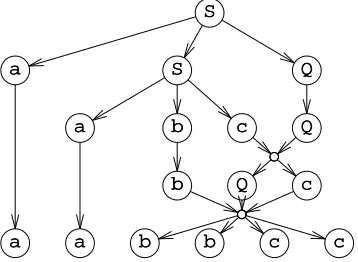
The grammar is summarized in Figure 2.6; since a derivation tree of a3b3c3 is already rather unwieldy, a derivation tree for a2b2c2is given in Figure 2.7. The gram-mar is monotonic and therefore of Type 1; it can be proved that there is no Type 2 grammar for the language.

S S

a

a SS QQ

aa bb cc QQ

bb QQ cc

a

a aa bb bb cc cc

(29)

Type 1 grammars are also called context-sensitive grammars (CS grammars); the latter name is often used even if the grammar is actually monotonic. There are no stan-dard initials for monotonic, but MT may do.

2.3.2 Type 2 grammars

Type 2 grammars are called context-free grammars (CF grammars) and their relation to context-sensitive grammars is as direct as the name suggests. A context-free grammar is like a context-sensitive grammar, except that both the left and the right contexts are required to be absent (empty). As a result, the grammar may contain only rules that have a single non-terminal on their left-hand side. Sample grammar:

0. NNaammee -->> ttoomm || ddiicckk || hhaarrrryy

1. SSeenntteennccee

S

S -->> NNaammee || LLiisstt aanndd NNaammee

2. LLiisstt -->> NNaammee ,, LLiisstt || NNaammee

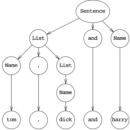
Since there is always only one symbol on the left-hand side, each node in a pro-duction graph has the property that whatever it produces is independent of what its neighbours produce: the productive life of a non-terminal is independent of its context. Starlike forms as we saw in Figures 2.3, 2.5 or 2.7 cannot occur in a context-free pro-duction graph, which consequently has a pure tree-form and is called a propro-duction tree. An example is shown in Figure 2.8.

SSeenntteennccee

L

Liisstt aanndd NNaammee

N

Naammee ,, LLiisstt

NNaammee

t

[image:29.595.180.387.384.591.2]

toomm ,, ddiicckk aanndd hhaarrrryy

Figure 2.8 Production tree for a context-free grammar

Also, since there is only one symbol on the left-hand side, all right-hand sides for a given non-terminal can always be collected in one grammar rule (we have already done that in the above grammar) and then each grammar rule reads like a definition of the left-hand side:

ASSeenntteenncceeis either aNNaammeeor aLLiissttfollowed byaannddfollowed by aNNaammee.

(30)

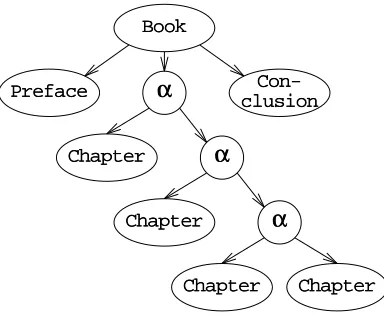
grammars are a very concise way to formulate such interrelationships. An almost trivial example is the composition of a book, as given in Figure 2.9.

B Booookk

SS -->> PPrreeffaaccee CChhaapptteerrSSeeqquueennccee CCoonncclluussiioonn

PPrreeffaaccee ->-> ""PPRREEFFAACCEE"" PPaarraaggrraapphhSSeeqquueennccee C

ChhaapptteerrSSeeqquueennccee -->> CChhaapptteerr || CChhaapptteerr CChhaapptteerrSSeeqquueennccee CChhaapptteerr -->> ""CCHHAAPPTTEERR"" NNuummbbeerr PPaarraaggrraapphhSSeeqquueennccee PPaarraaggrraapphhSSeeqquueennccee -->> PPaarraaggrraapphh || PPaarraaggrraapphh PPaarraaggrraapphhSSeeqquueennccee

P

Paarraaggrraapphh -->> SSeenntteenncceeSSeeqquueennccee SSeenntteenncceeSSeeqquueennccee -->> ...

. ... C

Coonncclluussiioonn -->> ""CCOONNCCLLUUSSIIOONN"" PPaarraaggrraapphhSSeeqquueennccee

Figure 2.9 A simple (and incomplete!) grammar of a book

Of course, this is a context-free description of a book, so one can expect it to also gen-erate a lot of good-looking nonsense like

PPRREEFFAACCEE qqwweerrttyyuuiioopp CCHHAAPPTTEERR VV aassddffgghhjjkkll zzxxccvvbbnnmm,,.. CCHHAAPPTTEERR IIII qqaazzwwssxxeeddccrrffvvttggbb yyhhnnuujjmmiikkoollpp CCOONNCCLLUUSSIIOONN

AAllll ccaattss ssaayy bblleerrtt wwhheenn wwaallkkiinngg tthhrroouugghh wwaallllss..

but at least the result has the right structure. The document preparation and text mark-up language SGML†uses this approach to control the basic structure of documents.

A shorter but less trivial example is the language of all elevator motions that return to the same point (a Manhattan turtle restricted to 5th Avenue would make the same movements)

Z

ZeerrooMMoottiioonn

S

S -->> uupp ZZeerrooMMoottiioonn ddoowwnn ZZeerrooMMoottiioonn

|| ddoowwnn ZZeerrooMMoottiioonn uupp ZZeerrooMMoottiioonn

|| εε

(in which we assume that the elevator shaft is infinitely long; they are, in Manhattan). If we ignore enough detail we can also recognize an underlying context-free struc-ture in the sentences of a natural language, for instance, English:

(31)

S

Seenntteennccee

S

S -->> SSuubbjjeecctt VVeerrbb OObbjjeecctt

S

Suubbjjeecctt -->> NNoouunnPPhhrraassee O

Obbjjeecctt -->> NoNouunnPPhhrraassee

NNoouunnPPhhrraassee -->> ththee QQuuaalliiffiieeddNNoouunn Q

QuuaalliiffiieeddNNoouunn -->> NNoouunn || AAddjjeeccttiivvee QQuuaalliiffiieeddNNoouunn N

Noouunn -->> ccaassttllee || ccaatteerrppiillllaarr || ccaattss

AAddjjeeccttiivvee -->> wweellll--rreeaadd || wwhhiittee || wwiissttffuull || ... V

Veerrbb -->> adadmmiirreess || bbaarrkk || ccrriittiicciizzee || ...

which produces sentences like:

tthhee wweellll--rreeaadd ccaattss ccrriittiicciizzee tthhee wwiissttffuull ccaatteerrppiillllaarr

Since, however, no context is incorporated, it will equally well produce the incorrect

tthhee ccaattss aaddmmiirreess tthhee wwhhiittee wweellll--rreeaadd ccaassttllee

For keeping context we could use a phrase structure grammar (for a simpler language):

S

Seenntteennccee

S

S -->> NNoouunn NNuummbbeerr VVeerrbb

N

Nuummbbeerr -->> SSiinngguullaarr || PPlluurraall

NNoouunn SSiinngguullaarr -->> ccaassttllee SSiinngguullaarr || ccaatteerrppiillllaarr SSiinngguullaarr || ... SSiinngguullaarr VVeerrbb -->> SSiinngguullaarr aaddmmiirreess || ...

S

Siinngguullaarr -->> εε N

Noouunn PPlluurraall -->> cacattss PPlluurraall || ... P

Plluurraall VVeerrbb ->-> PPlluurraall bbaarrkk || PPlluurraall ccrriittiicciizzee || ... P

Plluurraall -->> εε

where the markers SSiinngguullaarr and PPlluurraall control the production of actual English words. Still this grammar allows the cats to bark.... For a better way to handle context, see the section on van Wijngaarden grammars (2.4.1).

The bulk of examples of CF grammars originate from programming languages. Sentences in these languages (that is, programs) have to be processed automatically (that is, by a compiler) and it was soon recognized (around 1958) that this is a lot easier if the language has a well-defined formal grammar. The syntaxes of almost all pro-gramming languages in use today are defined through a formal grammar.†

Some authors (for instance, Chomsky) and some parsing algorithms, require a CF grammar to be monotonic. The only way a CF rule can be non-monotonic is by having an empty right-hand side; such a rule is called anε-rule and a grammar that contains no

such rules is calledε-free. The requirement of beingε-free is not a real restriction, just a nuisance. Any CF grammar can be made ε-free be systematic substitution of the ε -rules (this process will be explained in detail in 4.2.3.1), but this in general does not improve the appearance of the grammar. The issue will be discussed further in Section

Parsing Techniques A Practical Guide pdf

PARSING

TECHNIQUES

A Practical Guide

Table of contents

Preface

1

Introduction

2

Grammars as a generating device

{

{

→