Compact local integrated-RBF approximations for second-order elliptic differential problems

Compact local integrated-RBF approximations for

second-order elliptic differential problems

N. Mai-Duy

_{and T. Tran-Cong}

Computational Engineering and Science Research Centre

Faculty of Engineering and Surveying

University of Southern Queensland, Toowoomba, QLD 4350, Australia

Submitted to

Journal of Computational Physics

, 30-Oct-2010; revised,

21-Feb-2011

AbstractThis paper presents a new compact approximation method for the discretisation of second-order elliptic equations in one and two dimensions. The problem domain, which can be rectangular or non-rectangular, is represented by a Cartesian grid. On stencils, which are three nodal points for one-dimensional problems and nine nodal points for two-dimensional problems, the approximations for the field variable and its derivatives are constructed using integrated radial basis functions (IRBFs). Several pieces of information about the governing differential equation on the stencil are incorporated into the IRBF approximations by means of the constants of integration. Numerical examples indicate that the proposed technique yields a very high rate of convergence with grid refinement.

Keywords: Compact local approximations, high-order approximations, elliptic problems, integrated radial basis functions.

1

Introduction

In the context of finite differences (FDs), approximation schemes can be divided into two categories, namely standard and compact. For standard schemes, on each stencil, derivative values of the field variable u at the central grid point are expressed as linear combinations of nodal values of u only (e.g. [1]). High-order standard approximations require a relatively large stencil. For example, on a one-dimensional (1D) grid, the fourth-order scheme involves a stencil of up to 5 grid points (xj−2, xj−1, xj, xj+1, xj+2). The

centred approximations for the first and second derivatives of the functionuare estimated as

u′

j =

1

h

1

12uj−2− 2

3uj−1 + 2

3uj+1− 1 12uj+2

(1)

u′′

j =

1

h2

− 1

12uj−2+ 4

3uj−1− 5 2uj+

4

3uj+1− 1 12uj+2

where h is the grid size, uj = u(xj), u′j = du(xj)/dx and u′′j = d2u(xj)/dx2. When

large stencils are employed, the sparseness of the system matrix is reduced. In addition, special treatments are needed for grid points close to the boundary as the stencils do not entirely lie within the problem domain. For compact schemes, the FD formulas can be constructed using the Pad´e approximation (e.g. [2,3]). The compact approximations are based on not only nodal function values but also nodal derivative values. One can have high-order approximations on a relatively small stencil. For example, in one dimension, the fourth-order centred compact scheme requires a stencil of 3 grid points only

u′

j−1+ 4u′j +u

′

j+1 = 1

h(−3uj−1+ 3uj+1) (3) u′′_j−1+ 10u

′′

j +u

′′

j+1 = 1

h2 (12uj−1−24uj+ 12uj+1) (4)

Radial basis functions (RBFs), which are radially symmetric about their centres, are known as a powerful tool for approximation of multi-variable data and functions. An RBF is of the formGi(x) =φ(kx−cik), wherexis a field point,ci is a centre andk.kdenotes a

Their solution accuracy is significantly deteriorated.

Many types of RBF, e.g. multiquadric and Gaussian, involve a free shape/width param-eter. Small and large values of the width make these RBFs peaked and flat, respectively. Numerical experiments show that the RBF width has a strong influence on the quality of approximation. This parameter can be used as an alternative to the mesh size in the control of the solution accuracy. Refining the mesh leads to an increase in computational and storage costs, while increasing the RBF width can be implemented without addi-tional costs [14]. For the latter, according to the uncertainty/trade-off principle [15], high accuracy is achieved at the cost of low stability.

Integrated RBFs (IRBFs), in which the highest-order derivatives under consideration are approximated using RBFs and approximate expressions for lower-order derivatives are then obtained through integration, have several advantages over conventional differenti-ated RBFs [16,17]. The purposes of using integration (a smoothing operator) to construct the approximants are (i) to avoid the reduction in convergence rate caused by differentia-tion and (ii) to improve the numerical stability of a discrete soludifferentia-tion. The integradifferentia-tion pro-cess also gives rise to arbitrary constants that serve as additional expansion coefficients, and therefore facilitate the employment of some extra equations. This distinguishing feature of the integral formulation provides effective ways to overcome some difficulties associated with the conventional differential approach, namely (i) the implementation of multiple boundary conditions [18,19,20]; (ii) the imposition of the governing equation on the boundary [21] and (iii) the imposition of high-order continuity of the approximate solution across subdomain interfaces [22]. When IRBFs are implemented in local form, their solution accuracy is also reduced [23].

and Lu are specified at C = (c1,c2,· · · ,cp) and ¯C = (¯c1,c¯2,· · · ,¯cq), respectively. It is

noted that C and ¯C are subsets of X. The RBF approximation for u is constructed as

u(x) =

p

X

i=1

wiφ(kx−cik) + q

X

i=1

λiLφ(kx−¯cik) (5)

wherep≤n;q < n;{wi} p

i=1 and{λi} q

i=1 are sets of unknown coefficients; andL acts onφ which is viewed as a function of the second variable, i.e. ¯c. Approximations to derivatives of u are then obtained through differentiation. Numerical results showed that compact local RBF methods yield superior accuracy and faster convergence than standard local RBF methods.

In this paper, the use of integration to construct compact local RBF schemes is proposed. It will be shown that the constants of integration provide a natural way to include in the IRBF approximations the differential equation at some grid points on the stencil. The paper is organised as follows. A brief review of IRBFs is given in Section 2. In Section 3, the proposed technique is described. Numerical examples are presented in Section 4. Section 5 concludes the paper.

2

Integrated-RBF approximations

Consider a function u(x) with x= (x, y)T_{. The IRBF expressions representing uand its}

derivatives are constructed as follows [17].

In the x direction, the second derivative ofu is first decomposed into RBFs

∂2_u(x)

∂x2 =

N

X

i=1

w_i[x]G[_ix](x) (6)

whereN is the number of RBFs;nw_i[x]oN

i=1the set of weights/coefficients; and

n

G[_ix](x)oN

the set of RBFs. Approximations to the first derivative and the function are then obtained through integration

∂u(x)

∂x =

N

X

i=1

w[_ix]H_i[x](x) +C₁[x](y) (7)

u[x]_{(x) =}

N

X

i=1

w[_ix]H[ix](x) +xC

[x]

1 (y) +C

[x]

2 (y) (8)

where Hi[x](x) =

R

G[ix](x)dx; H

[x]

i (x) =

R

Hi[x](x)dx; and C

[x]

1 (y) and C

[x]

2 (y) are the constants of integration which are univariate functions of the variable y. For points that have the same y coordinate, functions C₁[x](y) andC₂[x](y) on the RHS of (7) and (8) will have the same value.

For the y direction, in the same way, one has

∂2u(x)

∂y2 =

N

X

i=1

w_i[y]G[_iy](x) (9)

∂u(x)

∂y =

N

X

i=1

wi[y]H

[y]

i (x) +C

[y]

1 (x) (10)

u[y]_{(x) =}

N

X

i=1

w_i[y]H[_iy](x) +yC₁[y](x) +C₂[y](x) (11)

It can be seen that there are two approximate values of the functionuat point (x), namely

3

Proposed method

Consider the following elliptic differential problem

Lu=f, x∈Ω (12)

u=r, x∈∂Ω1 (13)

∂u

∂n =s, x∈∂Ω2 (14)

where f, r and s are some prescribed functions; L a second-order linear differential op-erator, e.g. the Laplacian; ∂Ω1 and ∂Ω2 parts of the boundary of the region Ω; and n

the coordinate normal to ∂Ω2. This study is concerned with the development of com-pact local approximations based on IRBFs for the discretisation of (12) in one and two dimensions: (i) Dirichlet and Neumann boundary conditions for 1D domains and 2D do-mains of rectangular shape and (ii) Dirichlet boundary conditions only for 2D dodo-mains of non-rectangular shape.

3.1

1D problems

The domain of interest,a≤x≤b, is discretised by a set of points. The IRBF expressions (6), (7) and (8) reduce to

d2_u(x)

dx2 =

N

X

i=1

wiGi(x) (15)

du(x)

dx =

N

X

i=1

wiHi(x) +C1 (16)

u(x) =

N

X

i=1

wiHi(x) +xC1+C2 (17)

than that of the conventional/differential approach, which allows the addition of two extra equations to the system that represents the conversion of the RBF space into the physical space. In this study, the two extra equations are taken to represent information about (12).

Consider an interior grid point, denoted by x0. On its associated stencil [x1, x2, x3] (x1 < x2 < x3, x0 ≡ x2), we can represent the conversion system as a matrix-vector multiplication             u1 u2 u3 f1 f3             =    H K   

| {z }

C             w1 w2 w3 C1 C2             (18)

where ui =u(xi); fi =f(xi);C is the conversion matrix; andH is defined as

H=      

H1(x1), H2(x1), H3(x1), x1, 1

H1(x2), H2(x2), H3(x2), x2, 1

H1(x3), H2(x3), H3(x3), x3, 1

     

If Lu takes the form, for instance,Lu=d2_u/dx2 _{+u, one will have}

K=

 

 G1(x1) +H1(x1), G2(x1) +H2(x1), G3(x1) +H3(x1), x1, 1

G1(x3) +H1(x3), G2(x3) +H2(x3), G3(x3) +H3(x3), x3, 1

It can be seen that C is an 5×5 matrix. Solving (18) yields             w1 w2 w3 C1 C2            

=C−1

            u1 u2 u3 f1 f3             (19)

which maps the vector of nodal values of the function and the governing equation to the vector of RBF coefficients including the two integration constants.

Approximate expressions for u and its derivatives in the physical space are obtained by substituting (19) into (17), (16) and (15)

u(x) = H1(x), H2(x), H3(x), x,1

C−1



  ub

b

f





 (20)

du(x)

dx = [H1(x), H2(x), H3(x),1,0]C

−1

   ub

b

f

 

 (21)

d2_u(x)

dx2 = [G1(x), G2(x), G3(x),0,0]C

−1

   ub

b

f

 

 (22)

where x1 ≤ x ≤ x3, ub = (u1, u2, u3)T and fb= (f1, f3)T. They can be rewritten in the form

u(x) = 3

X

i=1

ϕi(x)ui+ϕ4(x)f1+ϕ5(x)f3 (23)

du(x)

dx =

3

X

i=1

dϕi(x)

dx ui+

dϕ4(x)

dx f1+

dϕ5(x)

dx f3 (24)

d2_u(x)

dx2 = 3

X

i=1

d2_ϕ

i(x)

dx2 ui+

d2_ϕ

4(x)

dx2 f1+

d2_ϕ5(x)

where {ϕi(x)}5i=1 is the set of IRBFs in the physical space. It can be seen from (23)-(25) that the IRBF approximations for the 3-point stencil scheme are expressed not only in terms of nodal function values but also in terms of nodal derivative values.

3.1.1 Dirichlet boundary conditions

Assume that the values of u are given at x = a and x = b. By collocating (23)-(25) at x = x0 and then substituting the obtained results into (12), we acquire an algebraic equation in terms of nodal variable values for that node. If one applies this task to every interior node and then replaces u(a) and u(b) with given values, this will lead to a determined system of algebraic equations for the unknown values of u at the interior nodes.

3.1.2 Dirichlet and Neumann boundary conditions

Assume that the value of ∂u/∂x andu are given atx=a and x=b, respectively. Unlike the Dirichlet case, the value ofu atx=a is unknown. As a result, one needs to generate one additional algebraic equation for this unknown. The system of algebraic equations thus consists of (N −1) equations for (N −1) unknown values of u, where N is defined here as the number of grid nodes including the two boundary points. We study two ways of implementing the Neumann boundary condition.

Implementation 1: The Neumann boundary condition is incorporated into the IRBF

approximations. The construction of a stencil associated with the grid node next to the boundary pointx=aneeds be modified. The first extra equation in the conversion system (18) is now used to represent the Neumann boundary condition, i.e. f1 =du(a)/dx and the first row of K being [H1(a), H2(a), H3(a),1,0], rather than the governing equation at

equation at the centered point of the stencil and the governing equation at the boundary point x = a, for the final system. The latter is an additional algebraic equation for the value of u at x = a. All (N −1) algebraic equations needed are thus derived from the governing equation only.

Implementation 2: The Neumann boundary condition is imposed in a direct manner. There are no modifications for the construction of a stencil associated with the grid node next to the boundary point x = a. The final system of equations is now added with one extra equation that is generated directly from (21) with x = a. There are thus (N −2) algebraic equations derived from the governing equation and one equation from the Neumann boundary condition.

Implementation 2 is more straightforward to program than Implementation 1.

3.2

2D problems

Two types of the problem domain, rectangular and non-rectangular, are considered. For the former, the compact IRBF approximations on stencils are of similar forms. For the latter, stencils associated with interior nodes close to the boundary may be cut by the boundary, and the nodal points in such stencils are defined in a different way.

3.2.1 Rectangular domain

The problem domain is represented by a Cartesian grid. Consider an interior grid point, denoted by x0. Its associated stencil is defined as



    

x3 x6 x9

x2 x5 x8

x1 x4 x7



where x0 ≡x5. The conversion system for this 9-point stencil is formed as



    

b

u

b

o

b

f



    

=



    

H[x], O H[x], −H[y] K[x]_{, K}[y]



    

| {z }

C

   wb

[x]

b

w[y]

 

whereuband bo are vectors of length 9; wb[x] _{and wb}[y] _{vectors of length 15; O, H}[x] _{and H}[y] matrices of dimensions 9×15; C the conversion matrix;

b

u= (u1,· · · , u9)T

b

w[x]_=w[x]

1 ,· · · , w

[x]

9 , C

[x]

1 (y1), C

[x]

1 (y2), C

[x]

1 (y3), C

[x]

2 (y1), C

[x]

2 (y2), C

[x]

2 (y3)

T

b

w[y]=w[1y],· · · , w

[y]

9 , C

[y]

1 (x1), C

[y]

1 (x4), C

[y]

1 (x7), C

[y]

2 (x1), C

[y]

2 (x4), C

[y]

2 (x7)

T

H[x]=

                         

H[₁x](x1), · · · , H

[x]

9 (x1), x1, 0, 0, 1, 0, 0

H[₁x](x2), · · · , H

[x]

9 (x2), 0, x2, 0, 0, 1, 0

H[₁x](x3), · · · , H

[x]

9 (x3), 0, 0, x3, 0, 0, 1

H[₁x](x4), · · · , H

[x]

9 (x4), x4, 0, 0, 1, 0, 0

H[₁x](x5), · · · , H

[x]

9 (x5), 0, x5, 0, 0, 1, 0

H[₁x](x6), · · · , H

[x]

9 (x6), 0, 0, x6, 0, 0, 1

H[₁x](x7), · · · , H

[x]

9 (x7), x7, 0, 0, 1, 0, 0

H[₁x](x8), · · · , H

[x]

9 (x8), 0, x8, 0, 0, 1, 0

H[₁x](x9), · · · , H

[x]

9 (x9), 0, 0, x9, 0, 0, 1

                         

H[y]=

                         

H[₁y](x1), · · · , H[₉y](x1), y1, 0, 0, 1, 0, 0

H[₁y](x2), · · · , H[₉y](x2), y2, 0, 0, 1, 0, 0

H[₁y](x3), · · · , H[₉y](x3), y3, 0, 0, 1, 0, 0

H[₁y](x4), · · · , H

[y]

9 (x4), 0, y4, 0, 0, 1, 0

H[₁y](x5), · · · , H

[y]

9 (x5), 0, y5, 0, 0, 1, 0

H[₁y](x6), · · · , H[₉y](x6), 0, y6, 0, 0, 1, 0

H[₁y](x7), · · · , H[₉y](x7), 0, 0, y7, 0, 0, 1

H[₁y](x8), · · · , H[₉y](x8), 0, 0, y8, 0, 0, 1

H[₁y](x9), · · · , H[₉y](x9), 0, 0, y9, 0, 0, 1

                          b

u[x]_{(x) is collocated at the grid nodes. In the second sub-system (H}[x]_wb[x] _{= H}[y]_wb[y]_), the approximate nodal values of u obtained from integrating RBFs with respect tox are forced to be identical to those obtained from integrating RBFs with respect to y. The third sub-system, fb= K[x]_wb[x]_+K[y]_wb[y]_{, is used to enforce the governing equation (12)} at some nodes. For illustrative purposes, assume that L is the Laplace operator. We consider the following two cases, which exploit symmetries about the central point x5,

Case 1: Extra equations are used to represent (12) at (x2,x4,x6,x8), i.e.

b

f = (f2, f4, f6, f8)T

K[x]₌

        

G[₁x](x2), · · · , G9[x](x2), 0, 0, 0, 0, 0, 0

G[₁x](x4), · · · , G9[x](x4), 0, 0, 0, 0, 0, 0

G[₁x](x6), · · · , G9[x](x6), 0, 0, 0, 0, 0, 0

G[₁x](x8), · · · , G9[x](x8), 0, 0, 0, 0, 0, 0

        

K[y]₌



       

G[1y](x2), · · · , G

[y]

9 (x2), 0, 0, 0, 0, 0, 0

G[₁y](x4), · · · , G[9y](x4), 0, 0, 0, 0, 0, 0

G[₁y](x6), · · · , G[₉y](x6), 0, 0, 0, 0, 0, 0

G[₁y](x8), · · · , G[₉y](x8), 0, 0, 0, 0, 0, 0



       

Case 2: Extra equations are used to represent (12) at (x1,x3,x7,x9), i.e.

b

f = (f1, f3, f7, f9)T

K[x]₌

        

G[₁x](x1), · · · , G9[x](x1), 0, 0, 0, 0, 0, 0

G[₁x](x3), · · · , G9[x](x3), 0, 0, 0, 0, 0, 0

G[₁x](x7), · · · , G9[x](x7), 0, 0, 0, 0, 0, 0

G[₁x](x9), · · · , G9[x](x9), 0, 0, 0, 0, 0, 0

        

K[y]₌

        

G[1y](x1), · · · , G

[y]

9 (x1), 0, 0, 0, 0, 0, 0

G[₁y](x3), · · · , G[9y](x3), 0, 0, 0, 0, 0, 0

G[₁y](x7), · · · , G[₉y](x7), 0, 0, 0, 0, 0, 0

G[₁y](x9), · · · , G[₉y](x9), 0, 0, 0, 0, 0, 0

        

If Case 2 is implemented, the present approximations will hereafter be named Compact 9-point IRBF (2) or simply Scheme 2.

For Scheme 1 and Scheme 2, the conversion matrix C has more columns than rows. There are an infinite number of solution (wb[x]_,wb[y]₎T _{which exactly satisfy (u,b bo,f}b₎T ₌

C(wb[x]_,wb[y]₎T_{. We apply the SVD technique here to find the unique solution (}

b

w[x]_,wb[y]₎T

which minimises k(w_b[x]_,

b

w[y]₎T_k

2 (minimum norm solution). It is noted that the nodal values of the field variable and the governing equation on the LHS of (26) are satisfied identically. Through (26), the RBF coefficient vectors are computed as

   wb

[x]

b

w[y]

  =C−1

or

b

w[x]_=C−1

[x]

b

u,_bo,fbT (28)

b

w[y]_=C−1

[y]

b

u,bo,fbT (29)

where C−1 _{is the pseudo inverse of the conversion matrix; and C}−1

[x] and C

−1

[y] are the first and last 15 rows ofC−1_{, respectively.}

Using (28) and (29), expressions (7), (6), (10) and (9) atx=x0 become

∂u(x0)

∂x =

h

H₁[x](x0),· · · , H₉[x](x0),0,1,0,0,0,0iC_[−_x1_] bu,o,b fbT (30)

∂2_u(x0)

∂x2 =

h

G[₁x](x0),· · · , G[₉x](x0),0,0,0,0,0,0iC−1

[x]

b

u,bo,fbT (31)

∂u(x0)

∂y =

h

H₁[y](x0),· · ·, H₉[y](x0),0,1,0,0,0,0iC−1

[y]

b

u,bo,fbT (32)

∂2_u(x0)

∂y2 =

h

G[₁y](x0),· · · , G[₉y](x0),0,0,0,0,0,0iC−1

[y]

b

u,o,b fbT (33)

Dirichlet boundary conditions: By collocating (12) at every interior node using (30)-(33) and then replacing the nodal values of u on the boundary with the conditions pre-scribed, one will obtain a determined system of algebraic equations for the unknown values of u at the interior nodes.

Dirichlet and Neumann boundary conditions: Both Implementation 1 and

Imple-mentation 2 for 1D problems are applicable here to handle Neumann boundary conditions.

3.2.2 Non-rectangular domain

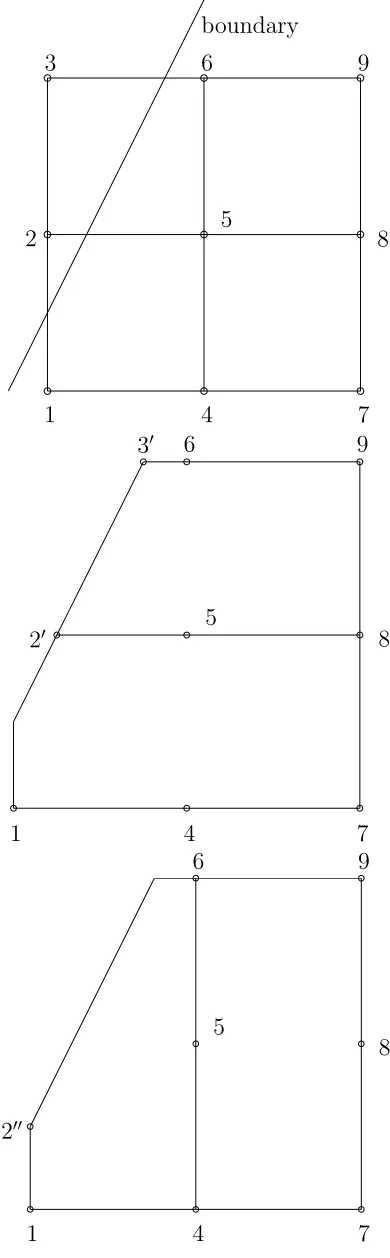
preprocessing here is economical. For interior nodes whose associated stencils lie within the problem domain entirely, the compact IRBF approximations for the field variable and its derivatives have the same forms as in the rectangular-domain case. For interior nodes close to the irregular boundary, the stencils may be cut by the boundary and their shapes become non-rectangular. Consider a typical case as depicted in Figure 1. It can be seen that the boundary points generated by the x and y grid lines do not coincide with the grid nodes. We take the RBF centres as (x1,x2′,x₃′,x₄,x₅,x₆,x₇,x₈,x9) for the

approximation ofu[x]_{(x),∂u(x)/∂xand∂}2_u(x)/∂x2_{, and (x}

1,x2′′,x₄,x₅,x₆,x₇,x₈,x9) for

the approximation of u[y]_{(x), ∂u(x)/∂y and ∂}2_u(x)/∂y2_{. The conversion system is} con-structed as follows. The functionu[x]_{(x) is collocated at the whole set of nodal points used} in the x integration process, i.e. (x1,x2′,x₃′,x₄,x₅,x₆,x₇,x₈,x₉). The functionu[y](x) is

collocated at the boundary points used in they integration process, i.e. (x2′′). The

condi-tionu[x]_{(x) = u}[y]_{(x) is enforced at every interior point, i.e. (x}

1,x4,x5,x6,x7,x8,x9). The

governing equation is collocated at (x4,x6,x8) for Scheme 1 and (x1,x7,x9) for Scheme 2. After solving the conversion system for the RBF coefficient vectors, wb[x] _{and wb}[y]_{, the} approximations are expressed in terms of nodal values of the variable u and the govern-ing equation. The remaingovern-ing steps of the solution procedure are similar to those for the rectangular-domain case. It is noted that this solution procedure is restricted to problems with Dirichlet boundary conditions only.

4

Numerical examples

IRBFs are implemented with the multiquadric (MQ) function

Gi(x) =

p

(x−ci)T(x−ci) +ai (34)

whereci andai are the centre and the width of theith MQ, respectively. For each stencil,

the set of nodal points is taken to be the set of MQ centres. The value of ai is simply

chosen as ai = βhi in which β is a given positive number and hi the smallest distance

between the ith node and its neighbouring grid nodes. We assess the performance of the proposed method through two measures: (i) the relative discrete L2 error defined as

N e(u) =

qPM

i=1(ui−u(ie))2

qPM i=1(u

(e)

i )2

(35)

whereM is the number of nodes over the whole domain and (ii) the convergence rate with respective to grid refinement defined as O(hα_{). The latter is calculated over 2 successive}

grids (point(grid)-wise rate) and also over the whole set of grids used (average rate). The proposed method is validated through the solution of test problems in one and two dimensions.

4.1

Ordinary differential equations (ODEs)

4.1.1 Example 1

Consider the following second-order ODE

d2_u

dx2 =−(2π)

The exact solution to this boundary value problem is chosen to beu(e)_{(x) = sin(2πx).}

Dirichlet boundary conditions: u = 0 is prescribed at x = 0 and x = 1. There are two ways to improve accuracy: (i) the grid is refined (hadaptivity) and (ii) the MQ width is increased (β adaptivity).

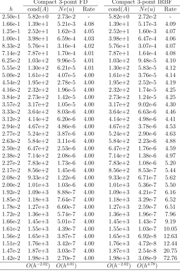
Forhadaptivity, calculations are conducted on sets of uniformly distributed points, from 5 to 71 with an increment of 2. Results concerning the solution accuracy, the convergence rate and the matrix condition by the compact 3-point finite difference (FD) method and the compact 3-point IRBF method are presented in Table 1. Regarding the condition of the system matrix, denoted by cond(A), the two methods have similar values and they grow at the rate O(h−2.02_{). In terms of accuracy, the proposed scheme converges faster.} The point(grid)-wise order of accuracy is about 4 for FDs but can be up to 72.76 for IRBFs. In an average sense, the compact 3-point FD and IRBF solutions converge apparently as

O(h4.01_{) and O(h}4.78_{), respectively. At a grid of 71, the error N e(u) is 2.70×10}−7 _for FDs and 3.08× 10−9 _{for IRBFs. In terms of CPU time, at a grid of 71, the elapsed} times are quite small, i.e. about 0.03s for the proposed method and 0.02s for compact FDM (the computer codes were written using MATLAB and run on a Dell X86-based PC (Intel 3 GHz)). Given a grid size, the CPU time by the proposed method is greater than that by the compact FDM. However, for a prescribed accuracy, the compact FDM requires much more grid nodes than the proposed method. In this regard (accuracy), the proposed method can be more efficient than the compact FDM.

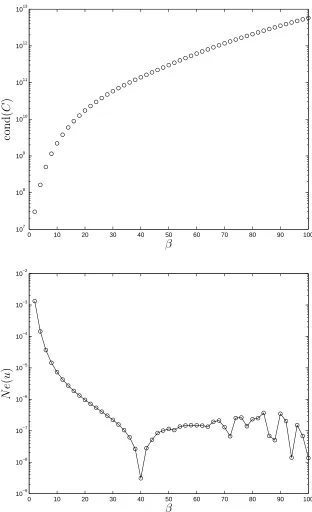
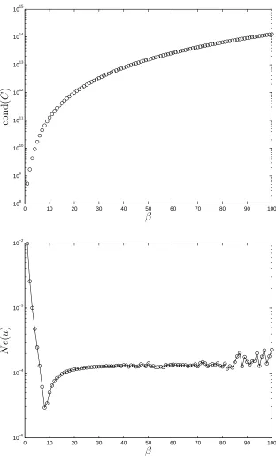
consequence of unbounded error propagation which appears in the solution of highly ill-conditioned system of equations. It appears that the optimal value of β is about 40 and the corresponding matrix condition number (the critical value of the condition number) is 1.39×1011_{. On the other hand, the condition number of the system matrix A does} not change much (about 1.98×103_{) with increasingβ, probably due to the fact that the} matrix A, which is sparse, is constructed in the physical space. It is noted that, from a theoretical point of view, it is still not clear how to choose the optimal value of the MQ width. Unlike global IRBF versions (β = 1 is a preferred value), the present compact IRBF method can work well with a wide range of β. For instance, good accuracy, i.e.

N e(u)<1.e−6, is obtained in a range of 20≤β ≤100.

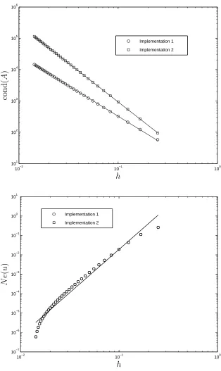
Dirichlet and Neumann boundary conditions: du/dx= 2πandu= 0 are prescribed atx= 0 andx= 1, respectively. Both Implementation 1, in which the Neumann boundary condition is included in the IRBF approximations, and Implementation 2, in which the Neumann boundary condition is imposed in a direct manner, are employed. Figure 3 presents the behaviours of the matrix condition number and the solution accuracy against the grid size. The two implementations produce solutions that have similar degrees of accuracy and converge apparently as O(h4.45_{). This similar behaviour is probably due to} the fact that the two implementations use exactly the same information. In terms of the matrix condition number, Implementation 1 is slightly more stable than Implementation 2. The former (algebraic equations derived from the governing equation only) grows at

O(h−1.94_{), while the latter (algebraic equations derived from the governing equation and} the Neumann boundary condition) at O(h−2.47_).

Non-uniform grids: Such grids are generated here using [24]

xi =

1

2+αsinh

η

1− i−1 N −1

+θ i−1 N −1

(37)

sinh−1(−1/2α) and θ = sinh−1(1/2α). This transformation produces the points that are concentrated nearx= 1/2. The smaller the value of αthe more non-uniform the grid will be. We consider four values α ={2,1,1/2,1/3} employed with β = {40,40,35,30}, respectively (numerical studies indicate that the optimal value of β is reduced as α de-creases). Figure 4 shows results obtained by the present method for Dirichlet boundary conditions. It can be seen that larger values of α (i.e. lower non-uniformity) result in slightly better accuracy and slightly lower matrix condition. It is noted that there is no steep variation in the solution under consideration. Overall, the present method yields quite similar performances over non-uniform grids. The matrix condition number grows slowly (about O(h−2.0_{)), while the solution converges fast (aboutO(h}4.4_)).

Comparison with other RBF methods: Results obtained by the present method are

also compared with those by the global IRBF method and the compact local Hermite RBF method.

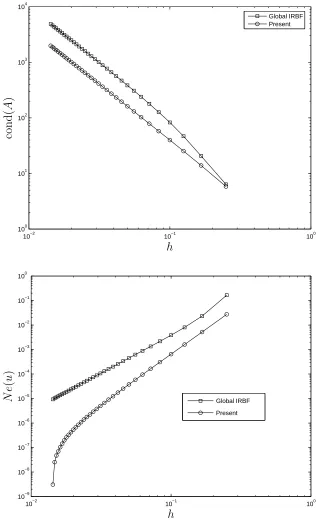
For the global IRBF method [16], the system matrix is non-symmentric and fully popu-lated in contrast to the present scheme, where the system is symmetric and all the nonzero coefficients align themselves along three diagonals. In addition, for stable calculations of global IRBF approximations, one is allowed to use small values of β. Figure 5 shows results obtained by the global IRBF method using β = 1 and by the present method using β = 40. It can be seen that the present method performs much better than the global IRBFN method in terms of both the solution accuracy and the matrix condition.

Following the work of Wright and Fornberg [10], we also implement here a compact 3-point scheme based on Hermite MQ interpolation, which is named compact HRBF. Unlike the method in [10], a direct way of computing the interpolant is employed for compact HRBF. As used in [10], the RBF width is taken here in the form of ε(i.e. ε= 1/a). Decreasingε

the grid sizeh for three values ofεby compact HRBF and IRBF schemes. It can be seen that higher levels of accuracy are obtained with the present IRBF scheme. In addition, at a small valueε = 1.5, IRBF is more stable than HRBF. However, if the Contour-Pad´e algorithm is employed, the latter is able to work for small values of ε and one can thus obtain the optimal solution over a full range ofε, i.e. ε≥0. This point will be illustrated in Section 4.2.2.

4.1.2 Example 2

Find u such that

d2_u

dx2 +

du

dx +u=−exp(−5x) [9979 sin(100x) + 900 cos(100x)], 0≤x≤1 (38)

u(0) = 0 (39)

u(1) = sin(100) exp(−5) (40)

The exact solution can be verified to be

u(e)_{(x) = sin(100x) exp(−5x) (41)}

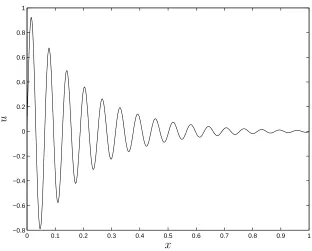
which is highly oscillatory as shown in Figure 7.

It is different from Example 1 that the differential equation here involves three terms and its exact solution has much more complex shape. For the latter, a large number of nodes is required for an accurate simulation.

Figure 8 compares the matrix condition and the solution accuracy for various values ofh

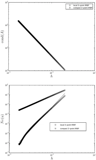
rate of 1.94 by the local IRBF method and of 4.70 with local rates being up to 44.44 by the present compact method. The matrix condition grows as O(h−2.00_{) for both methods.} Results concerning β adaptivity are presented in Figures 9; remarks here are similar to those in Example 1.

4.2

Partial differential equations (PDEs)

4.2.1 Example 1

The PDE under consideration here is taken in the form

∂2_u

∂x2 +

∂2_u

∂y2 =−2π

2_{sin(πx) sin(πy) (42)}

The domain of interest is a unit square 0 ≤ x, y ≤ 1. The exact solution to (42) is

u(e)_{(x, y) = sin(πx) sin(πy). The local 9-point IRBF method and two schemes of the} present compact 9-point IRBF method are employed.

Dirichlet boundary conditions: u= 0 is specified on the entire boundary.

and run on a Dell X86-based PC (Intel 3 GHz)).

To study the effect of β adaptivity, a wide range ofβ is employed. Figure 11 plotsN e(u) against β. Both schemes can work at large values of β. The error N e(u) is a decreasing function of β up to the value of 60 for Scheme 1 and 25 for Scheme 2.

Scheme 1 outperforms Scheme 2 regarding accuracy for both h and β adaptivities.

Dirichlet and Neumann boundary conditions: Dirichlet boundary conditions are

prescribed on x = 0 and x = 1 with 0 ≤ y ≤ 1, while Neumann boundary conditions are specified on y = 0 and y = 1 with 0 < x < 1. As shown in Section 4.1.1, the two implementations of a Neumann boundary condition produce similar degrees of accuracy. We employ Implementation 2 here. The matrix condition and solution accuracy by Scheme 1 and Scheme 2 are shown in Figure 12. Scheme 1 yields slightly larger condition numbers but much more accurate results than Scheme 2. The compact local IRBFN solution converges as O(h3.90_{) for Scheme 1 and O(h}4.04_{) for Scheme 2. It should be pointed out} that these rates are as high as those for the case of Dirichlet boundary conditions only.

4.2.2 Example 2

Example 2 is similar to Example 1, except that the exact solution now takes the form

For RBF-FD and RBF-HFD, the Contour-Pad´e algorithm is employed, which allows stable calculations of the interpolant for a full range of ε, i.e. ε ≥ 0. In contrast, by using the direct way of computing the IRBF interpolant (i.e. directly solving (26)), Scheme 1 is limited to large values of ε.

Figure 13 displays the solution accuracy against the grid size by RBF-FD, RBF-HFD and Scheme 1 for several values of ε. It can be seen that, for large values of ε, i.e. 2.0 and 1.6, Scheme 1 is more accurate than RBF-FD and RBF-HFD. Decreasing ε can improve accuracy significantly. As shown in [25], the highest accuracy is often found for values ofε

that cause the direct computation of the interpolant to suffer from severe ill-conditioning. Numerical experiments showed that the optimal value ofε is about 1.6 for RBF-FD ([10], Table 3), 0.85 for RBF-HFD ([10], Table 4) and 1.6 for Scheme 1. The first two are found over a full range of ε, while the last one is found overε−values that make the direct way of computing the interpolant stable. RBF-HFD yields better accuracy than Scheme 1 for the optimal value of ε. It is expected that overcoming a severely ill-conditioned problem of Scheme 1 will extend its range of ε and thus improve its highest accuracy.

4.2.3 Example 3

Consider the following PDE

∂2_u

∂x2 +

∂2_u

∂y2 = 4(1−π

2_{) sin(2πx) sinh(2y) + 16(1−π}2_{) cosh(4x) cos(4πy) (43)}

condition and the solution accuracy against the grid size for several values ofβ.

In the case of curved boundary, there may be interior points that are very close the boundary. Since their associated compact stencils employ the boundary nodes as the RBF centres, there are sudden changes in the distance between the nodal points in these stencils. They can be seen to be a random function of grid density. Figure 15 shows that the matrix condition behaviour has some fluctuation. For Scheme 1, the matrix condition grows as O(h−2.85_{), O(h}−2.85_{) and O(h}−2.85_{) for the three values of β. For Scheme 2, it} grows as O(h−2.79_{), O(h}−2.79_{) and O(h}−2.79_{) for the three values of β. These rates are} higher than those in the rectangular-domain case.

In spite of having some fluctuation in the matrix condition behaviour, the compact local IRBF solution still converges very fast and quite smoothly (Figure 15). Using

β = (20,30,40), the rates are O(h4.03_{), O(h}4.02_{) O(h}4.02_{) for Scheme 1 and O(h}3.84_),

O(h3.83_{) O(h}3.83_{) for Scheme 2.}

Each scheme of the proposed method has thus similar performances in terms of the matrix condition and the solution accuracy for different values of β, which makes the choice of

β easy in practice. Like in the rectangular case, Scheme 1 outperforms Scheme 2. The former is recommended for use.

Implementation notes:

In the 2D case, the present discretisation formulations are based on Cartesian grids. Numerical results indicate that high rates of convergence are obtained for both rectan-gular and non-rectanrectan-gular domains. The present method is simpler in implementation (no fourth-order derivatives involved) but less flexible in discretisation (structured grids required) than the RBF-HFD method.

As shown in Figures 10 and 12, the way of incorporating the governing PDE into the approximations has a strong influence on the solution accuracy. Our various numerical studies of the number and location of additional nodes used for the PDE on the stencil indicate that Scheme 1 yields the most accurate results.

5

Conclusions

In this paper, a new compact local approximation method is proposed for the discreti-sation of second-order elliptic problems defined on rectangular and non-rectangular do-mains. The preprocessing is economical as Cartesian grids are used to represent the problem domain. The present IRBF approximations are constructed locally and each lo-cal construction has its own set of extra coefficients (a set of integration constants) which are exploited to impose the governing equation. They utilise more information about the governing equation than standard IRBF approximations, leading to a significant im-provement in accuracy. This study further demonstrates the usefulness of the integration constants. The proposed method is validated successfully through a series of test prob-lems in one and two dimensions. Very accurate results are obtained using relatively coarse grids.

Analytic forms of the integrated MQ basis functions used are given below

H_i[x](x) = (x−x

†

i)

2 Q+

S[x] 2 R

[x] ₍₄₄₎

H_i[y](x) = (y−y

†

i)

2 Q+

S[y] 2 R

[y] ₍₄₅₎

H[_ix](x) = (x−x

†

i)2

6 −

S[x] 3

!

Q+ S

[x]_(x−x†

i)

2 R

[x] ₍₄₆₎

H[_iy](x) = (y−y

†

i)2

6 −

S[y] 3

!

Q+ S

[y]_(y−y†

i)

2 R

[y] ₍₄₇₎

where x= (x, y)T_;c

i = (x†i, y

†

i)T; r =kx−cik;

Q=

q

r2_+a2

i (48)

R[x]_{= ln(x−x}†

i) +Q

(49)

R[y]_{= ln(y−y}†

i) +Q

(50)

S[x] _=r2_−(x−x†

i)

2_+a2

i (51)

S[y]_=r2_−(y−y†

i)

2_+a2

i (52)

Acknowledgements

This work is supported by the Australian Research Council. The authors would like to thanks the referees for their helpful comments.

References

1. P.J. Roache, Fundamentals of Computational Fluid Dynamics, Hermosa Publishers, Albuquerque, 1998.

3. S.K. Lele, Compact finite difference schemes with spectral-like resolution, Journal of Computational Physics 103(1) (1992) 16–42.

4. G.E. Fasshauer, Meshfree Approximation Methods With Matlab (Interdisciplinary Mathematical Sciences - Vol. 6), World Scientific Publishers, Singapore, 2007.

5. E.J. Kansa, Multiquadrics- A scattered data approximation scheme with applica-tions to computational fluid-dynamics-II. Soluapplica-tions to parabolic, hyperbolic and el-liptic partial differential equations, Computers and Mathematics with Applications 19(8/9) (1990) 147–161.

6. C.K. Lee, X. Liu, S.C. Fan, Local multiquadric approximation for solving boundary value problems, Computational Mechanics 30(5–6) (2003) 396–409.

7. C. Shu, H. Ding, K.S. Yeo, Local radial basis function-based differential quadrature method and its application to solve two-dimensional incompressible Navier-Stokes equations, Computer Methods in Applied Mechanics and Engineering 192 (2003) 941–954.

8. A.I. Tolstykh, D.A. Shirobokov, On using radial basis functions in a finite differ-ence mode with applications to elasticity problems, Computational Mechanics 33(1) (2003) 68–79.

9. A.I. Tolstykh, D.A. Shirobokov, Using radial basis functions in a “finite difference mode”, CMES: Computer Modeling in Engineering & Sciences 7(2) (2005) 207–222.

10. G.B. Wright, B. Fornberg, Scattered node compact finite difference-type formulas generated from radial basis functions, Journal of Computational Physics 212(1) (2006) 99–123.

12. Y.V.S.S. Sanyasiraju, G. Chandhini, Local radial basis function based gridfree scheme for unsteady incompressible viscous flows, Journal of Computational Physics 227(20) (2008) 8922–8948.

13. R. Vertnik, B. Sarler, Solution of incompressible turbulent flow by a mesh-free method, CMES: Computer Modeling in Engineering & Sciences 44(1) (2009) 65–96.

14. A.H.-D. Cheng, M.A. Golberg, E.J. Kansa, G. Zammito, Exponential convergence and H-c multiquadric collocation method for partial differential equations, Numer-ical Methods for Partial Differential Equations 19 (2003) 571–594.

15. R. Schaback, Error estimates and condition numbers for radial basis function inter-polation, Advances in Computational Mathematics 3 (1995) 251–264.

16. N. Mai-Duy, T. Tran-Cong, Numerical solution of differential equations using mul-tiquadric radial basis function networks, Neural Networks 14(2) (2001) 185–199.

17. N. Mai-Duy, T. Tran-Cong, Approximation of function and its derivatives using radial basis function networks, Applied Mathematical Modelling 27 (2003) 197–220.

18. N. Mai-Duy, Solving high order ordinary differential equations with radial basis function networks, International Journal for Numerical Methods in Engineering 62 (2005) 824–852.

19. N. Mai-Duy, R.I. Tanner, Solving high order partial differential equations with in-direct radial basis function networks, International Journal for Numerical Methods in Engineering 63 (2005) 1636–1654.

20. N. Mai-Duy, T. Tran-Cong, Solving biharmonic problems with scattered-point dis-cretisation using indirect radial-basis-function networks, Engineering Analysis with Boundary Elements 30(2) (2006) 77–87.

for Heat & Fluid Flow 17(2) (2007) 165–186.

22. N. Mai-Duy, T. Tran-Cong, A multidomain integrated radial basis function col-location method for elliptic problems, Numerical Methods for Partial Differential Equations 24 (2008) 1301–1320.

23. N. Mai-Duy, T. Tran-Cong, A Cartesian-grid discretisation scheme based on local integrated RBFNs for two-dimensional elliptic problems, CMES: Computer Model-ing in EngineerModel-ing & Sciences 51(3) (2009) 213–238.

24. D. Tavella, C. Randall, Pricing Financial Instruments: The Finite Difference Method, John Wiley & Sons, New York, 2000.

Table 1: ODE, Example 1, Dirichlet boundary conditions, N = (5,7,· · · ,71): Condition numbers of the system and relative L2 errors of the approximate solution u for various values ofhby the compact 3-point finite-difference method and the compact 3-point IRBF method (β = 40).

Compact 3-point FD Compact 3-point IRBF

h cond(A) N e(u) Rate cond(A) N e(u) Rate 2.50e-1 5.82e+0 2.73e-2 - 5.82e+0 2.72e-2 -1.66e-1 1.39e+1 5.21e-3 4.08 1.39e+1 5.17e-3 4.09 1.25e-1 2.52e+1 1.62e-3 4.05 2.52e+1 1.60e-3 4.07 1.00e-1 3.98e+1 6.59e-4 4.03 3.98e+1 6.47e-4 4.06 8.33e-2 5.76e+1 3.16e-4 4.02 5.76e+1 3.07e-4 4.07 7.14e-2 7.87e+1 1.70e-4 4.01 7.87e+1 1.64e-4 4.08 6.25e-2 1.03e+2 9.96e-5 4.01 1.03e+2 9.48e-5 4.10 5.55e-2 1.30e+2 6.21e-5 4.01 1.30e+2 5.83e-5 4.12 5.00e-2 1.61e+2 4.07e-5 4.00 1.61e+2 3.76e-5 4.14 4.54e-2 1.95e+2 2.78e-5 4.00 1.95e+2 2.52e-5 4.19 4.16e-2 2.32e+2 1.96e-5 4.00 2.32e+2 1.74e-5 4.25 3.84e-2 2.73e+2 1.42e-5 4.00 2.73e+2 1.24e-5 4.25 3.57e-2 3.17e+2 1.05e-5 4.00 3.17e+2 9.02e-6 4.30 3.33e-2 3.64e+2 8.03e-6 4.00 3.64e+2 6.63e-6 4.46 3.12e-2 4.14e+2 6.20e-6 4.00 4.14e+2 4.98e-6 4.41 2.94e-2 4.67e+2 4.86e-6 4.00 4.67e+2 3.78e-6 4.53 2.77e-2 5.24e+2 3.87e-6 4.00 5.24e+2 2.90e-6 4.63 2.63e-2 5.84e+2 3.11e-6 4.00 5.84e+2 2.23e-6 4.88 2.50e-2 6.47e+2 2.53e-6 4.00 6.47e+2 1.76e-6 4.59 2.38e-2 7.14e+2 2.08e-6 4.00 7.14e+2 1.38e-6 4.97 2.27e-2 7.83e+2 1.73e-6 4.00 7.83e+2 1.08e-6 5.20 2.17e-2 8.56e+2 1.45e-6 4.00 8.56e+2 8.53e-7 5.44 2.08e-2 9.33e+2 1.22e-6 4.00 9.33e+2 6.71e-7 5.62 2.00e-2 1.01e+3 1.03e-6 4.00 1.01e+3 5.36e-7 5.50 1.92e-2 1.09e+3 8.88e-7 4.00 1.09e+3 4.21e-7 6.16 1.85e-2 1.18e+3 7.64e-7 4.00 1.18e+3 3.29e-7 6.52 1.78e-2 1.27e+3 6.60e-7 4.00 1.27e+3 2.59e-7 6.51 1.72e-2 1.36e+3 5.74e-7 4.00 1.36e+3 1.96e-7 7.96 1.66e-2 1.45e+3 5.01e-7 4.00 1.45e+3 1.43e-7 9.19 1.61e-2 1.55e+3 4.39e-7 4.00 1.55e+3 1.03e-7 10.05 1.56e-2 1.65e+3 3.87e-7 4.00 1.65e+3 6.92e-8 12.63 1.51e-2 1.76e+3 3.42e-7 4.00 1.76e+3 4.72e-8 12.44 1.47e-2 1.87e+3 3.03e-7 4.00 1.87e+3 2.54e-8 20.75 1.42e-2 1.98e+3 2.70e-7 4.00 1.98e+3 3.08e-9 72.76

boundary

1 2

3

4 5 6

7 8 9

1 2′

3′

4 5 6

7 8 9

1 2′′

4 5 6

7 8 9

0 10 20 30 40 50 60 70 80 90 100 107

108 109 1010 1011 1012 1013

β

co

n

d

(

C

)

0 10 20 30 40 50 60 70 80 90 100 10−9

10−8 10−7 10−6 10−5 10−4 10−3 10−2

β

N

e

(

u

)

10−2 10−1 100 101

102 103 104 105 106

Implementation 1 Implementation 2

h

co

n

d

(

A

)

10−2 10−1 100

10−7 10−6 10−5 10−4 10−3 10−2 10−1 100 101

Implementation 1 Implementation 2

h

N

e

(

u

)

10−2 10−1 100 100

101 102 103 104

α=2

α=1

α=1/2

α=1/3

h

co

n

d

(

A

)

10−2 10−1 100

10−8 10−7 10−6 10−5 10−4 10−3 10−2 10−1

α=2

α=1

α=1/2

α=1/3

h

N

e

(

u

)

10−2 10−1 100 100

101 102 103 104

Global IRBF Present

h

co

n

d

(

A

)

10−2 10−1 100

10−9 10−8 10−7 10−6 10−5 10−4 10−3 10−2 10−1 100

Global IRBF Present

h

N

e

(

u

)

ε= 4.5

10−2 10−1 100

10−6 10−5 10−4 10−3 10−2 10−1 100

HRBF IRBF

h

N

e

(

u

)

ε= 3.0

10−2 ₁₀−1 ₁₀0

10−7 10−6 10−5 10−4 10−3 10−2 10−1

HRBF IRBF

h

N

e

(

u

)

ε= 1.5

10−2 10−1 100

10−8 10−7 10−6 10−5 10−4 10−3 10−2 10−1

HRBF IRBF

h

N

e

(

u

0 0.1 0.2 0.3 0.4 0.5 0.6 0.7 0.8 0.9 1 −0.8

−0.6 −0.4 −0.2 0 0.2 0.4 0.6 0.8 1

x

u

10−3 10−2 10−1 103

104 105 106

local 3−point IRBF compact 3−point IRBF

h

co

n

d

(

A

)

10−3 10−2 10−1

10−7 10−6 10−5 10−4 10−3 10−2 10−1 100

local 3−point IRBF compact 3−point IRBF

h

N

e

(

u

)

Figure 8: ODE, Example 2, Dirichlet boundary conditions, N = (51,53,55,· · · ,591),

0 10 20 30 40 50 60 70 80 90 100 108

109 1010 1011 1012 1013 1014 1015

β

co

n

d

(

C

)

0 10 20 30 40 50 60 70 80 90 100 10−5

10−4 10−3 10−2

β

N

e

(

u

)

10−2 10−1 100 100

101 102 103

local 9−point IRBF compact 9−point IRBF (1) compact 9−point IRBF (2)

h

co

n

d

(

A

)

10−2 10−1 100

10−7 10−6 10−5 10−4 10−3 10−2 10−1

local 9−point IRBF compact 9−point IRBF (1) compact 9−point IRBF (2)

h

N

e

(

u

)

Figure 10: PDE, Example 1, rectangular domain, (5×5,7×7,· · · ,37×37), β = 45:

0 10 20 30 40 50 60 70 80 90 100 10−8

10−7 10−6 10−5 10−4 10−3 10−2

compact 9−point IRBF (1) compact 9−point IRBF (2)

β

N

e

(

u

)

10−2 10−1 100 101

102 103 104

compact 9−point IRBF (1) compact 9−point IRBF (2)

h

co

n

d

(

A

)

(b) Matrix condition

10−2 10−1 100

10−7 10−6 10−5 10−4 10−3 10−2 10−1 100

compact 9−point IRBF (1) compact 9−point IRBF (2)

h

N

e

(

u

)

(a) Solution accuracy

ε= 2.0

10−2 10−1 100

10−7 10−6 10−5 10−4 10−3 10−2 10−1 Present RBF−FD RBF−HFD h M ax n or m er ro r

ε= 1.6

10−2 ₁₀−1 ₁₀0

10−7 10−6 10−5 10−4 10−3 10−2 10−1 Present RBF−FD RBF−HFD h M ax n or m er ro r

Optimal value ofε

10−2 10−1 100

10−8 10−7 10−6 10−5 10−4 10−3 10−2 10−1 Present RBF−FD RBF−HFD h M ax n or m er ro r

−0.5

0

0.5 −0.5

0 0.5

−4 −3 −2 −1 0 1 2 3 4

x y

u

(

e

) (x

,y

)

Scheme 1 Scheme 2

10−2 10−1 100

101 102 103 104 105 β=20 β=30 β=40 h co n d ( A )

10−2 10−1 100

101 102 103 104 105 β=20 β=30 β=40 h co n d ( A ) 10−2 10−1 100 10−6 10−5 10−4 10−3 10−2 10−1 100 β=20 β=30 β=40 h N e ( u ) 10−2 10−1 100 10−6 10−5 10−4 10−3 10−2 10−1 100 β=20 β=30 β=40 h N e ( u )