On the Use of Optimal Search Algorithms with Artificial
Potential Field for Robot Soccer Navigation
DONG, Chen
Chief Supervisor Reyes, Napoleon H., Ph.D
Co-Supervisor Barczak, Andre L., Ph.D
Computer Science
Master of Science
Contents
1 Introduction 1
1.1 The Problem Domain: Robot Soccer Game . . . 2
1.2 Research Objectives . . . 3
1.3 Significance of the Research . . . 4
1.4 Structure of the Thesis . . . 5
2 Literature Review 7 2.1 Optimal Search Algorithms . . . 7
2.1.1 Dijkstra Algorithm . . . 8
2.1.2 A* Search Algorithm . . . 13
2.1.3 Object Representation in the 2D Gridworld . . . 17
2.1.4 Search in Vertex-Based and Cell-Based Worlds . . . 20
2.1.5 Any-Angle Search and the Line-of-sight . . . 21
2.1.6 Post-smoothing of the A* Search Algorithm . . . 23
2.1.7 Theta* Search Algorithm . . . 23
2.1.8 Limitations of the Optimal Search Algorithms . . . 28
2.2 The Artificial Potential Field Algorithm . . . 29
2.2.1 Artificial Potential Field for Navigation . . . 29
2.2.2 Simplification of the Artificial Potential Field . . . 30
2.2.3 Limitations of the Artificial Potential Field . . . 31
2.2.4 Related Works based on the Artificial Potential Field . . . 32
2.3 Robot Soccer . . . 34
2.3.1 Dimensions of the Playing Field and the Agents . . . 34
3 Preliminary Experiments 37 3.1 Platform . . . 37
3.1.1 Terminologies and Statistical Measurements . . . 37
3.1.2 Search Field . . . 38
3.2 Optimal Search: Case Studies . . . 40
3.2.1 One Big Obstacle in the Centre, Size 20x20 . . . 40
3.2.2 Four Medium Obstacles, Size 20x20 . . . 42
3.2.3 Five Small Obstacles, Size 20x20 . . . 44
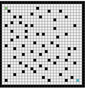
3.2.4 Random Dots, Size 30x30 . . . 46
3.2.5 Four Walls with a Wiggled Lane, Size 20x20 . . . 48
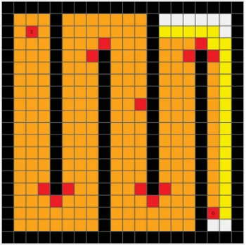
3.2.6 A Series of Walls with a Lane in the middle, Size 30x30 . . . 50
3.2.7 Maze, Size 30x30 . . . 52
3.2.8 Potential Well, Size 30x30 . . . 54
3.3 Analysis . . . 56
3.4 Conclusion . . . 57
4 APF-Optimal Search 59 4.1 Overview . . . 59
4.2 Potential Field with Optimal Search . . . 59
4.2.1 Safety Factor . . . 60
4.2.2 The Basic Artificial Potential Field Generator . . . 62
4.2.3 Linear Functions . . . 64
4.2.4 Hyperbola function . . . 67
4.2.5 Sigmoid Function . . . 67
4.2.6 Double Thresholds . . . 69
4.2.7 Comparison with Related Study . . . 70
4.3 Alternative Heuristics . . . 72
4.3.1 Sharp Bend Problem . . . 72
4.3.2 Dynamic Attractive Point of the Artificial Potential Field . . . . 73
4.3.3 The Angular Factor in Optimal Search . . . 74
4.3.4 Involving the Angular Factor in the Search Algorithm . . . 75
4.3.5 The Second Key Value . . . 75
4.3.6 Unified Key with Separate Coefficients . . . 75
4.3.7 Alternative Heuristic Function . . . 76
4.4 Line-of-sight . . . 78
4.4.1 Simple Line-of-Sight Checking for Vertex-based Search . . . 79
4.4.2 Modified Bresenham’s Algorithm for Line-of-Sight Detection . . 80
4.4.3 Obstacle as Polygon . . . 83
4.4.4 Modified Cohen-Sutherland Algorithm . . . 85
5 Building Robot Behaviours 89 5.1 Generic Strategies . . . 89
5.1.1 Target Pursuing . . . 89
5.1.2 Obstacle Avoidance . . . 90
5.2 Attacker Strategies . . . 92
5.2.1 Dynamic Attacking Position . . . 92
5.2.2 Finite State Machine for Attacker Intelligence . . . 93
5.3 Goal Keeper Strategies . . . 94
5.3.1 Defensive Blocking Position . . . 94
CONTENTS V
5.3.3 Finite State Machine for Keeper Intelligence . . . 95
6 Simulation Platform 97 6.1 Implementing System Dynamics . . . 97
6.1.1 Collision Detection . . . 99
6.1.2 The Force and the Impulse Direction . . . 102
6.1.3 Applying the Artificial Potential Field . . . 104
6.2 Implementation Details . . . 105
6.2.1 Grid mapping and Dynamic Cell Size . . . 105
6.2.2 Use of the Artificial Potential Field . . . 106
6.2.3 Multi-Linked List . . . 106
6.3 Architecture Design . . . 106
6.3.1 Main-loop and FPS Limits . . . 107
6.3.2 Structure of the Rigid Body Management . . . 108
6.3.3 Messages and Event Handling . . . 111
7 Experiments 113 7.1 Experiment Introduction . . . 113
7.1.1 Platform of the Search Algorithm Experiment . . . 113
7.1.2 Definitions and the Statistics . . . 113
7.1.3 Safety Factor of the Potential Field . . . 114
7.2 APF-Optimal Search . . . 114
7.2.1 Comparison Between the APF-A* and the Original A* . . . 115
7.2.2 One Big Obstacle in the Centre, Size 20x20 . . . 117
7.2.3 Four Medium Obstacles, Size 20x20 . . . 119
7.2.4 Five Small Obstacles, Size 20x20 . . . 121
7.2.5 Random Dots, Size 30x30 . . . 123
7.2.6 Four Walls with a Wiggled Lane, Size 20x20 . . . 125
7.2.7 A Series of Walls with a Lane in the Middle, Size 30x30 . . . 127
7.2.8 Maze, Size 30x30 . . . 129
7.2.9 Potential Well, Size 30x30 . . . 131
7.2.10 Trap, Size 30x30 . . . 133
7.2.11 GNRON Case . . . 135
7.2.12 Summary . . . 137
7.3 APF Generator . . . 137
7.3.1 The Distribution of the Magnitude Using Different Generators . 138 7.4 Comparison with Other Studies . . . 142
7.4.1 Experiments . . . 142
7.5 Robot Behaviours . . . 146
7.5.1 Platform Introduction . . . 146
7.5.2 Experiments of the Performance . . . 147
7.5.4 Summary . . . 159
7.6 Analysis and Discussion . . . 160
7.6.1 The Performance of the APF-Optimal Search Algorithms . . . . 160
7.6.2 The Performance of the Artificial Potential Field Generator . . . 160
7.6.3 The Performance of the Line-of-sight Algorithms . . . 161
7.6.4 The Effects of Using the Safety Factor on Performance . . . 161
8 Conclusion 165 8.1 Future Works . . . 167
8.1.1 Alternate Optimal Search Algorithms . . . 167
8.1.2 Decision Making . . . 167
8.1.3 Use of Fuzzy System with Artificial Potential Field . . . 168
8.1.4 A* Search in Vector Space . . . 168
List of Figures
2.1 A directed map for dijkstra algorithm . . . 8
2.2 Step 1 - Insert node A into S as initial . . . 10
2.3 Step 2 - Pop A and insert B, C into S . . . 10
2.4 Step 3 - Pop C which cost is 2, insert D, E . . . 11
2.5 Step 4 - Pop E, insert F, but not end . . . 11
2.6 Step 5 - Pop B, D is inS but no update . . . 12
2.7 Step 6 - Pop D, F is inS which has new lower cost . . . 12
2.8 The initial status of A* Search . . . 15
2.9 Two successors of S . . . 16
2.10 Only one new node, the other are blocked . . . 17
2.11 Further step . . . 17
2.12 A 2D-Plain with obstacle . . . 18
2.13 The cell partly or totally covered by the obstacle are marked . . . 19
2.14 The marked cells are blocked after removing the obstacle . . . 19
2.15 The original field that has not been divided by the grid . . . 20
2.16 Search based on the vertices . . . 21
2.17 Search based on the cells . . . 21
2.18 A path between A4 and D1 is valid . . . 22
2.20 The same path of the figure 2.19 could be smoothed . . . 22
2.19 The path found by A* is wiggled . . . 23
2.21 A possible path found by Theta* Search . . . 24
2.22 Examine the vertex D2 . . . 25
2.23 Visit the successor of D2: C2 and D3 . . . 25
2.24 Examining the line-of-sight from E1 to the successors . . . 26
2.25 Remove D2 on the path since there is a line-of-sight . . . 26
2.26 Search has be advanced to D4 . . . 27
2.27 Checking the line-of-sight for the successors of D4 . . . 27
2.28 The line-of-sight examining for the successors of C5 is from D4 but not E1 28 2.29 Magnitude of the APF . . . 31
2.30 Target is not reachable due to the obstacles around . . . 32
2.31 Size of the field . . . 35
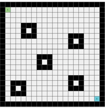
3.1 Black cells are blocked, light green is the start cell and cyan is the goal
cell . . . 39
3.2 A sample path found by a search algorithm . . . 39
3.3 Test map of a big obstacle in the centre . . . 41
3.4 The path found by A* Search . . . 41
3.5 The path found by Theta* Search . . . 41
3.6 The map of 4 medium obstacles . . . 43
3.7 The path found by A* Search . . . 43
3.8 The path found by Theta* Search . . . 43
3.9 The map of 5 small obstacles . . . 45
3.10 The path found by A* Search . . . 45
3.11 The path found by Theta* Search . . . 45
3.12 The ma of a set of dots . . . 47
3.13 The path found by A* Search . . . 47
3.14 The path found by Theta* Search . . . 47
3.15 The map of 4 walls with a wiggled lane . . . 49
3.16 The path found by A* Search . . . 49
3.17 The path found by Theta* Search . . . 49
3.18 The map of multiple walls with a lane in the middle . . . 51
3.19 The path found by A* Search . . . 51
3.20 The path found by Theta* Search . . . 51
3.21 The map of maze . . . 53
3.22 The path found by A* Search . . . 53
3.23 The path found by Theta* Search . . . 53
3.24 The map have a potential well . . . 55
3.25 The path found by A* Search . . . 55
3.26 The path found by Theta* Search . . . 55
4.1 The shortest path vs. The safest path . . . 61
4.2 The distance from s to the obstacles . . . 63
4.3 The diagram of the margin function . . . 64
4.4 Search with Margin function . . . 64
4.5 The drawback of margin function . . . 64
4.6 The gray scale illustrates the magnitude of the artificial potential field . 65 4.7 The diagram of the linear function . . . 65
4.8 Manhattan Distance . . . 66
4.9 Manhattan Distance plus artificial potential field magnitude . . . 66
4.10 The diagram of the hyperbola function . . . 67
4.11 The diagram of the sigmoid function . . . 68
4.12 The gap where the robot cannot pass . . . 69
LIST OF FIGURES IX
4.14 According to the study in [51], the position relationship between the
robot, goal and obstacle in 1-D scenario. . . 70
4.15 According to the study in [51], the magnitude distribution of the APF in 1-D scenario. . . 71
4.16 The magnitude distribution by linear function . . . 71
4.17 The magnitude distribution by hyperbola function . . . 72
4.18 The magnitude distribution by Sigmoid function . . . 72
4.19 The sharp bend in the path . . . 73
4.20 Two paths have same fcost but different angular cost . . . 74
4.21 Same node may have different angular heuristic from different parent . . 76
4.22 The same path of the figure 2.19 could be smoothed . . . 79
4.23 An intermediate step when processing LOS checking . . . 79
4.24 The light gray cells are where should be examined . . . 81
4.25 The dark gray cells will not be found by the original algorithm but should be examined . . . 83
4.26 The intersection between a segment and a polygon . . . 84
4.27 The flags of the Cohen-Sutherland Algorithm . . . 85
5.1 The flow chat of path planning and re-planning . . . 90
5.2 A possible path found by the A* Search . . . 91
5.3 The distribution of the artificial potential field around the obstacle 2 . . 91
5.4 The expected actual trail of the agent . . . 92
5.5 The attacking position . . . 93
5.6 The states and transition conditions of the attacker . . . 93
5.7 Moving to the blocking position E for coming attacking . . . 95
5.8 The states and transition conditions of the keeper . . . 96
6.1 Use 5 parameters to describe a rectangle . . . 98
6.2 Two rectangles are overlapped . . . 99
6.3 The distance between a circle and a rectangle . . . 100
6.4 Determine which quadrant the circle belongs to . . . 101
6.5 The left object hits the right one . . . 103
6.6 To determine if need to compute virtual force . . . 105
6.7 The main-loop of the simulation . . . 107
6.8 The class diagram of rigid body management . . . 108
6.9 The procedure of poll event . . . 112
7.1 The original A* Search . . . 115
7.2 The APF-A* Search . . . 115
7.3 The original A* Search with one dot in the middle . . . 116
7.4 The APF-A* Search with one dot in the middle . . . 116
7.6 A big obstacle in the centre of the field . . . 117
7.7 Path found by APF-A* Search without SF . . . 117
7.8 Path found by APF-A* Search with SF . . . 117
7.9 Path found by APF-Theta* Search without SF . . . 117
7.10 Path found by APF-Theta* Search with SF . . . 117
7.11 Four medium obstaces . . . 119
7.12 Path found by APF-A* Search without SF . . . 119
7.13 Path found by APF-A* Search with SF . . . 119
7.14 Path found by APF-Theta* Search without SF . . . 119
7.15 Path found by APF-Theta* Search with SF . . . 119
7.16 Five small obstacles . . . 121
7.17 Path found by APF-A* Search without operator factor . . . 121
7.18 Path found by APF-A* Search with operator factor . . . 121
7.19 Path found by APF-Theta* Search without operator factor . . . 121
7.20 Path found by APF-Theta* Search with operator factor . . . 121
7.21 A set of dots placed randomly . . . 123
7.22 Path found by APF-A* Search without SF . . . 123
7.23 Path found by APF-A* Search with SF . . . 123
7.24 Path found by APF-Theta* Search without SF . . . 123
7.25 Path found by APF-Theta* Search with SF . . . 123
7.26 Four walls and a wiggled path . . . 125
7.27 Path found by APF-A* Search without SF . . . 125
7.28 Path found by APF-A* Search with SF . . . 125
7.29 Path found by APF-Theta* Search without SF . . . 125
7.30 Path found by APF-Theta* Search with SF . . . 125
7.31 A series of walls with a lane in the middle . . . 127
7.32 Path found by APF-A* Search without SF . . . 127
7.33 Path found by APF-A* Search with SF . . . 127
7.34 Path found by APF-Theta* Search without SF . . . 127
7.35 Path found by APF-Theta* Search with SF . . . 127
7.36 The maze which is the most complex terrian . . . 129
7.37 Path found by APF-A* Search without SF . . . 129
7.38 Path found by APF-A* Search with SF . . . 129
7.39 Path found by APF-Theta* Search without SF . . . 129
7.40 Path found by APF-Theta* Search with SF . . . 129
7.41 The potential well that the agent will be trapped in the middle . . . 131
7.42 Path found by APF-A* Search without SF . . . 131
7.43 Path found by APF-A* Search with SF . . . 131
7.44 Path found by APF-Theta* Search without SF . . . 131
7.45 Path found by APF-Theta* Search with SF . . . 131
LIST OF FIGURES XI
7.47 Path found by APF-A* Search without SF . . . 133
7.48 Path found by APF-A* Search with SF . . . 133
7.49 Path found by APF-Theta* Search without SF . . . 133
7.50 Path found by APF-Theta* Search with SF . . . 133
7.51 Path found by APF-A* Search with SF . . . 135
7.52 Path found by Original A* Search . . . 135
7.53 Magnitude distribution . . . 136
7.54 Distribution of the linear function . . . 138
7.55 Distribution of the hyperbola function to the power of -2 . . . 139
7.56 Distribution of the hyperbola function to the power of -1 . . . 139
7.57 Distribution of the sigmoid function . . . 140
7.58 Comparison between the functions . . . 141
7.59 The scenario of GNRON problem from the study in [51] . . . 142
7.60 The performance of the APF-A* Search without SF . . . 143
7.61 The performance of the APF-A* Search with SF . . . 143
7.62 The performance of the Theta* Search without SF . . . 143
7.63 The performance of the APF-Theta* Search with SF . . . 143
7.64 The path planning demonstration from the study in [5] . . . 144
7.65 The performance of the APF-A* Search without SF . . . 144
7.66 The performance of the APF-A* Search with SF . . . 144
7.67 The performance of the APF-Theta* Search without SF . . . 145
7.68 The performance of the APF-Theta* Search with SF . . . 145
7.69 Sample performance of the Robots . . . 147
7.70 The path found by the APF-A* Search with SF . . . 149
7.71 The path found by the APF-Theta* Search with SF . . . 150
7.72 The attacking and the defense . . . 151
7.73 The path found by the APF-A* Search with SF . . . 152
7.74 The path found by the APF-Theta* Search with SF . . . 152
7.75 The path found by the APF-A* Search with SF . . . 154
7.76 The path found by the APF-Theta* Search with SF . . . 154
7.77 The defense of the keeper . . . 155
7.78 The path found by the APF-A* Search with SF . . . 156
7.79 The path found by the APF-Theta* Search with SF . . . 156
7.80 The re-planning of the attacker after the keeper push the ball away . . . 157
List of Tables
2.1 gcost and heuristic of new search nodes . . . 27
3.1 Statistics in the case of Big Obstacles . . . 40
3.2 Statistics in the case of Four Medium Obstacles . . . 42
3.3 Statistics in the case of Five Small Obstalces . . . 44
3.4 Statistics in the case of Random Dots . . . 46
3.5 Statistics in the case of Four Walls with a Wiggled Lane . . . 48
3.6 Statistics in the case of Walls with a Lane in the Middle . . . 50
3.7 Statistics in the case of Maze . . . 52
3.8 Statistics in the case of Potential Well . . . 54
3.9 Statistics of the Performance Ratios between the Optimal Searches . . . 56
4.1 Search nodes at first step . . . 77
4.2 Angular Factors . . . 77
4.3 gcost and heuristic of all the nodes . . . 77
7.1 Statistics of the Performances of APF-Optimal Searches with or without SF, in the case of Big Obstacle . . . 118
7.2 Statistics of the Performances of APF-Optimal Searches with and with-out SF, in the case of Four Medium Obstalces . . . 120
7.3 Statistics of the Performances of APF-Optimal Searches with and with-out SF, in the case of Five Small Obstalces . . . 122
7.4 Statistics of the Performances of APF-Optimal Searches with and with-out SF, in the case of Random Dots . . . 124
7.5 Statistics of the Performances of APF-Optimal Searches with and with-out SF, in the case of Four Walls with a Wiggled Lane . . . 126
7.6 Statistics of the Performances of APF-Optimal Searches with and with-out SF, in the case of Walls with a Lane in the Middle . . . 128
7.7 Statistics of the Performances of APF-Optimal Searches with and with-out SF, in the case of Maze . . . 130
7.8 Statistics of the Performances of APF-Optimal Searches with and with-out SF, in the case of Potential Field . . . 132
7.9 Statistics of the Performances of APF-Optimal Searches with and with-out SF, in the case of Trap . . . 134
7.10 Statistics of the Performances of APF-Optimal Searches with and with-out SF, in the case of Replicated Environment from the Study by Ge & Cui in 2000 . . . 143 7.11 Statistics of the Performances of APF-Optimal Searches with and
with-out SF, in the case of the Replicated Environment from the Study by
Li, Yamashita, Asama & Tamura in 2012 . . . 145 7.12 Statistics of the Performances of APF-Optimal Searches with SF, in the
case of the Potential Well running on the Simulator . . . 150 7.13 Statistics of the Performances of APF-Optimal Searches with SF, in the
case of the Multiple Walls with a Lane inthe Middle running on the Simulator . . . 153
7.14 Statistics of the Performances of APF-Optimal Searches with SF, in the case of the GNRON problem running on the Simulator . . . 155 7.15 Statistics of the Performances of APF-Optimal Searches with SF, in the
case of the Cross Blocks running on the Simulator . . . 157 7.16 Statistics of the Performances of APF-Optimal Searches with SF, in the
case of the Random Obstacles running on the Simulator . . . 158 7.17 Comparison Between Original A* and APF-A* SF, in the case of One
Big Obstacle, according to the figures 3.4 and 7.8 . . . 161 7.18 Comparison Between Original A* and APF-A* SF, in the case of Four
Medium Obstacles, according to the figures 3.7 and 7.13 . . . 162
7.19 Comparison Between Original A* and APF-A* SF, in the case of Five Small Obstacle, according to the figures 3.10 and 7.18 . . . 162 7.20 Comparison Between Original A* and APF-A* SF, in the case of
Ran-dom Dots, according to the figures 3.13 and 7.23 . . . 162 7.21 Comparison Between Original A* and APF-A* SF, in the case of Four
Walls with a Wiggle Lane, according to the figures 3.16 and 7.28 . . . . 163 7.22 Comparison Between Original A* and APF-A* SF, in the case of Walls
with a Lane in the Middle, according to the figures 3.19 and 7.33 . . . . 163 7.23 Comparison Between Original A* and APF-A* SF, in the case of Maze,
according to the figures 3.22 and 7.38 . . . 163
7.24 Comparison Between Original A* and APF-A* SF, in the case of Poten-tial Well, according to the figures 3.25 and 7.43 . . . 164
Abstract
The artificial potential field (APF) is a popular method of choice for robot navigation, as it offers an intuitive model clearly defining all attractive and repulsive forces acting on the robot [3] [25] [29] [43] [50]. However, there are drawbacks that limit the usage
of this method. For instance, the local minima problem that gets a robot trapped, and the Goal-Non-Reachable-with-Obstacle-Nearby (GNRON) problem, as reported in [51] [5] [23] [2] and [3]. In order to avoid these limitations, this research focuses on devising a methodology of combining the artificial potential field with a selection of optimal search algorithms. This work investigates the performance of the method when using
different optimal search algorithms such as the A* algorithm and the any-angle path-planning Theta* Search, in combination with different types of artificial potential field generators. We also present a novel integration technique, whereby the Potential Field approach is utilized as an internal component of an optimal search algorithm, consid-ering the safeness of the calculated paths. Furthermore, this study also explores the
optimization of several auxiliary algorithms used in conjunction with the APF-Optimal search integration: There are three different methods proposed for implementing the line-of-sight (LOS) component of the Theta* search, namely the simple line-of-sight checking algorithm, the modified Bresenham’s line algorithm and the modified Cohen-Sutherland algorithm. Contrary to the studies presented in [5], [42], [48] and [40] where the APF and the optimal search algorithms were used separately, in this research, an
integrative methodology involving the APF inside the optimal search with a newly pro-posed Safety Factor (SF) is explored. Experiment results indicate that the APF-A* Search with the SF can reduce the number of state expansions and therefore also the running time up to 19.61%, while maintaining the safeness of the path, as compared to APF-A* when not using the SF. Furthermore, this research also explores how the
proposed hybrid algorithms can be used in developing multi-objective behaviours of single robot. In this regard, a robot soccer simulation platform with a physics engine is developed as well to support the exploration. Lastly, the performance of the proposed algorithms is examined under varying environment conditions. Evidences are provided showing that the method can be used in constructing the intelligence for a robot goal
keeper and a robot attacker (ball shooter). A multitude of AI robot behaviours using the proposed methods are integrated via a finite state machine including: defensive positioning/parking, ball kicking/shooting, and target pursuing behaviours.
Chapter 1
Introduction
In the robot navigation problem domain, the most fundamental research issue is how to select the appropriate motion-planning algorithm for specific working environments.
From the MIT IAP robotics course [27], various types of useful navigation algorithms can be combined together. Among these algorithms, we have the optimal search al-gorithms and the artificial potential field; they are widely used in different robotic platforms such as Unmanned Aerial Vehicle (UAV) control [3] [23], indoor robot con-trol [47] and the robot soccer game [32] [35] [36] [39] [41] [43].
There are two major components in the robot navigation problem: target pursuing and
obstacle avoidance. Target pursuing is the most fundamental one, which makes the robot move towards the target position. Then, the obstacle avoidance is involved in making the robot avoid the obstacle while pursuing the target. In order to deal with these requirements, the robot navigation problem is divided into two major aspects: path-planning and motion control. Path planning is used to find out the shortest path
from the starting position to the goal with the shortest running time that avoids all the obstacles, then the motion control is engaged to control the robot moving along the path and respond to any events happening before the robot arrives at the goal.
In this research, the methodology of using both the Artificial Potential Field (APF) and the optimal search for the robot navigation problem are investigated. Due to the limitation of using individual algorithms separately, the integration of using both the
artificial potential field and the optimal search to resolve the limitation of each other is developed and examined. To customize the results of optimal search, a concept from the artificial potential field which is called safety factor (SF) is combined into the optimal search that makes the search algorithm find out not only the shortest path but the best path which has a balance of path length and robot safety as well. Also,
alternative generator functions of the artificial potential field are studied to improve the performance of motion planning. Moreover, with the utilization of the optimal search
algorithms, the flaws of the artificial potential field are addressed.
The researches like [54] and [28] have stated that a necessary distance from the obsta-cle is essential for the path planning problem because in the real practice, the robot is not a solid point but has a volume, which means a margin to the neareast
obsta-cle is compulsory. The drawback of using constant margin will be illustrated in the section 4.2.2, and the methodology of evaluate the dynamic margin using SF will be discovered.
For the purpose of examining the efficacy of the navigation algorithms in real practice, the robot soccer game is preferred which is a suitable research platform requiring the navigation algorithms. Then, due to the complexity of the robot soccer game, multiple intelligent behaviours for the soccer players were developed and examined. Moreover,
three different line-of-sight algorithms are developed and examined, as an auxiliary component of the Theta* Search algorithm, since the literature does not provide specific details on how to actually implement it.
For better game simulation, the implementation includes physics mechanics as well as collision detection. A dynamic cell size technique for the grid-world representation is also developed, for the purpose of using optimal search in unknown terrains.
Last but not least, the performance of the navigation algorithms are compared against the experiment results from the other researches. The strengths and the limitations
of the proposed methods are also summarized, with a discussion of areas for future work.
1.1
The Problem Domain: Robot Soccer Game
The robotics soccer game is to simulate the real soccer game, which purpose is control-ling the robots to pursue and kick the ball into the gate that belongs to the opponent team, and defending the attacking from the opponent team [22]. The behaviors of the robots are controlled by the artificial intelligence automatically. The researches about the robot soccer game like [32], [36],[39] and [41] have indicated that there are
multiple abilities to play the game, such as the target pursuing, obstacle avoidance, decision making and cooperating. Moreover, each robot player requires multi-model behaviours for various tasks. For instance, the attacker should have the ability to find out a proper position to kick the ball toward the gate, which requires both the path planning [36] and the obstacle avoidance when moving to the attacking position [41].
1.2. RESEARCH OBJECTIVES 3
In the robot soccer game, one of the most important issues is the robotics navigation: first, the purpose of the path planning is to find out a proper path from the current
position of the robot to the target position which could be either the ball or the position for further attacking or defensing. Then, the algorithm of motion control should have the ability to make the robot moving along the given path and avoiding the obstacles at the same time.
There are also other problem domains of the robot soccer game like the vision
process-ing and the decision makprocess-ing [22]. These domains are combined with the navigation algorithm to manipulate the robot together. Nevertheless, this research will focus on the navigation problem only: All the other components of the robot soccer game are considered as idealized.
1.2
Research Objectives
The major purpose of this research is to investigate the efficacy of using optimal search
algorithms with the artificial potential field for the robot navigation problem. Optimal search algorithms are widely used in the area of navigation, but have drawbacks in terms of running time [8][17][42]. On the other hand, the artificial potential field is a high speed algorithm for real-time navigation but has some weaknesses.
The local minima problem is one of the the major concerns for using the artificial
potential field [5] [24]. The fundamental mechanism of the artificial potential field is to use the gradient to indicate the moving direction of the agent. However, the local minima may problem appear if there are more than one point having a zero gradient, which causes the agent has the probability of being trapped other than the goal position.
Another problem is called the Goal-Non-Reachable-with-Obstacle-Nearby ( GNRON ) problem [2]. The GNRON problem will happen if the goal position is too close to the obstacle so that the gradient at the goal position is not 0, or all the gradients of each point around the goal are all pointing away from the goal. The effect is that it prevents the agent to move towards the goal.
This research explores a proper combination of optimal search algorithms and artificial potential field to address the flaws of artificial potential field in robot navigation. Since both of the local minima and the GNRON problems could arise if there is no unique goal on the field, the optimal search algorithms are selected to indicate the only distinct goal even there are multiple or no position having zero gradient. Moreover, the methodology
and examined.
In order to implement the Theta* Search Algorithm, the study of implementing the line-of-sight component of the Theta* Search should be investigated. Due to the various types of the environment, different algorithms are developed to adapt corresponding
cases. Furthermore, the utilization and modification of existing algorithms such as the Bresenham’s Line Algorithm [12] which is used for mapping the vector graph into pixel and the Cohen-Sutherland Algorithm [14] which is to determine the necessary of rendering in the area of computer graphics will be explored to apply them for line-of-sight check.
In this research, the robot soccer game is used as platform to evaluate the performance of the study result. As it is mentioned in the section 1.1, an idealized simulation
platform of the robot socces game will be established to restrict the variation of the research. That is, the vision processing system of the robot soccer game will not be considered.
1.3
Significance of the Research
Although there have been many researches about the navigation problem in the robot soccer game, such as [32], [35] [39], [41], [43], [36], and also a lot of researches about the
navigation problem using various algorithms under different environment, for instance, the flight path planning [1], the UAV control [3], the virtual motion [45] and so on, there is few study about using the combination of multiple algorithm in the robot soccer navigation.
This research introduces a new technique of combining the A* and Theta* algorithms with the Potential Field algorithm, in order to add a safety factor to the calculated paths. The novel integration technique makes use of the Potential Field algorithm
as an internal component of the A* algorithm, whereby it is used to calculate the g-cost values, taking into account the presence of obstacles around each visited way-point.
By implementing the corresponding simulation platforms, the comparison between the performances of different algorithms are explored and exposed as well. The implemen-tation includes the mechanics engine for aspects of rigid body motion and collision detective.
In order to implement the Theta* Search, the detailed implementation of the
1.4. STRUCTURE OF THE THESIS 5
1.4
Structure of the Thesis
In the chapter 2, the theoretical framework will be introduced, plus the review of the
related literature when explaining the corresponding algorithms. The section 2.1 will introduce the A* Search Algorithm and the Theta* Search Algorithm which are based on the Dijkstra Algorithm. Then, the artificial potential field will be introduced in the section 2.2.
The chapter 3 will explore the performance of the related algorithms. The majority of the preliminary exploration is the optimal search algorithms.
In the chapter 4, the algorithm of how to combine the optimal search algorithms with the artificial potential field will be expressed and proved. The selection of the
artifi-cial potential field functions will be explored. Also, the discussion of using alternative heuristic in the optimal search are exposed as well. Furthermore, the algorithms of im-plementing the concept of line-of-sight will be introduced as well, including the modified Bresenham’s Line Algorithm and the modified Cohen-Sutherland Algorithm.
After that, the strategies of the robot soccer behaviours will be expressed in the chapter 5, including the generic strategies, the attacker strategies and the keeper strategies. The algorithms of implementing the strategies will be introduced at the same time.
In order to explore the performance of the algorithms, a platform should be constructed
as well. In the chapter 6, the implementation of experiment platform will be introduced. The section 6.1 will expose the algorithm of mechanics simulation will is focused on the collision detective and applying the motion control of the artificial potential field. Then the implementation details of the search algorithms will be discussed in the section 6.2. Then, the architecture of the platform will be exposed in the section 6.3.
The experiment result of corresponding algorithms are presented in the chapter 7. First, the performances of using different optimal algorithms with the artificial potential field
Chapter 2
Theoretical Framework and
Review of Related Literature
In general, the robot navigation problem contains two major parts: path planning and intelligent control. For path planning, the algorithms should have the ability of finding the best path from the start position two the goal. On the other hand, for the intelligent control, the algorithms should have the ability to control the motion of the robot to
move along the found path and avoid the obstacle.
These two parts are not totally individual: when a path is planned, the way-points should have a proper tolerant that allow the robot to move through, which is a partial
obstacle avoidance as well. Furthermore, the appearance of the path is generally a set of way points P ={s1, s2, ...sn}, which means the control algorithm should also plan the path between two connected way-points.
That is, the robot navigation could not be implemented by any single algorithm, but
requires a combination of multiple algorithms to cooperate.
2.1
Optimal Search Algorithms
The optimal search algorithm is a not a single algorithm, but a set of algorithms based
on the Dijkstra Algorithm [9]. The purpose of the optimal search is to find out the shortest path from the start to goal as fast as possible.
2.1.1 Dijkstra Algorithm
The Dijkstra algorithm was originally addressed and proved by Dijkstra, E. W in 1956 [6][10]. As a basis of the optimal search algorithms, this algorithm generating the search tree from a directed map. A sample directed map is shown in figure 2.1, the value of the edges is the cost of moving from one node to the connected node with given direction.
Figure 2.1: A directed map for dijkstra algorithm
In Dijkstra algorithm, the top two essential aspects are the search queue S which
is a priority queue, and the visited list V which is a set that records the node has been searched. During the search processing, the total cost from the start node to the current visited node will be used as the key value of the priority queue, and updated the smallest cost to the visited list.
The structure of a node is
1 Node :
2 Node parent := null
3 U N S I G N E D cost := + INF
2.1. OPTIMAL SEARCH ALGORITHMS 9
1 I n i t i a l i z e :
2 { S }:= null
3 { V }:= null
4 create Node n := { null ,0}
5 { S }. i n s e r t ( n )
6
7 F i n d P a t h :
8 WHILE NOT { S }. empty ()
9 u := { S }. top ()
10 { S }. pop ()
11
12 IF u is Goal THEN
13 r e t u r n u
14 ELSE
15 IF u in { V } THEN
16 N E X T L O O P
17 ENDIF
18
19 { V }. insert (u , u . cost )
20
21 F O R E A C H v as n e i g h b o u r of u
22 IF v in { S } THEN
23 IF cost (u , v ) + u . cost < v . cost THEN
24 { S }. r e m o v e ( v )
25 { S }. p a r e n t = u
26 v . cost = cost (u , v ) + u . cost
27 S . insert (v , v . cost )
28 ENDIF
29 ELSE NOT v in { V } THEN
30 v . cost = cost (u , v ) + u . cost
31 v . p a r e n t = u
32 { S }. i n s e r t ( v )
33 ENDIF
34 E N D L O O P
35 ENDIF
36 E N D L O O P
37 r e t u r n null
In the initializing phase, both the search queue and the visited list will be empty, then
smallest cost will be popped from the search list and examined. First, if the current node u is the goal node, the search will be terminated and return u as the result.
Otherwise, u will be added to the visited list, and all the neighbour nodes v will be examined.
If v has been visited, but cost of the path of moving from start through u to v is smaller than the recorded cost, then the parent of v will be replaced by u, and the cost of v will be updated as well. On the other hand, if v is a new node which has not been visited, it will be added to the search queue, and also the cost from s through u to v as the cost of v.
If any goal node has been found, by the traversal of the parent node from goal node
to start node, the shortest path will be found as well. However, if there is no result found before the search queue is empty, a result of null will be given out to indicate that there is no valid path from the start node to the goal.
In the sample of figure 2.1, assuming the requirement of the search is to find out a path from the node A and the node F. The following figures demonstrate the major steps of the search: the gray nodes are in the search list, and the cost of the nodes are listed as well.
Figure 2.2: Step 1 - Insert node A into S as initial
First, as it is shown in the figure 2.2, the node A is inserted into the search list during the initializing phase. The rest of the nodes are still in unknown status.
2.1. OPTIMAL SEARCH ALGORITHMS 11
Then the major process will start. The node which has the smallest cost will be popped and examined if it is the goal. Currently, there is only one node A in the search list,
so that A is popped and the neighbours of A, which have not been searched or visited are added to the search list, with the cost separately.
Figure 2.4: Step 3 - Pop C which cost is 2, insert D, E
Moving to the next iteration, since C has the smallest cost in the search list, it will be popped like A in previous round. The neighbours of C are inserted into the search list
as well.
Figure 2.5: Step 4 - Pop E, insert F, but not end
In the next iteration, after the node E is popped and examined, the node F which is the goal node will be added into the search list, with a cost of 11 and parent of E. However, since the goal examining will only be occurred when the node is popped from
Figure 2.6: Step 5 - Pop B, D is in S but no update
Although F has been in the search list already, there two nodes has smaller cost, and also their cost are exactly the same. Depend on the implementation of the priority queue, both of the could be popped. In this sample, B is popped first and examined, and the node D is left in the search list. Because the cost from A t D through B is 6, which is greater than the current cost of D, D will not be updated, and also no new
node will be inserted into the search list.
Figure 2.7: Step 6 - Pop D, F is inS which has new lower cost
While the node D is popped as well, as the neighbour of D, the cost of the node F will be updated since the cost through D to F is smaller than that through E to F. At the same time, the parent of F will be changed to D as well, so that the shortest path from
A to F is not A-C-E-F anymore, but A-C-D-F.
Then the final step, since there is only one node in the search list, F will be popped and returned as the final result of the entire search process.
This sample demonstrates the procedure of the Dijkstra algorithm, and also the sig-nificance of recording the cost of each node which ensuring the shortest path will be
found.
Although the Dijkstra algorithm has the ability to find out the shortest path, the
2.1. OPTIMAL SEARCH ALGORITHMS 13
O(—E— + —V—log—V—) when using fipponacci heap as the implementation of the priority queue, where V is the count of node and E is the count of edges [11].
2.1.2 A* Search Algorithm
The A* Search Algorithms is a classical search algorithm for finding out the shortest
path on a known field. It is widely used in the area of path planning for known terrain [8] [13] [16] [23].
Different from the Dijkstra algorithm, the A* Search introduced another crucial aspect: heuristic. In the A* Search, an evaluated cost from a node n to the possible target node t is established by the heuristic function ˆh(n)≤h(n, t), which had been proved by Hart, Nilsson and Raphael in 1968 [9], where h(n, t) is the actual shortest cost from n to t.
This condition is also known as the consistency of the heuristic [9]. In the original algorithm, the heuristic is evaluated by the euclidean distance d(x,y) from the current node to the target node t.
Another aspect used in the A* algorithm is the expanded list{E}, which is also known as close set. Different from the visited list in the Dijkstra algorithm, a node will be
expanded if and only if the shortest path from the start node to this node has been found. The condition of using expand list is the consistency heuristic, which had been proved by Hart, Nilsson and Raphael as well [9].
In order to simplify the computation work in practice, the search node is introduced. The search node is defined as a series of connected nodes which present that path from the back one to the front one. For example in the figure 2.1 on page 8, a search node
s={DCA}indicates that there is a path from the node A through C to the node D. Furthermore, the evaluated cost of this search node ˆf(s) =g(s) + ˆh(s) is also used as the key value in the search list, as result, a complete search node will be marked like
s={8DCA}, where theg(D) = 5 and ˆh(D) = 3.
The search list {S}of the A* algorithm is the same as that in the Dijkstra algorithm, which is a priority queue as well. Furthermore, the expanded list in the A* algorithm
is a set which ensures no duplicate expand may happen.
1 S e a r c h N o d e {
2 U N S I G N E D g co st := + INF
3 U N S I G N E D h co st := + INF
4 { N } as Node := null
5 }
6 G e t K e y S e a r c h N o d e N :
7 r e t u r n N . gcost + N . hcost
8
9 I n i t i a l i z e :
10 { S } := null
11 { E } := null
12 Create Search Node N
13 N . gcost = 0
14 N . Add ( start )
15 N . hcost = d i s t a n c e ( start , goal )
16 S . i n s e r t ( G e t K e y ( N ) , N )
1 F i n d P a t h :
2 WHILE NOT { S }. empty ()
3 M = { S }. front ()
4 { S }. pop ()
5 Node u = M . last ()
6 IF u is goal THEN
7 r e t u r n M
8 ENDIF
9
10 { E }. i n s e r t ( u )
11 F O R E A C H v is s u c c e s s o r of u
12 IF v in { E } THEN
13 N E X T L O O P
14 ENDIF
15
16 Crate Search Node N := M
17 N . Add ( v )
18 N . g co st += d i s t a n c e ( u , v )
19 N . hcost := d i s t a n c e (v , goal )
20 { S }. i n s e r t ( G e t K e y ( N ) , N ) 21 E N D L O O P
22 E N D L O O P
2.1. OPTIMAL SEARCH ALGORITHMS 15
During the initialization phase of the A* algorithm, both the search list {S}and the expand list {E} are cleared, and then the first search node N is created. The start node will be added to the search node, and the gcost of N is set to 0 since there is no actual cost. After that, the heuristic function is applied, which is the distance between the start node and the goal node. At last, the initial search node N will be inserted into {S}, with its fcost as the key value.
When processing the search, at each iteration, the search node M with a key value is the smallest in the search list will be popped and examined. The last added node in
M, u, will be compared with the goal node to determine if M is the shortest path found or not. If the node u is not the goal node, it will be expanded immediately, and then all the successors of u will be examined.
The existence in the expanded list of each successor will be checked at this step, and new a search node N is created only for the successor that has not been expanded. The initial value of N is a copy of the search node M, then the successor v will be added to
the end of N, and the actual cost from node u to v will be added the gcost of N. The heuristic of N is also need to be replaced by the hcost of the node v but not u anymore. Then the final step is to add the new search node N back to the search list {S}, and moving to the next iteration.
Figure 2.8: The initial status of A* Search
Figure 2.8 demonstrates an initial state of the A* search, where A1 ( marked as S ) is the start node and D3 ( marked as G ) is the goal node. The search is restricted to 4-connected, that is only the nodes have shared edge are connected together. The distance between connected nodes is set as 1 as well. In order to simplify the computation, the manhattan distance is also used to replace the euclidean distance, which is defined as
the equation 2.1
Figure 2.9: Two successors of S
In the main procedure of the search, the search node with the lowest cost will be popped from the list. As it is shown in the figure 2.9, the search node M = 2S is popped, then
the last element in the this search node u = S is examined that if it is the goal node or not. Since the goal node is D3 but not S, S is inserted into the expand list, and then the successors of S, B1 and A2, will be selected and checked as well.
Because both B1 and A2 have not been expanded yet, which means the shortest path from S to these two nodes are not found, two new search nodes are generated by extending the path to them separately. For the first new search node S-B1, the gcost is 0+1, where 0 is the gcost of the previous search node S, and 1 is the cost from S to B1. Then the hcost is the manhattan distance from the node B1 to G which is 2, as a
result, the fcost of S-B1 is 3.
The same processing is also applied to the other new search node S-A2 which fcost is 4 = 1+3. After the successor is processed, the new search node is inserted back to the search list.
After all the successors have been processed, the procedure is moved to the next itera-tion and the first step is repeated. Since the original search node 3S has been removed already, currently, the search node with the lowest cost is 3S-B1. As a result, this search
2.1. OPTIMAL SEARCH ALGORITHMS 17
Figure 2.10: Only one new node, the other are blocked
Figure 2.11: Further step
The following processing are illustrated in the figure 2.10 and the figure 2.11. For the search node 3S-B1, since only one successor is accessible, the new search node is
generated as 3S-B1-C1, with a cost is still smaller than 4S-A2 generated in the previous iteration. As a result, 3S-B1-C1 will be popped before 4S-A2, and the further process is based on the node C1 but not A2.
2.1.3 Object Representation in the 2D Gridworld
In general, the A* search is mainly focussed on the path finding in euclidean space,
that v=r θ
The 2D search field is defined as a 2D-plane, which divided by numbers of lines along x and y axis. The neighbour grids are connected. The cell is defined as the smallest
rectangles on the field crossing by the lines, and the vertex, or the grid is the intersection point of the lines.
There will also be obstacles on the search field. In order to simplify the computation,
The following figures 2.12, 2.13 and 2.14 illustrate a 2D search field that which has been divided by the lines with an obstacle on it.
Figure 2.12: A 2D-Plain with obstacle
The cells which are partly or totally covered by the obstacle are marked as gray, which
2.1. OPTIMAL SEARCH ALGORITHMS 19
Figure 2.13: The cell partly or totally covered by the obstacle are marked
After removing the obstacle, the blocked cells have replaced, where any path that may go through them are not allowed.
2.1.4 Search in Vertex-Based and Cell-Based Worlds
When searching path on the search field, in general, there are two methods to mark the node. Considering the sample illustrated in the figure 2.15, assuming the requirement of
the search algorithm is to find out the path from the top-left corner to the bottom-right corner.
Figure 2.15: The original field that has not been divided by the grid
After dividing the search field, the next option is to decide whether the search is based on the cells or based on the vertices. For instance, in the figure 2.16, the coordinate C-3 represents a vertex, but in the figure 2.17, the coordinate C-3 represents a cell.
The cell of the search field is defined as the minimum rectangle area, which is crossed by four edges. The cell based search will find out a path which is a series of connected
cell. The vertex of the search field is defined as a intersection point of the search field. The vertex based search will find out a series of connected vertices as the path.
The major difference between them is the cell represents an area, that there may be some information missed or ignored during the search. For instance, consider the cell B2 in the figure 2.17, since it is blocked due to the obstacle, it will not belong to any of the path. However, the vertices and edges of this blocked cell are still accessible if
2.1. OPTIMAL SEARCH ALGORITHMS 21
Figure 2.16: Search based on the vertices
Figure 2.17: Search based on the cells
and B2 are two vertices that belong to the blocked cell.
Since most of the searches on the 2D-field are to find out the shortest path between two point, the vertex based search is more suitable because all the search nodes are
considered as a point but not a rectangle area. In the following chapters, all the search will be based on the vertex if there is no specification.
2.1.5 Any-Angle Search and the Line-of-sight
In the A* search, the angle relationships between neighbour nodes on the path are
concentrated on vertical, horizontal or diagonal, because the successors are physically connect to the source node. Consider the sample illustrated in the figure 2.19, the shortest path found by A* from A1 to H5 is A1-B2-C2-D3-E3-F4-G4-H5.
Figure 2.18: A path between A4 and D1 is valid
Figure 2.20: The same path of the figure 2.19 could be smoothed
The concept of line-of-sight is introduced by Yap, 2002 [17], with the purpose of re-moving the unnecessary intermediate node on the path. The algorithm of examining line-of-sight depends on how the search field is divided, or how the obstacle is de-fined.
2.1. OPTIMAL SEARCH ALGORITHMS 23
Figure 2.19: The path found by A* is wiggled
2.1.6 Post-smoothing of the A* Search Algorithm
The purpose of Post-smoothing is to remove the unnecessary way point on the path found by the A* search [20]. As soon as a valid path has been found by the A* search, the Post-smoothing is executed. Assuming the way points of the path is connected as a linked-list, the post-smoothing is to remove some of the way points:
ExistP ath:={S0, S1, ...Sn} FOREACH s∈(P ath\ {S0, Sn})
sp:=s.P rev
sn:=s.N ext
IFLineOf Sight(sp, sn) THEN
RemoveF romP ath(s) End IF
ENDLOOP
The Post-smoothing reduces the count of the way points on the path. However, it also increases the workload of the search since the line of sight checking is only applied after
the path is found.
2.1.7 Theta* Search Algorithm
Theta* search is an alternative version of A* search, which was introduced by Daniel, K, Nash, A, Koenig, S and Felner, A in 2010. The basic idea of Theta* search is to remove a constraint of 8-edges A* search that all the path nodes must be the neighbour
of their parent nodes and their child nodes.
s from the search node S will be examined, then the successors which has not been expanded will be joined into the search node S to generate new search nodes S’, and
then S’ will be added into the self-sorted search list. In this procedure, when a new search nodes is generated, the latest path node will always be the neighbour of previous path node, that is, the direction between two connected node will be concentrated to vertical, horizontal or 45-degrees.
Figure 2.21: A possible path found by Theta* Search
Different from the A* algorithm, Theta* algorithm involves an extra examining during this procedure: the line-of-sight checking[15] between the parent node of current, and
the successor.
The figure 2.21 illustrates a possible result path found by the Theta* Search Algorithm
from E1 to A5. By applying the feature of line-of-sight checking, the path is not concentrated to certain angles anymore.
Considering the case shown in the figure 2.22: find out the path from E1 to A5. In A* Search with 8-connected node, an possible result path would be E1-D2-D3-D4-C4-B4-A5. Same as the A* Search, the Theta* search will begin from checking the successors of the start node E1. Assuming the euclidean distance (d(s, s) =
2.1. OPTIMAL SEARCH ALGORITHMS 25
Figure 2.22: Examine the vertex D2
Figure 2.23: Visit the successor of D2: C2 and D3
Then the successors of D2: both C2 and D3 have the smallest heuristic value, so that new search nodes C2-D2-E1 and D3-D2-E1 might be added to the search list with the same fcost.
Before adding the new nodes to the search list, the Theta* search will process the line-of-sight checking from the parent of current node D2 to the successors C2 and D3. As it is shown in the figure 2.23, the line-of-sight checking is applied between (E1, C2) and (E1, D3).
Since both of the results of line-of-sight checking are true, the current node D2 will be removed from the search nodes, and the new search nodes will be update to E1-C2 and
Figure 2.24: Examining the line-of-sight from E1 to the successors
Figure 2.25: Remove D2 on the path since there is a line-of-sight
The next iteration will repeat the same procedure. Since the search node E1-C2 and E1-D3 have the same fcost, one of the will be popped from the search list depend on the implementation. Assuming E1-D3 will be popped first, then the successor of D3 will be checked and the search will advance.
Figure 2.26 illustrates that the search has advanced to where D4 has been expanded,
and successors of D4 are going to have the line-of-sight checking. Although there is only one successor C3 is blocked, to simplify the demonstration, only C4, C5 and D5 are considered due to the low heuristics of them.
Checking the successors C4, C5 and D5, as it is illustrated in the figure 2.27: the line-of-sight checking from E1 to them are not all success. There are not sights from E1 to
2.1. OPTIMAL SEARCH ALGORITHMS 27
Figure 2.26: Search has be advanced to D4
Figure 2.27: Checking the line-of-sight for the successors of D4
of these search nodes.
Table 2.1: gcost and heuristic of new search nodes
heuristic gcost E1-D4-C4 √5 √10 + 1 E1-D4-C5 2 √10 +√2
E1-D5 3 √17
When C4 or C5 is expanded, like the sample in the figure 2.28, the line-of-sight checking will be from the parent of C4 or C5, which is D4 but not E1, to the successors.
Comparing with original A* search, Theta* search results a much smoother path, how-ever, due to the extra examining procedure during the search, the run time is not
Figure 2.28: The line-of-sight examining for the successors of C5 is from D4 but not E1
2.1.8 Limitations of the Optimal Search Algorithms
The search algorithms have a limitation of cannot cope with dynamic environment. While the agent is moving along the path found by the search algorithm before starting, the environment may not be changed, otherwise the previous path could be overlapped
by the obstacle. Van Toll & Geraerts exposed an improvement of the search algorithm for dynamic environment in 2015[4], which is to detect the change of the environment at each iteration and do re-planning by reusing part of the previous path. However, there is no guarantee of the performance if there are multiple changes happening in same iteration.
There is another research by Wang, Zhou, Zheng & Liang in 2014 use Hierarchical A* Search for navigation for complex environment [8], and also a similar research by Yap,
Burch, Holte, Schaeffer in 2011 called Block A* Search [17]. Both of them divided the search field in several blocks to reduced the complexity of planning and re-planning by reusing the known information of the field. However, if most of the obstacles are moving, or most of the blocks are changed frequently, re-initializing is neccesary, without any guarantee about the speed as well.
The research by Pochmara, Grygiel, Koppa & Kaminski in 2013 expressed the perfor-mance of the A* Search in real-time navigation. With different distance functions, the
2.2. THE ARTIFICIAL POTENTIAL FIELD ALGORITHM 29
2.2
The Artificial Potential Field Algorithm
The artificial potential field was introduced by Oussama Khatib, 1985. The original idea of artificial potential field is to generate a virtual field in the space, all the target objects which need to be manipulated will be affected by this virtual field. The artificial potential field is a simulating of the natural potential fields like gravity field, which apply a virtual force to the target objects, so that the motion of objects will be affected by the virtual force.
The types of artificial potential field could vary. The most fundamental type is a point that generates a scalar field where the magnitude is inversely proportional to
the square distance. Also, the magnitude is not constrained to that, but could be self-defined depend on the circumstances. The other types could be considered as the combination of multiple fundamental potential fields. The magnitude of an artificial potential field at point k could be presented as the equation 2.2:
N(k) =
P(x, y)dxdy. (2.2)
In equation 2.2, P(x,y) is the magnitude which is generated by the point (x,y) to target point k, and P is the pre-defined generator function. Furthermore, for discretization, the artificial potential field could be considered as a sum magnitude of multiple objects that generate separate artificial potential field affecting the point k at same time, so
that the magnitude at point s is:
m(s) = n
i=1
Pi(s). (2.3)
2.2.1 Artificial Potential Field for Navigation
Considering the equation 2.3: the scalar field also generate the vector field of the gradient, which is how the artificial potential field affects the moving objects. For each
point s on the artificial potential field, the gradient at s determines the force affected on the agent x placed at s, both the direction and the magnitude:
−−→
a(x) =
−−−→
F(x)
mx
= P(ks
mx
. (2.4)
the newtons law of motion, there will be :
vx(t) =
t1
t0
a(x)dt+vx(0),
Sx(t) =
t1
t0
v(x)dt+Sx(0).
(2.5)
According to the equation 2.5, for the case of static field where the obstacle are not movable, the path S could be determined as soon as the start and the goal position are set. That is, the artificial potential field have the ability of path-planning for static
field.
However, if the field is dynamic and the motion status of the obstacles are unknown, the path-planning of the artificial potential field does not work. That is, there is an assuming of the artificial potential field that during t0 → t1, the field should be static.
2.2.2 Simplification of the Artificial Potential Field
In most of the cases, the obstacles are not points but have a shape. A set of the points where the distance from the point to the obstacle are the same are supposed to have the same magnitude on the potential field. If the magnitude is proportional to the
distance, then the gradient of the potential field generated by this obstacle will have an attractive force [19]. Oppositely, as the magnitude is inversely proportional to the distance, the obstacle will have repulsive force [19].
This simplification is because the major purpose of the potential field is to add an extra virtual force that makes the object to have a tendency to move towards or away from the obstacle. Since for any curve the distance from a point outside to the curve is the
straight line orthogonal to the curve passing through the point, the computation of the magnitude of the potential field could be reduced to only two parts: the distance from the target agent to the obstacles, and the direction from the edge of the obstacles to the agent.
In the case of multiple obstacles, this simplification also have the effect that, the mag-nitude at point k is proportional or inversely proportional to the minimum distance
2.2. THE ARTIFICIAL POTENTIAL FIELD ALGORITHM 31
2.2.3 Limitations of the Artificial Potential Field
Although the artificial potential field could be used for navigation, it has some limita-tions that cannot deal with the navigation problem in complex environment.
Potential Well
The concept of potential well is the main reason of this limitation: since the motion of agent on potential field is based on the gradient, and gradient of the artificial potential
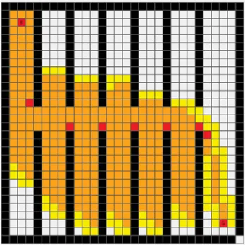
field is a vector field, there could be 0, 1 or multiple points on the artificial potential field where the magnitude is 0.
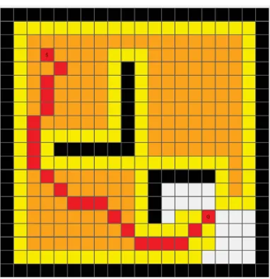
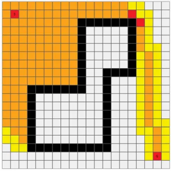
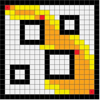
As it is shown in figure 2.29 on page 31: The gray scale demonstrates the magnitude of the artificial potential field, where the lighter cells have smaller magnitudes. The white areas are the potential wells, where the direction of the gradient around the white cells are pointing to it. When the agent is staying in the potential well without enough speed, it cannot escape from the potential well since the force will always push
it back.
Figure 2.29: Magnitude of the APF
combined with the artificial potential field to avoid this trap.
Goal-Non-Reachable-with-Obstacle-Nearby (GNRON) Problem
The Goal-Non-Reachable-with-Obstacle-Nearby problem is another drawback of the
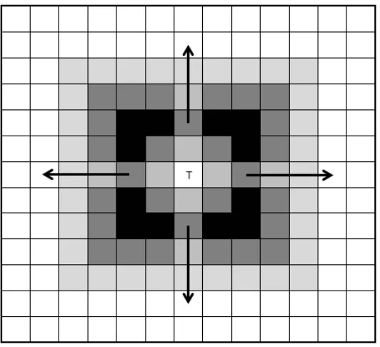
[image:49.612.143.409.253.496.2]artificial potential field [2] [3]: when the target is near an obstacle, the distribution of the gradient around the target has a possibility that it does not point to target but away from it since the magnitude distribution is affected by multiple objects.
Figure 2.30: Target is not reachable due to the obstacles around
The figure 2.30 illustrates a sample of the GNRON problem: although the target in the centre has a smaller magnitude, the cells around it affected by the obstacle have higher magnitude that causes the direction of the gradient around it are point to the outer sides. As the result, when the agent is moving towards this area, it cannot reach the target.
2.2.4 Related Works based on the Artificial Potential Field
Although the artificial potential field is an effective method of robotics navigation, the limitations of the artificial potential field can pose problems. Yang X, Yang W and
2.2. THE ARTIFICIAL POTENTIAL FIELD ALGORITHM 33
time to identify the existence of the potential well, as it cannot figure out all the probable wells on the way. Also, Sun & Han explored the usage of the artificial potential
field for 3D path planning in 2016 [1] by designing a better model. Another research by Liu & Zhao in 2016 [3] uses virtual way-points that contained the concept of search algorithms.
The research by Ge & Cui in 2000 [51] explored an improvement of resolving the GNRON problem of the artificial potential field. By adding an extra factor of torque,
the agent will always take a tangential force near the obstacle, where the centre of the torque is inside the obstacle. This factor allows the agent to move around the obstacle towards the goal. However, the solution didn’t exposed the effects of moving obstacles, as the torques of different obstacle may cancel each other if the distance between the obstacles change. Also, for unknown terrain, the direction of the torque could not be
decided.
The research by Wang & Chirikjian in 2000 [24] illustrates an alternative methodology of using the artificial potential field: by extending the space and involving the z-axis limited to [0,2π), which represents the orientation of the agent and the obstacles. With this extension, the artificial potential field has the ability to resolve the navigation of
an agent as long as it is not in the shape of sphere.
In 2012, Li, Yamashita, Asama, & Tamura demonstrated a solution of using regression search to improve the artificial potential field [5]. In this research, the regression search algorithm is used to keep finding the way-points around the obstacle and uses a methods like line-of-sight to remove the intermediate way-points when the agent is close to the
obstacle.
Another research from Zhejiang University and the University of Tokyo in 2015 explored an improved method of the artificial potential field called SIFORS [25], which is partly involved with search algorithms. Similarly, this algorithm optimizes the path after the path planning by the artificial potential field, by removing the way-points close to the
obstacles with the concept of line-of-sight and keep checking the direction of the current way-point.
The research by Manalu in 2014 [36] illustrates the method of double targets potential field (DTPF). Different from the traditional potential field that has only one target, the DTPF generates the attractive point by using two targets at same time. However,
2.3
Introduction of the Robot Soccer Game
The robot soccer game uses the robots controlled by the artificial intelligence playing
soccer. The general rules of the robot soccer are similar to the normal soccer game. The purpose is to kick the ball on the field into the goal of the opponent, while defensing the attacks from the opponent.
Eslami, Asadi, Soleymani & Azimirad discussed the efficiency of using various algo-rithms for robot path planning in 2014. [52], and exposed that the path-planning and motion control could be manipulated in the grid-based field.
There are two types of the robot in the game: the attacker and the keeper.
During the game, the attacker should have the abilities to pursue the target and avoid the obstacles which could be the opponent robot or the walls. Also, it should be able to kick the ball towards the gate of the opponent.
Different from the attacker, the keeper should have the ability to protect the goal by
various behaviors. Furthermore, when the ball is far away from the goal, it should not keep moving but should park at a certain position waiting for the attacks. It should not be too far away from the goal area.
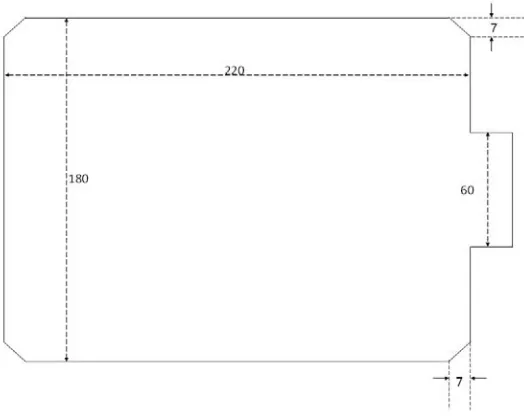
2.3.1 Dimensions of the Playing Field and the Agents
According to the manual of the robot soccer game [22] introduced by Yujin Robotics, Co., Ltd. Korea, 2003, the playing field is rectangle ground with a size of 220×180, and the length of the goals are 60 in the middle of the left and right side. At each corner of the playing field, there is a bevel which angle is 45◦ where the length of short
edges are 7. The figure 2.31 illustrates the overall size of the playing field.