VOLCO: a predictive model for 3D printed microarchitecture

(1)

Contents lists available atScienceDirect

Additive Manufacturing

journal homepage:www.elsevier.com/locate/addma

VOLCO: A predictive model for 3D printed microarchitecture

Andrew Gleadall

a,c,⁎

, Ian Ashcroft

b

, Joel Segal

a

a_{Advanced Manufacturing Technology Research Group, Faculty of Engineering, University of Nottingham, University Park, Nottingham, NG7 2RD, UK} b_{Centre for Additive Manufacturing, Faculty of Engineering, University of Nottingham, University Park, Nottingham, NG7 2RD, UK}

c_{Wolfson School of Mechanical and Manufacturing Engineering, Loughborough University, Loughborough, Leicestershire, LE11 3TU, UK}

A R T I C L E I N F O

Keywords: 3D printing

3D geometry modelling Finite element analysis Voxel model

Tissue engineering scaﬀolds

A B S T R A C T

Material extrusion additive manufacturing is widely used for porous scaffolds in which polymerfilaments are extruded in the form of log-pile structures. These structures are typically designed with the assumption that filaments have a continuous cylindrical profile. However, as afilament is extruded, it interacts with previously printedfilaments (e.g. on lower 3D printed layers) and its geometry varies from the cylindrical form. No models currently exist that can predict this critical variation, which impactsfilament geometry, pore size and me-chanical properties. Therefore, expensive time-consuming trial-and-error approaches to scaffold design are currently necessary. Multiphysics models for material extrusion are extremely computationally-demanding and not feasible for the size-scales involved in scaffold structures.

This paper presents a new computationally-efficient method, called the VOLume COnserving model for 3D printing (VOLCO). The VOLCO model simulates material extrusion during manufacturing and generates a voxelised 3D-geometry-model of the predicted microarchitecture. The extrusion-deposition process is simulated in 3D as afilament that elongates in the direction that the print-head travels. For each simulation step in the model, a set volume of new material is simulated at the end of thefilament. When previously 3D printed filaments obstruct the deposition of this new material, it is deposited into the nearest neighbouring voxels according to a minimum distance criterion. This leads tofilament spreading and widening.

Experimental validation demonstrates the ability of VOLCO to simulate the geometry of 3D printedﬁlaments. In addition,ﬁnite element analysis (FEA) simulations utilising 3D-geometry-models generated by VOLCO de-monstrate its value and applicability for predicting mechanical properties. The presented method enables structures to be validated and optimised prior to manufacture. Potential future adaptations of the model and integration into 3D printing software are discussed.

1. Introduction

The material extrusion additive manufacture of complex structures such as lattices and porous scaffolds is an active researchfield [1,2]. 3D printing of tissue engineering scaffolds has reached a level of maturity where cell-laden hydrogels can be extruded together with biodegrad-able polymers for tissue regeneration in any shape [3,4]. Computer modelling and simulation can be used to enhance and optimise the 3D printing process. In 2009, Mironov et al. [5] identified a need for new computer models in their biofabrication review paper and stated,“We strongly believe that biofabrication from the start must be a predictable technology and built on predictable models and measurable para-meters.”But this issue has still not been addressed since Pati et al. [6], Paulsen and Miller [7] and Tang et al. [8] still highlight a need for mathematical modelling and computer simulations to support the de-sign of tissue engineering constructs. Similarly, a 2017 review of

additive manufacturing of lattice structures [2] identiﬁed several as-pects of 3D printing that require new modelling capabilities.

There is growing interest in the use of computational modelling and simulation for biofabrication [9]. Therefore, porous scaffolds are used for demonstrations in this study. An important application of compu-tational models is to enable validation and optimisation of scaffold microarchitecturea priori, as opposed to through a traditional experi-mental trial-and-error approach. Througha priorioptimisations, Gian-nitelli et al. suggest that“finite element analysis has played a major role in the reduction ofin vitroandin vivoexperimental efforts”[9]. Indeed, a large number of studies have used FEA to validate or optimise scaffold structures including for mechanical properties [10,11], oxygen diff u-sion [12] and cell responses to external loads [13]. A key limitation of the above simulations is that the accuracy strongly depends on the geometric accuracy of the 3D-geometry-model being evaluated. Other complex structures such as lattices also need computational simulation

https://doi.org/10.1016/j.addma.2018.04.004 Received 17 November 2017; Accepted 3 April 2018

⁎_{Corresponding author at: Wolfson School of Mechanical and Manufacturing Engineering, Loughborough University, Loughborough, Leicestershire, LE11 3TU, UK.}

E-mail address:[email protected](A. Gleadall).

Available online 04 April 2018

(2)

of mechanical properties due to the impracticality of iterative experi-mentation in terms of cost and time [2].

At present, discrepancies between the designed 3D geometry and final printed structure are poorly understood [2,9]. For example, in many scaffolds fabricated by material extrusion additive manu-facturing,filaments widen as they cross previously deposited perpen-dicular filaments [14–17]. This impacts the scaffold geometry and mechanical properties but no modelling techniques currently exists that can simulate this geometrical variation. Thus, computational analyses and optimisation of scaffolds prior to 3D printing is currently limited by a lack of accurate predictive geometric modelling techniques. Addi-tional causes of variation to filament geometry include: changes in print-toolpath direction;filament interactions with the build platform; andfilament interactions due to deposition directly on top of existing parallelfilaments. A recent review of additive manufacturing of lattice structures [2] concluded that“geometrical discrepancy [between the designed and manufactured geometry] is a critical issue”and that“the manufacturing influence of additive manufacturing processes cannot be neglected by designers.” They also report that it is“imperative to si-mulate the mechanical properties of lattice structures" and that

“[manufacturing factors] need to be incorporated in to the geometric models.”This clearly indicates the immediate need for new models to predict the microscale geometry of 3D printed structures.

Multiphysics simulations can give highly detailed insights into manufacturing processes. However, the following examples demon-strate the high computational requirements of simulations that consider heat transfer/convection, liquid/solid phase changes and materialﬂow:

•

Even when simplifying the simulation to be 2D, a recent multi-physics study of heat transfer during welding required several days of high performance computing time [18].

•

A 3D welding simulation study [19] required 1–3 days of compu-tation time even with an order of magnitude coarser resolution

(0.2–3.2 mm) than may be required for tissue engineering scaﬀold simulations (note that the number of 3D elements increases with resolution to the power of 3).

•

A recent study for heat transfer in laser-based additive manufacture utilised a resolution of approximately 1 mm [20], over an order of magnitude more coarse than is required to eﬀectively simulate a tissue engineering scaﬀold.

It is unfeasible to use multiphysics models to simulatefilament ex-trusion of 3D printed scaffolds due to the high computational demands. This applies to any structure with geometric features spanning several size-scales. Therefore, a simplified modelling approach is required to enable feasible computational requirements for complex structures.

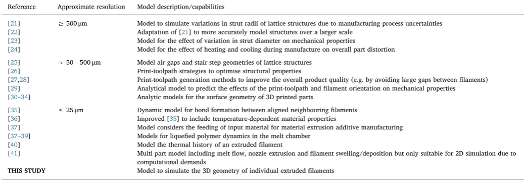
Simpliﬁed models for material extrusion additive manufacturing are reviewed inTable 1, but none can predict the 3D microarchitecture for complex structures with multi-directional interactions between in-dividualﬁlaments:

•

Studies with a resolution > 500μm [21–24] consider geometry variation over a distance of several millimetres to centimetres. They allow useful simulation of large structures, but the variation of 3D geometry for individualﬁlaments is out of scope - their fundamental modelling concepts are, by design, not applicable to individualﬁ -laments.

•

Studies with a resolution of≈50–500μm [25–34] have focused on the print-toolpath [26–29] or analytically modelling the surface of 3D printed parts [30–34]. The geometry of individualfilaments is assumed to be constant along the length of afilament. Therefore, none of the models are designed to simulate interactions between filaments in arbitrary orientations and cannot be translated to do so (due to the fundamental principles of the models, which are ne-cessary for analytical calculations).

•

Studies with afiner resolution (typically≤25μm) [35–41] focus on specific aspects of the material extrusion additive manufacturing process in order to ensure computational feasibility. Models have been developed for dynamic bond formation between parallel fused filaments [35,36], but they are not applicable to tissue engineering scaffolds becausefilaments in scaffolds have non-parallel orienta-tions. Other studies considered individual stages of the material extrusion additive manufacturing process, including the feeding of input material [37], liquefied polymer dynamics in the melt chamber [37–39] and thermal history of an extruded filament [35,40]. Several models were integrated together in the thesis of Bellini [41] to simulate melt flow, nozzle extrusion andfilament swelling/deposition. However, the computation-demands of their Nomenclature

Symbol

ds Simulation step distance (μm) rd Deposition radius (μm) Vd Deposition volume (mm3₎

ve 3D printer extrusion rate (mm3_/mm) lv Voxel side length (μm)

[image:2.595.36.555.566.744.2]

LT Layer thickness (μm)

Table 1

Computational models for material extrusion additive manufacturing.

Reference Approximate resolution Model description/capabilities

[21] ≥500μm Model to simulate variations in strut radii of lattice structures due to manufacturing process uncertainties [22] Adaptation of [21] to more accurately model structures over a larger scale

[23] Model for the eﬀect of variation in strut diameter on mechanical properties

[24] Model for the eﬀect of heating and cooling during manufacture on overall part distortion [25] ≈50 - 500μm Model air gaps and stair-step geometries of lattice structures

[26] Print-toolpath strategies to optimise structural properties

[27,28] Print-toolpath generation methods to improve the overall product quality (e.g. by avoiding large gaps betweenfilaments) [29] Analytical model to predict the effects of the print-toolpath andfilament orientation on mechanical properties [30–34] Analytic models for the surface geometry of 3D printed parts

[35] ≤25μm Dynamic model for bond formation between aligned neighbouringﬁlaments [36] Improved [35] to include temperature-dependent material properties

[37] Model considers the feeding of input material for material extrusion additive manufacturing [37–39] Models for liqueﬁed polymer dynamics in the melt chamber

[40] Model the thermal history of an extrudedﬁlament

[41] Multi-part model including meltﬂow, nozzle extrusion andﬁlament swelling/deposition but only suitable for 2D simulation due to computational demands

(3)

advanced model limited simulations to 2D. Therefore, although their model has high value for research and process development, it is not suitable for use by 3D printer end-users to predict the 3D geometry of a tissue engineering scaﬀold.

This study presents a new VOLume COnserving model for extrusion-based 3D printing (VOLCO). The complex interaction between multiple extruded filaments is modelled based on a simple principle of con-servation of volume. An accurate 3D-geometry-model of the predicted as-fabricated microarchitecture is generated by the model. No other models currently exist to achieve such predictions. The novel predictive model establishes the first step in bridging the gap between multi-physics models (which strive to capture the full range of factors that influence the fundamental 3D printing process) and computer programs currently available to 3D printer end-users (limited or no predictive capabilities). An application of porous scaffolds is used to demonstrate the model capabilities here because the individual extrudedfilaments in

such scaﬀolds have highly variable microscale geometries. The applic-ability of the model to otherﬁelds is discussed.

The structure of the rest of this article is as follows: in the next section, the VOLCO model is described along with the materials and methods used in simulations and experiments; Section3presents the results of experimental validation and demonstrates predictive cap-abilities of the model; and Section4discusses the value, limitations and future opportunities for VOLCO.

2. Materials and methods

2.1. Voxel modelling concept

[image:3.595.84.519.251.704.2]

The concept of the VOLCO model is to simulate the deposition of 3D printedﬁlaments in a virtual 3D voxel environment. The model simu-lates a virtualﬁlament that elongates in the direction that the print head moves in a series of steps (Fig. 1a). The key strength of VOLCO is

(4)

to simulate how the newly 3D printed filament interacts with pre-viously printedfilaments - at present, there are no methods available for the simulation of filament interactions (except continuous linear stacking of parallel filaments). Fundamentally, VOLCO is based on a simple assumption of conservation of volume: if new material deposited at the end of thefilament is blocked by previously depositedfilaments (top part ofFig. 1b), the material is positioned as close as possible to the end of thefilament in the virtual environment according to a minimum distance criterion (bottom part of Fig. 1b). This concept removes the need to consider complex effects of temperature-dependent viscoelas-ticity,fluid mechanics and heat transfer, which would render simula-tions of the size-scales undertaken in this paper computationally-un-feasible. Assumptions and limitations of this fundamental concept are considered in Section2.3and in the discussion. A 3D representation of the voxel modelling concept is shown inFig. 1c, in which afilament is blocked by a previously 3D printedfilament and therefore expands. 2.2. Model parameters

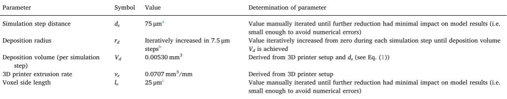
Parameters used in VOLCO are given inTable 2and described in this section. The simulation step distance (ds) is the length of elongation of theﬁlament versus the previous simulation step, as shown inFig. 1a. This is equal to the distanced travelled by the printhead between si-mulation steps. Asdsapproaches zero, the model approaches simulation of continuous extrusion (as opposed to discrete steps). Asdsincreases, computational demands reduce but the value must be set small enough to avoid the introduction of artifacts in the 3D-geometry-model. Prac-tically, to ensure simulation accuracy, the value of thedsparameter is reduced during simulations until further reduction has negligible im-pact on model results. Opportunities for automated recommendation of appropriate parameter values are considered in the discussion.

The deposition volume parameter (Vd) refers to the volume of ma-terial that is deposited by the nozzle during each simulation step, as shown inFig. 1a. For each simulation step, thefilament elongates and occupies new previously-empty voxels. The total volume of newly-oc-cupied voxels must equal the deposition volume (for conservation of volume). In order to identify which volumes are occupied with new material when thefilament elongates, the deposition radius parameter (rd) is used. Any voxels that lie within this radius from the point at the end of thefilament are considered to be occupied by polymer, as shown in Fig. 1(b) and (d). During simulations,rditeratively increases from zero in small steps (step size stated inTable 2), encompassing an ever-increasing number of voxels, until the volume of newly-occupied voxels equals the required deposition volume. This gradually broadening search for new voxels to be occupied by thefilament naturally achieves the modelling concept of positioning newly-deposited material ac-cording to a minimum distance criterion (when previously printedfi -laments obstruct the newfilament).

The value of Vd is directly derived from the 3D printer setup

according to the 3D printer extrusion rate (ve), which indicates the volume of material extruded per millimetre of printhead travel. The calculation ofvedepends on the design of 3D printer and is typically detailed in the printer manual:

•

For printers that are fed material from aﬁlament-reel, the extrusion rate is controlled by setting the rate at which theﬁlament-reel is fed into the melt chamber.

•

For screw-extrusion printers, the extrusion rate is controlled by setting the rate at which the screw mechanism turns.

•

For syringe-based 3D printers with mechanical syringe-piston dis-placement control, the extrusion rate is controlled by setting the rate at which the piston is depressed.

•

For syringe-based 3D printers with pneumatic syringe-piston con-trol, the rate of material extrusion depends on many factors in-cluding needle size and viscosity. Pneumatic-controlled systems are out of scope for VOLCO, although the model can be potentially extended to consider such systems (see Discussion section). Once the rate of material extrusion has been identiﬁed, the de-position volume for each simulation step is simply calculated as the rate of extrusion multiplied by the distance travelled by the nozzle during a simulation step, as given in Eq. (1):

= ×

Vd ve ds (1)

The 3D position of the printhead is derived from the print-toolpath or machine control code (GCODE). The ﬁlament is simulated im-mediately below the nozzle and elongation of theﬁlament follows an identical path to the printhead. Voxels that are blocked by the printer nozzle in each simulation step are not considered for deposition since they are already occupied (by the nozzle). Similarly, no extrusion was permitted in voxels below the build platform.

None of the parameters in VOLCO need to be adjusted toﬁt ex-perimental data. They are all either directly derived from the 3D printer setup or adjusted purely to ensure numerical accuracy of the model. The model was deliberately kept as fundamental and simple as possible here to allow ﬂexible future adaptation; more advanced, enhanced versions of the model are possible as considered in the discussion. A voxel side length (lv) of 25μm was utilised for the simulations in this study, although smaller voxels withlv= 12.5μm were also tested to check that simulation results remained similar, as discussed in Section 3.2.

2.3. Model assumptions

[image:4.595.41.558.612.713.2]

Key simpliﬁcation and assumptions of the modelling concept are described below. They ensure feasible computational demands and avoid the need for experimentally-calibrated parameters. In this study, we present the fundamental, simplest version of the model and

Table 2

Parameters used in the new modelling concept. No parameters were adjusted toﬁt experimental data. All parameters were either directly derived from the 3D printer setup or varied purely for purposes of ensuring computation accuracy and eﬃciency.

Parameter Symbol Value Determination of parameter

Simulation step distance ds 75μma Value manually iterated until further reduction had minimal impact on model results (i.e. small enough to avoid numerical errors)

Deposition radius rd Iteratively increased in 7.5μm stepsb

Value iteratively increased from zero during each simulation step until deposition volume Vdis achieved

Deposition volume (per simulation step)

Vd 0.00530 mm3 Derived from 3D printer setup andds(see Eq. (1))

3D printer extrusion rate ve 0.0707 mm3/mm Derived from 3D printer setup

Voxel side length lv 25μmc Value manually iterated until further reduction had minimal impact on model results (i.e. small enough to avoid numerical errors)

a _{Simulations were repeated with this value changed to 150}_μ_{m (2× increase) to demonstrate the change had little impact on results (Section}_3.1_).

b _{Simulations were repeated with this value changed to 30}_μ_{m (4× increase) to demonstrate the change had little impact on results (Section}_3.1_).

(5)

demonstrate that even the simplest form of the model has value in si-mulating 3D printed structures. Many of the simplifications and as-sumptions listed below may be addressed in extended versions of the model as required for specific 3D printing applications. For example, a more advanced version of the model specifically for pneumatic 3D printing hydrogels at room temperature may include the capability to relate extrusion rate to syringe pressure but has no need for thermal considerations.

Simpliﬁcation and assumptions:

•

Gravity is not considered

○Justification: gravitational forces are low compared to those that can be exerted by the nozzle;filaments on lower layers evidently surpass gravitational forces to prevent scaffold collapse; the results section of this study show several-fold increases in compressive modulus due to filaments interacting with each other, outweighing any minor effects of gravity.

•

Material does notﬂow after it has been positioned in the model

•

Justiﬁcation: this avoids unfeasible computation demands associated

with multiphysics materialﬂow simulations - without this simpliﬁ ca-tion the model may need to simulate temperature, viscoelasticity and phase changes, which have extremely high computational demands.

•

Thermal contraction is not modelled

•

Justification: VOLCO effectively considers all thermal contraction to be completed by the end of each simulation step. Thermal contraction has a minor effect on geometry (several percent) by comparison to filaments obstructing each other (up to 66% change in experimental filament width in Section 3.1); thermal simulations including con-vection have extremely high computational demands.

•

Material is extruded from the nozzle at a constant rate

•

Justiﬁcation: Molten polymer is considered to be an incompressible ﬂuid; mechanically-driven extrusion forces can overcome forces re-sisting polymer extrusion.

•

Obstructed material is relocated according to a minimum distance criterion

•

Justification: An alternative assumption was initially considered wherebyfilaments are represented as a series of cylindrical segments of varying radius. However, such as assumption runs into complications when the printhead changes direction (jagged edges would be simu-lated). The minimum distance criterion was considered to be aflexible fundamental approach.

2.4. Software simulation routine

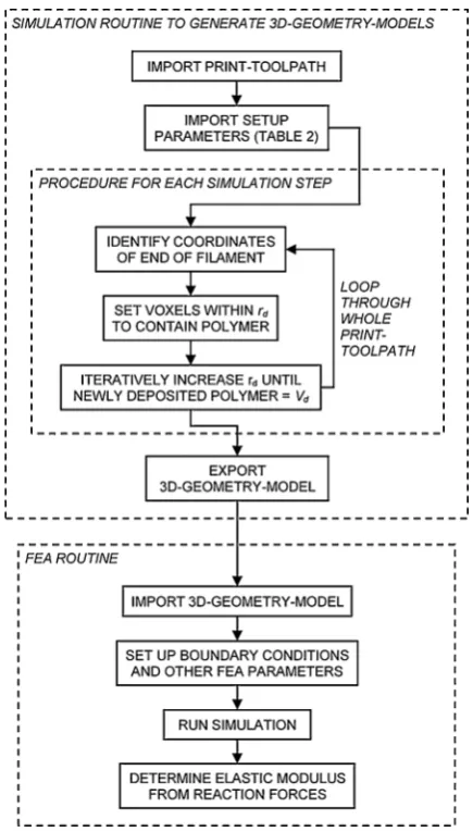
The simulation routine is presented in theﬂowchart inFig. 2. The following steps were followed in MATLAB 2016b to generate 3D-geo-metry-models of the predicted polymer scaﬀold structure:

1 Import a list of printer nozzle coordinates (the print-toolpath) and import the simulation setup parameters inTable 2

2 Identify the Cartesian location of the nozzle, and therefore the di-rection of elongation of theﬁlament, for each simulation step 3 Simulate elongation of the polymerﬁlaments in the voxel 3D matrix

for the print-toolpath. Each simulation step includes the following sub-steps:

a Identify the coordinates considered to be the end of theﬁlament b Setrdto equal the nominalﬁlament radius and set voxels within

this radius to contain polymer

c Determine the increase in the total volume of polymer-voxels in the modelling environment

d If this increase in volume is less thanVd, some of the targeted voxels already contained polymer (e.g. a previous simulatedﬁ -lament). Therefore, iteratively increaserdand set voxels within this radius to contain polymer until the target deposition volume is achieved.

4 Output a 3D-geometry-model of the simulated structure (STLﬁle)

The following steps were taken to model scaﬀold compressive modulus

1 Import the 3D model into the FEA software

2 Setup boundary conditions and other FEA parameters 3 Run simulation

4 Determine compressive modulus from reaction forces

2.5. Experimental scaﬀold design and fabrication

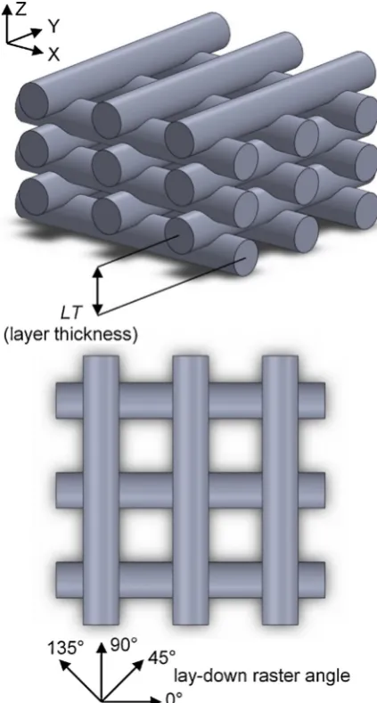
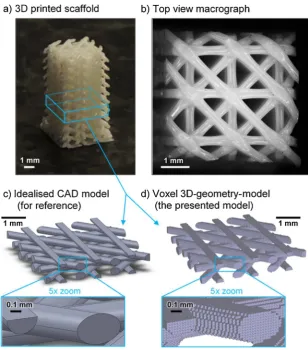
Tissue engineering scaffolds are frequently fabricated by 3D printing layers of polymerfilaments in“log-pile”structures, as shown in the idealised CAD representation inFig. 3. The layer thickness (LT) indicates the vertical distance moved up by the nozzle between layers. It is often varied when 3D printing scaffolds because it can be used to control mechanical properties and porosity. Therefore, in this paper, the model is validated by varying LT and comparing modelled and experimental results for the effects the variation has on compressive modulus,filament geometry and pore fraction.

[image:5.595.323.541.348.731.2]

All scaffolds were 3D printed on an Orion Delta 3D printer in poly lactide (NatureWorks®polylactide 4043D) using a 300μm nozzle dia-meter at a temperature of 210 °C. The rate offilament extrusion was set to achieve a nominal 300μmfilament diameter and the nozzle travel rate was 600 mm min−1. The height of the nozzle above the build platform for thefirst printed layer of all scaffolds was set to 175μm. The 3D printer control code (GCODE) for each scaffold was generated using a custom-developed Visual Basic routine.

(6)

Lay-down patterns of 0/90° and 0/45/90/135° have both been studied in the literature [15,42] and are therefore used to validate the model in this work as detailed inTable 3. To test the effect of layer thickness on pore fraction, 12 mm wide × 12 mm deep × 20-layer scaffolds were 3D printed withLT= 75, 100, and 125μm and a 0/90° lay-down pattern. Small layer thicknesses, in relation to nozzle dia-meter, were used to ensure a high interaction between filaments stacked on top of each other; this forced thefilaments to spread side-ways (to have aflatter, wider cross section as opposed to circular) and therefore provided an effective challenge for the model. To test the effect ofLTon compressive modulus, scaffolds were printed as 18 mm wide × 18 mm deep × 9 mm tall scaffolds withLT= 100, 150, 200 and 250μm and a 0/45/90/135° lay-down pattern. For each printed scaf-fold, nine 4.5 mm × 4.5 mm × 9 mm samples were cut from the central section with a knife blade in a press, using a new blade for each sample.

2.6. Microscopy for porosity andﬁlament width

A Zeiss Stemi 2000-C microscope with a Schott S40-10D ring light was used for microscopy. ImageJ 1.49v (National Institutes of Health)

was used to analyse pore fraction andfilament width.Filament width refers to the width of afilament from a top-down view and must in-crease whenfilaments are more closely stacked on top of each other because thefilaments are impeded from taking a cylindrical form and must spread and widen due to interactions withfilaments on lower layers. This is discussed in more detail in Section3.1. To determine pore fraction, images with a pixel size of 5.4μm were binarised according to greyscale value (0–255) using a threshold of 105. The four central in-ternal pores were analysed for each scaffold to determine average vo-lume fraction. Filament width was measured from the microscope images, midway between crossover points with perpendicular fi la-ments. Fourfilament width measurements were taken for each scaffold.

2.7. Mechanical compression testing

Compressive tests were conducted on an Instron 5969 machine with a 5 kN load cell according to ASTM standard D695. Unconstrained samples were compressed between two steel plates at a rate of 1 mm min−1_{to 50% strain. Five samples (4.5 mm × 4.5 mm × 9 mm)} were tested for each layer thickness. Scaﬀolds were compressed in the build-direction and the initial linear-elastic compression phase was used to calculate compressive modulus.

2.8. Finite element analysis

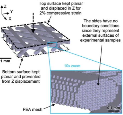
Linear elastic FEA simulations were completed using the commer-cial software package ABAQUS/CAE 6.12-3 (Dassault Systèmes).Fig. 4 shows the mesh and boundary conditions, which were as follows: the lower surface of the 3D model was kept planar and prevented from z-displacement; the top surface of the 3D model was kept planar and a negative z-displacement was applied to achieve 2% strain; the sides of the model were not constrained since they directly represent the un-constrained external surface of the experimental sample. Compressive modulus was calculated based on the z-reaction forces and unit cell area. The elastic modulus parameter was set to 2.45 GPa, which was determined through calibration with the experimental sample forLT = 250μm, as discussed in the results section. This value is reasonable in comparison to values in the literature that range from < 1 GPa to > 7 GPa [43–47]. This single calibrated value was used in simula-tions for all values ofLT. Poisson’s ratio was set to 0.36 [48,49].

2.9. Statistical analysis

Plots for porosity,ﬁlament width and compressive modulus display mean values and error bars indicate standard deviation. Mean percen-tage error (MPE) is calculated according to Eq. (2) as

∑

−

= n

a f

a

100%

t n

t t

t

1 (2)

[image:6.595.55.267.56.451.2]

in whichatis the experimental measurement,ftis the model prediction andnis the number of samples.

Fig. 3.CAD representation of the idealised log-pile structure illustrates a 0°/90° lay-down pattern and the LTparameter that was varied in scaffolds for ex-perimental validation of the model. Note that in this idealised representation, interactions between filaments (e.g.filament spreading/bulging) are not in-dicated - the lack of any existing method to predict such interactions gives justification to and highlights the importance of the presented model.

Table 3

Scaﬀold designs used for validation of the model in this study.

Validation purpose Lay-down pattern

LT(μm) Sample size

Validate ability of model to simulate pore fraction and

ﬁlament spreading

0/90° 75 12 mm wide × 12 mm

deep × 20 layers 100

125

Validate ability of model to support mechanical properties prediction

0/45/90/ 135°

100 4.5 mm × 4.5 mm × 9 mm 150

[image:6.595.307.560.630.746.2]

(7)

3. Results

The results are split into two sections. Thefirst section validates the ability of VOLCO to simulate a scaffold in which 3D printedfilaments are obstructed by previously printedfilaments on lower layers. Due to this obstruction,filaments become wider andflatter. For validation, the 3D-geometry-models generated by VOLCO are compared to experi-mental results. The second section demonstrates the ability of VOLCO to support the prediction of scaffold mechanical properties. The 3D-geometry-models generated by VOLCO are imported into FEA software and used to predict compressive modulus. Experimental samples are 3D printed and tested in order to validate the FEA predictions.

3.1. Modellingﬁlament geometry

Twenty-layer scaffolds with square pores from top-to-bottom were 3D printed (Fig. 5a) to test the ability of the VOLCO modelling concept to simulate the 3D geometry (Fig. 5b). Three different printing setups were used in whichLT= 75, 100 and 125μm. The top-view“ Experi-mental macrograph”images in Fig. 5c show thatfilaments widened (indicated by the arrows to either side of hashed regions) as layer thickness reduced from left to right in thefigure. This widening was due tofilaments being obstructed by previously-printedfilaments (on lower layers) as shown in the idealised schematic at the top ofFig. 5c. AsLT reduced, thefilaments were more obstructed and therefore widened to a greater degree. The VOLCO model effectively captured this trend, as can be seen in the top-view images of 3D-geometry-models at the bottom ofFig. 5c. Filament width was measured from the experimental and model images and the results are given inFig. 6a. The mean per-centage error between the model predictions and experimental values was 5.0% (3 sets of n = 4). This is a good level of predictive accuracy given that experimentalfilament width increased by 66%, from 305 to 505μm experimentally, as LT reduced from 125 to 75μm. For the sample withLT= 75μm,filaments were≈505μm wide by 150μm tall (150μm = 2 × 75μm layer thickness because stacked filaments had the same orientation every two layers, as shown in Fig. 3), which highlights the ability of VOLCO to simulatefilaments with a non-cir-cular cross-section.

Fig. 6b shows the pore fraction measured experimentally (65.2%–77.0%) and from modelling results (68.9%–79.1%). The model simulated the trend effectively but predicted a slightly greater pore fraction for all samples (MPE = 4.6%; 3 sets of n = 4). This may have been due to experimental variation between 3D printed layers: any misalignment betweenfilaments on different layers reduced the visible pore area in top-view images.

[image:7.595.57.272.54.255.2]

Model simulations of 12 mm × 12 mm × 20-layer (1–3 mm) scaf-folds in this section took 20–50 min on a desktop computer. Adjustment Fig. 4.The mesh and boundary conditions used in FEA simulations.

[image:7.595.81.518.424.697.2]

(8)

of model parameters (ds= 150μm instead of 75μm,rd= 30μm instead of 75μm) reduced simulation times to 3–7 min whilst achieving por-osity predictions within 0.2–2.7% of the original values.

3.2. Compressive modulus prediction

This section validates the ability of VOLCO to support FEA simu-lations of scaffold compressive modulus. Four different scaffolds were 3D printed withLT= 100, 150, 200 and 250μm and tested for com-pressive modulus. The sample shown in Fig. 7(a) and (b) had LT= 200μm. VOLCO was used to general 3D-geometry-models of the scaffolds (Fig. 7d). These 3D models were compared to the experi-mental scaffold geometries and were used in FEA simulations to predict compressive moduli. The predicted and experimental values of com-pressive moduli were compared in order to validate the model. To demonstrate the value of the VOLCO model, FEA simulations were also conducted using an idealised CAD model of the scaffold, in whichfi -laments had a constant diameter equal to the nozzle diameter (Fig. 7c) -this is a simple approach that researchers can currently use to generate 3D models of a scaffolds in standard 3D CAD packages. The key dif-ference between the VOLCO model geometries and the idealised CAD model geometries was that the idealised CAD models did not and could not have the scope to considerfilament widening due to obstruction by previously printedfilaments.

3.2.1. Experimental results

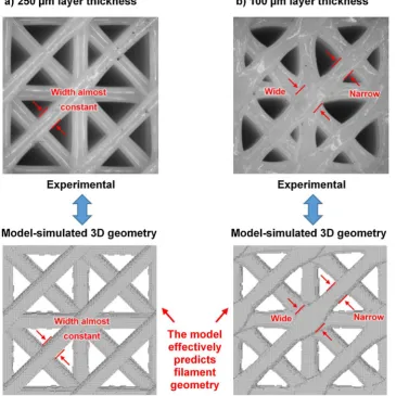
Fig. 8a shows that filaments had a constant diameter in the ex-perimental sample withLT= 250μm. This indicates that thefilaments were not greatly obstructed by otherfilaments (on lower layers), which is expected because the nozzle raised by 250μm between layers: only

50μm less than the nominalfilament diameter (300μm). In contrast, in the sample withLT= 100μm, the nozzle only raised by 33% of the nominalfilament diameter between layers and therefore thefilaments were obstructed and widened at cross-over points with lower-layerfi -laments, as can be seen in Fig. 8b. The widening of filaments at crossover points resulted in compressive modulus increasing more than 5.5× as layer thickness reduced from 250 to 100μm, as shown inFig. 9 (black triangles). The scatter of the individual experimental results (n = 5) was < ± 8% for the samples with LT = 150–250μm and ±

20.5% for the 100μm samples.

3.2.2. Proposed model FEA results

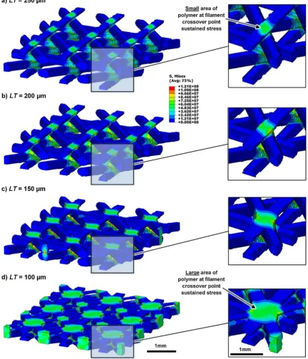
[image:8.595.40.428.54.410.2]

(9)

stress (as can be seen in theFig. 10). AsLTreduced,ﬁlaments widened to a greater degree at crossover points (visible inFigs. 8b andFigure 10) and therefore compressive modulus increased because a wider column of polymer resisted compression compared to samples with a larger layer thickness.

The bulk material elastic modulus parameter in FEA simulations was calibrated to the sample withLT= 250μm because the value is highly dependent on experimental factors such as testing strain rate, stress-strain-curve analysis procedure, polymer molecular weight, compressive versus tensile testing, and many other factors. A calibrated elastic modulus value of 2.45 GPa, which is reasonable for poly lactide [43–47], was used in all four FEA simulations. Even with the FEA ca-libration step, the experimental results present a fair and diﬃcult challenge for the model since there was a large 5.5x increase in ex-perimental compressive modulus for samples with 100μm versus 250μm layer thickness. This change was accurately predicted in the FEA simulations as 5.9× (MPE = 6.6%; n = 5). The mean percentage error versus experimental compressive modulus for all samples was 11% (3 sets of n = 5; 250μm sample was excluded since it was used for calibration).

3.2.3. Idealised CAD model FEA results

Four idealised CAD models were generated in SolidWorks 2016 for the four differentLTvalues and used in FEA simulations for comparison to the VOLCO model. In contrast to 3D-geometry-models generated by the VOLCO model, the idealised CAD models did not consider the ef-fects offilaments widening, therefore FEA predictions obtained using them (Fig. 9hollow circles) did not effectively capture the experimental trend of increasing compressive modulus as layer thickness reduced (Fig. 9 solid black triangles). The mean percentage error versus ex-perimental compressive modulus for all samples was 42.9% (3 sets of

n = 5; 250μm sample was excluded since it was used for calibration). These results highlight the importance of the VOLCO modelling concept being able to simulate ﬁlaments with varying cross-sectional geome-tries. The calibrated elastic modulus value used in FEA for all idealised CAD models was 2.64 GPa.

Each voxel simulation of polymer deposition took less than 5 min and each FEA simulation less than 10 min on a desktop computer. FEA simulations were repeated with a smaller unit cell (one ninth of the size) and planar boundary conditions in the X and Y directions. These simulation results remained within 0.2%–2.8% of those for the original unit cell whilst simulations took just 1 min. Additionally, to test the sensitivity of the model, the voxel side length was halved to lv= 12.5μm. The simulations took an order of magnitude longer but the change had little impact on compressive modulus (< 1% change).

4. Discussion

4.1. Validated capabilities of the VOLCO model

[image:9.595.38.347.52.403.2]

(10)

VOLCO means it can simulate a large range offilament geometries and therefore has applicability to a wide range of different structures: it is demonstrated for log-pile structures but is anticipated to be applicable to other types, such as commonly 3D printed shell + infill parts. The authors are unaware of any models or any previous publications

presenting methods to simulate the varying geometry of individual 3D printedfilaments (aside from models for simple interactions between isolatedfilaments, which have vastly different scope and relevance in comparison to the method presented in this study for full 3D printed structures).

[image:10.595.117.483.60.426.2]

The FEA simulation results demonstrate the value of the 3D-geo-metry-models generated by VOLCO. These 3D-geo3D-geo-metry-models are predictions of the as-fabricated 3D printed microarchitecture. In the present study, these models were used in FEA simulations to predict compressive modulus of the scaffolds. However, the 3D-geometry-models could be used for a wide range of other simulations or analyses, for example to simulate fluid flow or molecular diffusion through a scaffold or to analyse the distribution of pores within the scaffold. By changing the layer thickness of the 3D printed scaffold, compressive modulus was shown to increase 5.5x for experimental samples. The VOLCO model simulated an increase of 5.9x through FEA, which de-monstrates a remarkably accurate prediction for such a large change in compressive modulus with no calibration or fitting of any model parameters (the calibration of the elastic modulus FEA parameter in Section3.2.2bears no impact on these 5.5× and 5.9× increases since they are relative increases). No other models exist that can predict the relationship between compressive modulus and layer thickness de-monstrated here. The results for a simple CAD representation of the structure, which did not account forfilament widening, show that it could not capture the experimental trends. This highlights the im-portance of VOLCO’s ability to simulate variation in filament cross-Fig. 8.(a) The VOLCO model correctly simulatedfilaments to have a constant width in the scaffold withLT= 250μm; and (b) the VOLCO model correctly simulated filaments to widen at cross-over points with lower-layerfilaments in the scaffold withLT= 100μm. The widening resulted from thefilaments being printed closer together (lower layer thickness) and therefore being more obstructed byfilaments on lower layers.

[image:10.595.52.273.476.599.2]

(11)

section. Although layer thickness was varied in this study to validate the model, it could also simulate a wide range of other factors that have been studied experimentally including nozzle size,ﬁlament spacing and lay down pattern.

4.2. Computational demands and 3D printing software integration

The modelling simulations in this study took 3–50 min. Simulations with greater interactions betweenﬁlaments (smaller layer thicknesses) took longer because a greater number of iterations (increasingrd) were required in each simulation step to achieve widerﬁlaments. The au-thors anticipate that simulation times could be reduced to under a

minute with program optimisations for speed. If the method was adapted to consider a periodic unit cell (particularly relevant given the repeating nature of many 3D printed scaﬀolds/lattices), it is likely that eﬀectively-instantaneous predictions of 3D-geometry could be in-tegrated into 3D printer software.

[image:11.595.81.514.60.565.2]

(12)

excessiveﬁlament overlapping. Furthermore, automated predictions of pore size, pore fraction and mechanical properties could be generated (some FEA simulations took < 1 min in the present study).

As an alternative to presenting designers with modelling results, VOLCO could be implemented within 3D printer software to auto-matically optimise the print-toolpath or print parameters. To achieve this, feedback of the model results within the 3D printer program would be utilised to iteratively update the printing setup. In such an approach, the user may specify design requirements (e.g. pore size, compressive modulus, pore fraction) as opposed to printer setup parameters (e.g. extrusion temperature,ﬁlament spacing, layer thickness).

Although some model parameters were iteratively adjusted in this study to ensure numerical accuracy and avoid model artefacts, it would be possible to develop algorithms for automatic identification of model parameters. Preliminary assessment of the print-toolpath and 3D printer setup would determine the model size, the level of interaction between filaments and the extent of filament widening. This would enable software to identify effective parameter values and present the user with a choice of simulation accuracies and respective simulation time estimates.

Lattice generation software can automatically create a 3D lattice structure optimised for requirements such as mechanical properties [50]. The software generates a 3D-geometry-model of the intended structure, which is imported into 3D printing software for print-tool-path generation. During generation of the print-toolprint-tool-path and during fabrication, discrepancies between the intended geometry and thefinal 3D printed geometry are introduced. VOLCO could be integrated into lattice generation software to optimise thefinal fabricated lattice geo-metry, rather than the conceptual 3D geometry. Park and Rosen [25] recently proposed a method to simulate as-fabricated lattice geometries predicted for theoretical designs. Significant improvements in predic-tions for mechanical properties were achieved which demonstrates the importance of modelling discrepancies between designed and manu-factured 3D geometries. In their method, filaments were assumed to have a constant elliptic-rectangular cross section. Therefore, it is a completely different concept to VOLCO and cannot replicate results in the present study because, similar to the idealised CAD model in Section 3.2.3, it does not consider geometric variation of individualfilaments. 4.3. Model limitations and potential extension

The VOLCO model is based on a simple assumption that as afi la-ment is 3D printed, the rate of material deposition remains constant. In other words, if filament extrusion is partly obstructed by previously printed filaments, material is still extruded from the nozzle. In the model, the newly extruded material for each simulation step is posi-tioned according to a minimum distance criterion from a point at the end of the growingfilament. This geometric modelling concept is in-tended to be as fundamental and simple as possible; it allows for a wide range of future adaptations. The modelling concept can be readily ex-tended to consider extra factors for specific deposition conditions or for more detailed analysis. For example: gravitational effects may be added for scaffolds wherefilaments bridge large gaps; process imperfections may be considered such as fluctuations in deposition rate or nozzle position; and melt flow or cooling effects could be incorporated for microstructure analysis.

In many cases, extensions to VOLCO would have negligible impact on computational demands; for example, to simulate the effect of ex-perimentalfluctuations in deposition rate or nozzle position. In terms of implementation, many extensions would require very little repro-gramming of the physical software code; for example, to consider a random misalignment error for each layer, just a single extra line of program code would be required to offset the coordinate list for each new layer.

A limitation of VOLCO is that the extrusion rate of material was considered to be constant, which makes the model applicable for 3D

printers with a mechanically-driven syringe-plungers (e.g. 3DYNAMIC SYSTEMS OMEGA) or screw-extruders (e.g. RegenHU 3DDiscovery), or 3D printers fed by a polymer ﬁlament reel (e.g. REGEMAT3D). For pneumatic printers (e.g. BioBots), it would be interesting to extend the model to include a term to represent pressure in the syringe and relate it to a varying extrusion rate of new material. It may be possible to achieve such an extension with minor increases in computation-de-mands.

Practically, it may be useful to use VOLCO in two phases: 1) un-calibrated - for quick analyses of scaffold geometries and the relative effects of design choices on factors such as compressive modulus; 2) calibrated - (e.g. elastic modulus FEA parameter calibration) for pre-dictive use with a higher level of confidence or to optimise a design for specific requirements.

4.4. Applicability to tissue engineering

For tissue engineering scaffolds, porosity has been shown to be an important factor for cell ingrowth [51], vascularisation [52], nutrient and oxygen exchange [12], and mechanical properties [14]. The ability to predict pore size and pore fraction enables scaffold designs and printer settings to be optimised for desired characteristics with reduced experimental trials. It addresses the gap that currently exists between designed and manufactured scaffold microarchitectures and improves the link between experimental and computational models that is cur-rently lacking [7,9].

As discussed above, two key potential uses of the model are as follows:

•

Validation and optimisation of a scaﬀold design prior to printing

•

Automated optimisation of printer parameters and the

print-tool-path through feedback of model results within 3D printer software Validation of a scaffold design prior to printing enables better de-sign optimisation during the dede-sign process and is therefore hugely beneficial to reduce experimental iteration [6,7]. Currently, char-acterisation of scaffold design is often achieved through 3D printing > microCT scanning > microCT 3D-geometry-model gen-eration > microCT 3D-geometry-model analyses. This is a time-con-suming process that requires several days of expensive resources. In contrast, the VOLCO model can be useda priorito optimise or validate a construct design in a few minutes. Althoughfinal scaffold geometries should still be characterised experimentally, the use of the model may save days or weeks of trial-and-error printing. Furthermore, the 3D-geometry-models generated by VOLCO enable a very wide range of potential analyses including pore fraction, pore shape/size, open/closed porosity, oxygen diffusion, mechanical properties and computational fluid dynamics. Future work could also translate the model to bioma-terials including cell-laden hydrogels.

In situations where scaffold designs must be optimised for several factors (e.g. mechanical properties, degradation profile and biological response), the number of experiments required for trial-and-error op-timisation may be impractical. New design strategies to determine the optimal trade-offbetween the conflicting requirements are necessary [9]. The 3D geometry predictions of the VOLCO model may enable topological optimisation of multiple parameters due to low computa-tional demands. The improved predictions achieved by the model may enable more accurate computational modelling of biomechanical forces in cells or biological responses, and thus support important efforts to reduce the number of animals required forin vivostudies [8].

(13)

4.5. Applicability outside of tissue engineering

Although this study demonstrated VOLCO for tissue engineering scaffolds, it is potentially suitable to a wide range of 3D printing ap-plications. For most 3D printed parts,filaments are printed closer to-gether than in log-pile tissue engineering scaffolds. The validation re-sults in Section3.1show that the modelling concept can simulate the geometry offilaments that are closely stacked. Even coarse simulations with very low computational demands (e.g. a large voxel side length of lv= 50μm) could prove highly useful in previewing parts prior to printing. In the authors’opinion, such simulations could potentially be conducted in less time than that taken by print-toolpath generation algorithms. Many aspects discussed in relation to tissue engineering above directly translate to other applications; for example where infill is used, the new modelling concept could enable the user to specify infill mechanical properties rather than infill density. Furthermore, the model may be translated to other processes; particularly those based on volumetric deposition such as inkjet 3D printing, for which the geo-metry of each droplet would be simulated.

5. Conclusions

This paper presented a new modelling technique, called VOLCO, to predict the microarchitecture of tissue engineering scaffolds by con-sidering interactions between 3D printed filaments. It simulatedfi la-ments being 3D printed and generated 3D-geometry-models of the predicted structures. The voxel-based technique successfully simulated filament geometries ranging from nominally circular cross-sections (300μm diameter) to wideflat cross-sections (505μm wide × 150μm tall). Filament width and pore fraction were predicted with mean per-centage errors of 5.0% and 4.6%, respectively. It was also shown that the 3D-geometry-models generated by the VOLCO model can be used to predict compressive modulus through FEA simulations. During valida-tion experiments, compressive modulus was found to increase 5.5 fold experimentally as the 3D printer layer thickness reduced from 250 to 100μm. VOLCO predicted this increase to be 5.9 fold, which is ex-tremely accurate for such a large modulus range and given that the prediction was achieved with nofitting of any model parameters. No other models or methods have been reported that can generate such predictions.

VOLCO has low computation demands. Generation of 3D-geometry-models that were used in FEA simulations took less than 5 min. For the repeating structures often used in tissue engineering scaﬀolds, eﬀ ec-tively-instantaneous predictions are a realistic prospect if a repeating unit cell were utilised in simulations. The model is therefore highly suited for integration into 3D printer software, both for tissue en-gineering and potentially more general 3D printing applications.

The new modelling technique is a powerful tool that can be used to validate the geometry and properties of tissue engineering scaffolds before manufacture. It is hoped that it forms the foundation for a wide range of future adaptations that extend modelling capabilities for more detailed, application-specific analyses. Further research into computa-tional modelling and simulation is critical to support future advance-ment of the 3D printingfield, in particular to further understand or predict the as-fabricated structure and properties of 3D printed con-structs.

Acknowledgments

The research leading to these results has received funding from the EPSRC [grant number EP/H028277/1] in the EPSRC Centre for Innovative Manufacturing in Regenerative Medicine. The MATLAB si-mulation routine developed in this study implemented the CONVERT_voxels_to_stl script written by Adam. H. Aitkenhead [53].

Supplementary data

Research data for experimental compression tests are available from the institutional data repository of Loughborough University [54]. Other data and models can be requested from the corresponding author. References

[1] I.T. Ozbolat, M. Hospodiuk, Current advances and future perspectives in extrusion-based bioprinting, Biomaterials 76 (2016) 321–343.

[2] G. Dong, Y. Tang, Y.F. Zhao, A survey of modeling of lattice structures fabricated by additive manufacturing, J. Mech. Des. 139 (10) (2017).

[3] H.-W. Kang, S.J. Lee, I.K. Ko, C. Kengla, J.J. Yoo, A. Atala, A 3D bioprinting system to produce human-scale tissue constructs with structural integrity, Nat. Biotechnol. 34 (3) (2016) 312–319.

[4] L. Jung-Seob, H. Jung Min, J. Jin Woo, S. Jin-Hyung, O. Jeong-Hoon, C. Dong-Woo, 3D printing of composite tissue with complex shape applied to ear regeneration, Biofabrication 6 (2) (2014).

[5] V. Mironov, T. Trusk, V. Kasyanov, S. Little, R. Swaja, R. Markwald, Biofabrication: a 21st century manufacturing paradigm, Biofabrication 1 (2) (2009) 1–16. [6] F. Pati, J. Jang, J.W. Lee, D.-W. Cho, Chapter 7 - extrusion bioprinting, in: A. Atala,

J.J. Yoo (Eds.), Essentials of 3D Biofabrication and Translation, Academic Press, Boston, 2015pp. 123-152.

[7] S. Paulsen, J. Miller, Tissue vascularization through 3D printing: will technology bring usﬂow? Dev. Dyn. 244 (5) (2015) 629–640.

[8] D. Tang, R.S. Tare, L.-Y. Yang, D.F. Williams, K.-L. Ou, R.O.C. Oreﬀo, Biofabrication of bone tissue: approaches, challenges and translation for bone regeneration, Biomaterials 83 (2016) 363–382.

[9] S.M. Giannitelli, D. Accoto, M. Trombetta, A. Rainer, Current trends in the design of scaﬀolds for computer-aided tissue engineering, Acta Biomater. 10 (2) (2014) 580–594.

[10] S. Eshraghi, S. Das, Mechanical and microstructural properties of polycaprolactone scaﬀolds with one-dimensional, two-dimensional, and three-dimensional ortho-gonally oriented porous architectures produced by selective laser sintering, Acta Biomater. 6 (7) (2010) 2467–2476.

[11] H.A. Almeida, P.J. Bártolo, Numerical simulations of bioextruded polymer scaﬀolds for tissue engineering applications, Polym. Int. 62 (11) (2013) 1544–1552. [12] J. Woo Jung, H.-G. Yi, T.-Y. Kang, W.-J. Yong, S. Jin, W.-S. Yun, D.-W. Cho,

Evaluation of the effective diffusivity of a freeform fabricated scaffold using com-putational simulation, J. Biomech. Eng. 135 (8) (2013) 1–7.

[13] K. Chang Yan, K. Nair, W. Sun, Three dimensional multi-scale modelling and ana-lysis of cell damage in cell-encapsulated alginate constructs, J. Biomech. 43 (6) (2010) 1031–1038.

[14] I. Zein, D.W. Hutmacher, K.C. Tan, S.H. Teoh, Fused deposition modeling of novel scaﬀold architectures for tissue engineering applications, Biomaterials 23 (4) (2002) 1169–1185.

[15] B.C. Tellis, J.A. Szivek, C.L. Bliss, D.S. Margolis, R.K. Vaidyanathan, P. Calvert, Trabecular scaﬀolds created using micro CT guided fused deposition modeling, Mater. Sci. Eng. C 28 (1) (2008) 171–178.

[16] M. Domingos, F. Chiellini, A. Gloria, L. Ambrosio, P. Bartolo, E. Chiellini, Eﬀect of process parameters on the morphological and mechanical properties of 3D bioex-truded poly(ε-caprolactone) scaﬀolds, Rapid Prototyp. J. 18 (1) (2012) 56–67. [17] J.E. Trachtenberg, P.M. Mountziaris, J.S. Miller, M. Wettergreen, F.K. Kasper,

A.G. Mikos, Open-source three-dimensional printing of biodegradable polymer scaﬀolds for tissue engineering, J. Biomed. Mater. Res. A (2014) 1–10. [18] M. Dal, P. Le Masson, M. Carin, A model comparison to predict heat transfer during

spot GTA welding, Int. J. Therm. Sci. 75 (2014) 54–64.

[19] W.-I. Cho, S.-J. Na, C. Thomy, F. Vollertsen, Numerical simulation of molten pool dynamics in high power disk laser welding, J. Mater. Process. Technol. 212 (1) (2012) 262–275.

[20] P. Michaleris, Modeling metal deposition in heat transfer analyses of additive manufacturing processes, Finite Elem. Anal. Des. 86 (2014) 51–60.

[21] S.-I. Park, D.W. Rosen, S.-K. Choi, C.E. Duty, Eﬀective mechanical properties of lattice material fabricated by material extrusion additive manufacturing, Addit. Manuf. 1–4 (0) (2014) 12–23.

[22] R.M. Gorguluarslan, S.-I. Park, D. Rosen, S.-K. Choi, A multilevel upscaling method for material characterization of additively manufactured part under uncertainties, J. Mech. Des. 137 (11) (2015) 1–12.

[23] M.R. Ravari, M. Kadkhodaei, M. Badrossamay, R. Rezaei, Numerical investigation on mechanical properties of cellular lattice structures fabricated by fused deposition modeling, Int. J. Mech. Sci. 88 (0) (2014) 154–161.

[24] Y. Zhang, K. Chou, A parametric study of part distortions in fused deposition modelling using three-dimensionalﬁnite element analysis, Proceedings of the Institution of Mechanical Engineers, Part B: Journal of Engineering Manufacture vol. 222, (8) (2008) 959–968.

[25] S.-i. Park, D.W. Rosen, Quantifying eﬀects of material extrusion additive manu-facturing process on mechanical properties of lattice structures using as-fabricated voxel modeling, Addit. Manuf. 12 (2016) 265–273.

[26] P. Kulkarni, D. Dutta, Deposition strategies and resulting part stiﬀnesses in fused deposition modeling, J. Manuf. Sci. Eng. 121 (1) (1999) 93–103.

(14)

for material extrusion-based additive manufacturing technology, Addit. Manuf. 1–4 (2014) 32–47.

[29] D. Croccolo, M. De Agostinis, G. Olmi, Experimental characterization and analytical modelling of the mechanical behaviour of fused deposition processed parts made of ABS-M30, Comp. Mater. Sci. 79 (2013) 506–518.

[30] P.M. Pandey, K. Thrimurthulu, N.V. Reddy, Optimal part deposition orientation in FDM by using a multicriteria genetic algorithm, Int. J. Prod. Res. 42 (19) (2004) 4069–4089.

[31] R.I. Campbell, M. Martorelli, H.S. Lee, Surface roughness visualisation for rapid prototyping models, Comput. Aided Des. 34 (10) (2002) 717–725.

[32] A. Mason, Multi-Axis Hybrid Rapid Prototyping Using Fusion Deposition Modeling, Ryerson University, Canada, 2006.

[33] H.S. Byun, K.H. Lee, Determination of optimal build direction in rapid prototyping with variable slicing, Int. J. Adv. Manuf. Technol. 28 (3–4) (2006) 307–313. [34] D.-K. Ahn, S.-M. Kwon, S.-H. Lee, Expression for surface roughness distribution of

FDM processed parts, International Conference on Smart Manufacturing Application, Korea, 2008 pp. 490-493.

[35] C. Bellehumeur, L. Li, Q. Sun, P. Gu, Modeling of bond formation between polymer

ﬁlaments in the fused deposition modeling process, J. Manuf. Process. 6 (2) (2004) 170–178.

[36] B. Graybill, Development of a Predictive Model for the Design of Parts Fabricated by Fused Deposition Modeling, University of Missouri, Columbia, 2010.

[37] A. Bellini, S. Guceri, M. Bertoldi, Liqueﬁer dynamics in fused deposition, J. Manuf. Sci. Eng. 126 (2) (2004) 237–246.

[38] H.S. Ramanath, C.K. Chua, K.F. Leong, K.D. Shah, Meltﬂow behaviour of poly-ε -caprolactone in fused deposition modelling, J. Mater. Sci. Mater. Med. 19 (7) (2008) 2541–2550.

[39] N. Sa’ude, M. Ibrahim, M.H.I. Ibrahim, Meltﬂow behavior of polymer matrix ex-trusion for Fused Deposition Modeling (FDM, Appl. Mech. Mater. 660 (2014) 89–93.

[40] Q. Sun, G. Rizvi, C. Bellehumeur, P. Gu, Eﬀect of processing conditions on the bonding quality of FDM polymerﬁlaments, Rapid Prototyp. J. 14 (2) (2008) 72–80. [41] A. Bellini, Fused Deposition of Ceramics: A Comprehensive Experimental,

Analytical and Computational Study of Material Behavior, Fabrication Process and Equipment Design, Drexel University, USA, 2002.

[42] M. Domingos, F. Chiellini, S. Cometa, E. De Giglio, E. Grillo-Fernandes, P. Bartolo, E. Chiellini, Evaluation of in vitro degradation of PCL scaﬀolds fabricated via BioExtrusion. Part 2: inﬂuence of pore size and geometry, Virtual Phys.Prototyp. 6

(3) (2011) 157–165.

[43] E.M. James, Polymer Data Handbook, Oxford University Press, New York, 1999 p. 631.

[44] J.S. Bergström, D. Hayman, An overview of mechanical properties and material modeling of polylactide (PLA) for medical applications, Ann. Biomed. Eng. 44 (2) (2016) 330–340.

[45] D.J. Hickey, B. Ercan, L. Sun, T.J. Webster, Adding MgO nanoparticles to hydroxyapatite–PLLA nanocomposites for improved bone tissue engineering ap-plications, Acta Biomater. 14 (2015) 175–184.

[46] S.-l. Yang, Z.-H. Wu, W. Yang, M.-B. Yang, Thermal and mechanical properties of chemical crosslinked polylactide (PLA), Polym. Test. 27 (8) (2008) 957–963. [47] I. Armentano, M. Dottori, E. Fortunati, S. Mattioli, J. Kenny, Biodegradable polymer

matrix nanocomposites for tissue engineering: a review, Polym. Degrad. Stab. 95 (11) (2010) 2126–2146.

[48] X. Li, C. Guo, X. Liu, L. Liu, J. Bai, F. Xue, P. Lin, C. Chu, Impact behaviors of poly-lactic acid based biocomposite reinforced with unidirectional high-strength mag-nesium alloy wires, Prog. Nat. Sci. Mater. Int. 24 (5) (2014) 472–478. [49] J. Lai, Moldﬂow Material Testing Report MAT2238 NatureWorks PLA, (2007) pp.

1-34.

[50] A. Aremu, J. Brennan-Craddock, A. Panesar, I. Ashcroft, R.J. Hague, R.D. Wildman, C. Tuck, A voxel-based method of constructing and skinning conformal and func-tionally graded lattice structures suitable for additive manufacturing, Addit. Manuf. 13 (2017) 1–13.

[51] C.M. Murphy, M.G. Haugh, F.J. O’Brien, The eﬀect of mean pore size on cell at-tachment, proliferation and migration in collagen–glycosaminoglycan scaﬀolds for bone tissue engineering, Biomaterials 31 (3) (2010) 461–466.

[52] M.O. Wang, C.E. Vorwald, M.L. Dreher, E.J. Mott, M.H. Cheng, A. Cinar, H. Mehdizadeh, S. Somo, D. Dean, E.M. Brey, Evaluating 3D‐Printed biomaterials as scaﬀolds for vascularized bone tissue engineering, Adv. Mater. 27 (1) (2015) 138–144.

[53] A.H. Aitkenhead, Converting a 3D Logical Array into an STL Surface Mesh, (2018) [Online] Available:www.mathworks.com/matlabcentral/ﬁ leexchange/27733-converting-a-3d-logical-array-into-an-stl-surface-meshwww.mathworks.com/ matlabcentral/ﬁ leexchange/27733-converting-a-3d-logical-array-into-an-stl-surface-mesh.