Towards low cost image based plant phenotyping using reduced parameter CNN

(1)

Towards Low-Cost Image-based Plant

Phenotyping using Reduced-Parameter

CNN.

John Atanbori1

[email protected] Feng Chen1

[email protected] Andrew P. French12

[email protected] Tony Pridmore1

[email protected]

1_{University of Nottingham,} School of Computer Science, Jubilee Campus,

Nottingham, UK.

2_{University of Nottingham,} School of Biosciences, Sutton Bonington Campus, Nottingham, UK

Abstract

Segmentation is the core of most plant phenotyping applications. Current state-of-the-art plant phenotyping applications rely on deep Convolutional Neural Networks (CNNs). However, these networks have many layers and parameters, increasing train-ing and test times. Phenotyptrain-ing applications relytrain-ing on these deep CNNs are also often difficult if not impossible to deploy on limited-resource devices.

We present our work which investigates parameter reduction in deep neural networks, a first step to moving plant phenotyping applications in-field and on low-cost devices with limited resources. We re-architect four baseline deep neural networks (creating what we term "Lite CNNs") by reducing their parameters whilst making them deeper to avoid the problem of overfitting. We achieve state-of-the-art, comparable performance on our "Lite" CNNs versus the baselines. We also introduce a simple global hyper-parameter (alpha) that provides an efficient trade-off between parameter-size and accuracy.

1 Introduction

The world’s population will reach 9.1 billion by 2050, which is about 34% higher than it is today. The UN Food and Agriculture Organisation (FAO) has estimated that increasing food production by 70% will help feed this larger and more urban population [3]. Plant pheno-typing will play an essential part in achieving this target. Traditionally, plant phenopheno-typing is carried out by experts, and involves manually measuring and annotating plant traits, such as plant size and shape, number of leaves and flowers.

Recently image-based plant phenotyping is gaining more attention since it is an inexpen-sive alternative to manual plant phenotyping. In particular, image-based phenotyping tech-niques have been used in plant segmentation [1, 2], leaf counting [1, 2, 7] and importantly to automatically identify root and leaf tips [14]. Most of these rely on visually segmenting

c 2018. The copyright of this document resides with its authors. It may be distributed unchanged freely in print or electronic forms.

bbb

(2)

plant traits, before measuring quantities that provide the data for engineering high yielding crops.

Today, very deep CNNs have been used to phenotype plant traits in an attempt to gain better accuracy [1, 12, 15]. In the computer vision community, these networks have been shown to improve accuracy but at the cost of millions of parameters and expensive computa-tions in convolution layers [4,22,24]. Due to a large number of generated parameters, they are sometimes incapable of running on low-cost and or resource-limited devices.

Jin et al.[10],Iandola et al.[9] andWang et al.[20] have attempted reducing the compu-tation time in very-deep CNNs. However, they applied these methods to their own purpose-built networks. To the best of our knowledge, none of these techniques has yet been applied to plant phenotyping. The objective of this research is to demonstrate the feasibility of pa-rameter reduction in existing very deep CNNs for pixel-wise segmentation and its application to plant phenotyping, thus ensuring these models can be deployed on low-cost devices for in-situ phenotyping. In this paper we present the following contributions:

1. Reducing the number of parameters in existing deep CNNs to form our "Lite" CNN models, and making them deeper to overcome possible overfitting problems.

2. Introducing a global hyper-parameter (alpha) to our "Lite" CNN models that allows an efficient trade-off between parameter-size and accuracy.

3. Showing that our "Lite" CNN models have a near-comparable accuracy with the base-line models but with fewer parameters.

4. Evaluating number of network parameters of our "Lite" CNN models with the base-lines.

The remainder of this paper is structured as follows. In Section 2, we review existing work that reduces network parameters. In Sections 3 and 4, we introduce our dataset and network architectures and proceed to Section 5to describe our experimental setup including benchmark. We present and discuss our results in Section6and conclude in Section 7.

2 Related Work

Performance increase in a deep neural network is essentially achieved by extending its depth (number of layers) and width (number of filters). However, these have the drawback of generating millions of parameters which makes them computationally expensive and difficult to deploy on low-cost devices.

Szegedy et al.[17] designed an efficient deep CNN architecture with similar accuracy as existing very deep counterparts, but with fewer parameters. This network combined 1⇥1,

3⇥3 and 5⇥5 convolutions by concatenating their output filters into a single output vector,

which formed the input of the next stage. The main hallmark of this model is its improved utilization of computing resources inside the network as a result of the 1⇥1 convolutions.

Szegedy et al.[18] introduced factorized convolutions to reduce the computational complex-ity of the network in [17] by reducing the spatial filters. However, to make their concept easier to define, Xception [5] introduced a linear stack of depth-wise separable convolutions with residual connections instead of the 1⇥1 convolution used in [18]. The network in [5]

(3)

Xception and Inception is that the latter performs 1⇥1 convolution followed by

channel-wise spatial convolution. However, Xception performs the 1⇥1 convolution as a residual

connection. Simply put, Xception is a linear stack of depthwise separable convolution with residual connections. Our approach is similar to Xception but with two major differences. In our models, we reduce the number of parameters using separable convolutions, and placing a 1⇥1 convolution before and after these separable convolutions.

SqueezeNet [9] is another parameter reduction network which is comparable to Xcep-tion without depthwise separable convoluXcep-tions. A squeezeNet has a fire module made up of a squeezed convolutional layer feeding into an expand layer with a mix of 1⇥1 and

3⇥3 convolution filters and a residual connection. SqueezeNet achieved a smaller number

of parameters by replacing most of it’s 3⇥3 convolutions with a 1⇥1. Replacing 3⇥3

convolutions in this way makes the number of parameters 9⇥fewer.

ShuffleNet [23] uses a technique which is similar to the bottleneck approach in ResNet [8] to reduced network parameters. However, unlike ResNet, SuffleNet uses a 3⇥3 separable

convolution and replace the 1⇥1 convolution used to reduce and then increase dimension by

a 1⇥1 pointwise group convolution and a shuffle channel. Again, our approach is similar to

the bottleneck approach but with some differences: we only place a 1x1 convolution before and after each 3x3 separable convolution thus making the output dimension smaller and the network deeper.

Like Xception, MobileNet uses depthwise separable convolutions. However, MobileNet introduced two hyperparameters used to reduce the size of the model parameters. Unlike the MobileNet approach, we reduced model parameters by first converting 2D convolutions to 2D separable convolutions. We then use a global hyper-parameter (alpha) to reduce the number of parameters from the separable and 1⇥1 convolutions.

Apart from decreasing model parameters, other techniques such as truncated singular value decomposition and quantisation can be used to compress weight matrices thus reduc-ing detection time. Since the vast majority of weight parameters reside in the fully connected layers, truncated SVD [6, 16] has been used to reduce the weight matrices in these layers. However, when the top-selected singular values of the truncated SVD is small, the network model-size decreases but to the detriment of the model’s accuracy. Quantisation stores and calculates numbers in the weight matrix in a more compact format, thus reducing storage. Wu et al.[21] quantized network parameters to enable efficient test-phase computation lead-ing to about 20⇥ compression compared to the baseline model. These two techniques are

beyond the scope of this paper as we concentrated on reducing the number of model param-eters and not the weight matrices.

3 Dataset and Preprocessing

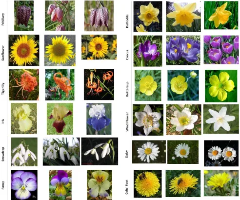
The Oxford flower dataset [13] was used to perform all our experiments. This dataset has ground truth segmentation for all images. The same criteria used by Nilsback and Zis-serman [13] was used to form our segmentation dataset. Flower classes that are under-sampled in the original dataset are removed. Therefore, following this criteria, five classes (Dandelion (Taraxacum), Lily of the valley (Convallaria majalis), Cowslip (Primula veris), Tulip (Tulipa) and Bluebell (Hyacinthoides non-scripta)) have insufficient images and are removed. This leaves 12 flower classes with a total of 753 images. Figure1shows examples of images in the dataset used for our experiments.

(4)

[image:4.595.48.540.40.450.2]

Figure 1: Example of images from the Oxford flower dataset (12 flower classes) used in our experiments.

divided into 80/20 for training/validation. We normalise all images by scaling RGB values to the range 0 - 1, before passing them to the deep neural networks. The RGB image annotation where first converted into a class label. For example, an RGB value of [255, 255, 0] value belonging to class one is replaced with [1, 1, 1] and so on. Finally, we converted the class labels into a binary class matrix (one-hot encoding) before passing them to our networks.

4 Network Architectures

We modified and reduced the number of parameters in our baseline deep convolutional neural networks, which includes FCN-VGG16 [11], ResNet18, ResNet34 and ResNet50 [8]. To provide instances for discussion, we describe four "Lite" CNN models, which are similar in architecture to our base networks but with a reduction in the number of parameters and a deeper architecture to avoid possible over-fitting.

We used only 2D 1⇥1 and 3⇥3 convolutions. The 2D 3x3 convolutions were converted

(5)

before and after each 3⇥3 convolutions to avoid possible overfitting. We used the 1⇥1

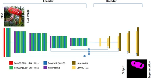
[image:5.595.56.550.110.366.2]

convolution filters because they can be seen as a linear transformation of the input channels, thus not increasing the network size further. Figure2shows our FCN-VGG16 "Lite" model.

Figure 2: Our "Lite" FCN encoder and decoder with blocks representing 2D Convolution (Conv2D), 2D Seperable Convolution (SeparableConv2D), Batch Normalisation (BN), Ac-tivation (ReLU) and upsampling layers.

The setup of ResNet50 "Lite" is slightly different. Since ResNet50 has a 1⇥1

convo-lution before and after each of its 3⇥3 convolutions, we converted only the 3⇥3

convo-lutions to separable convoconvo-lutions. Spatial pooling in the FCN "Lite" is carried out by four max-pooling layers, which follows some of the convolution layers. However, max-pooling is performed only once in the other networks (after the first convolution layer). In all the networks, we performed max-pooling over a 3⇥3 pixel window, with stride 2.

To further reduce parameters in our "Lite" CNN models, we introduced a simple global hyper-parameter (al pha = _{0.25,0.5,0.75,1.0_}) that allows trade-off between parameter-size and accuracy. This hyper-parameter allows the choice of right-parameter-sized model for appli-cation depending on problem constraints. Decreasing the value of alpha reduces the num-ber of parameters, whiles increasing this value, increases parameter size. The reduction of parameter-size is possible as our alpha is a multiplier of filter size in the networks and de-creasing filter-size usually shrinks network parameters. For example, after applying alpha = 0.25, 0.5 and 0.75 to a 2D convolution with 512 filters, the filter-size is reduced to 128, 256, 384 respectively. Note that at alpha = 1.0, the filter-size remains the same and the only tech-nique that reduces the number of parameters in our network is the 2D separable convolution used.

Table 1: Model parameters for the baseline and "Lite" models used in our experiments.

FCN’s Parameters ResNet18’s Parameters ResNet34’s Parameters ResNet50’s Parameters

(6)

All our architectures used the FCN-8 decoder style as described in [11]. We did not perform separable convolutions on these decoders as they already had a small number of parameters.

5 Experiments

For evaluation, we used the dataset detailed in section 3 to perform the following experi-ments:

• Pixel-wise segmentation into background and foreground (two classes) using the

base-line CNN models versus our "Lite" CNN.

• Pixel-wise segmentation of flowers into thirteen classes (including background) using

the original baseline CNN models versus our "Lite" versions.

• Evaluating results of global hyper-parameter (al pha=0.25,0.50,0.75,1.0) of "Lite" CNN models with the baselines.

5.1 Benchmarks and Setup

For benchmarking, we used the baseline CNN models on the Oxford flower dataset and compare the results to our "Lite" CNNs. In particular, we evaluated the number of parameters per model and the accuracy (pixel-accuracy and Mean IoU) per model.

For all models, we set the number of epochs to 200 and a batch-size of 6. We use categorical cross-entropy loss as the objective function for training the network and an Adam optimiser with an initial learning rate of 0.001. The learning rate was dropped by a factor of 0.1 whenever training plateaus for more than 10 epochs. Input images were resized to (224_⇥224).

There were huge variations in the number of pixels in each class as per the training samples. Therefore, we weighted the loss separately based on the actual class (know as class balancing). We applied median frequency balancing, which is the ratio of median class frequencies computed on the entire training samples divided by the class frequency. The implication of this is that larger classes in the training are given less weights whilst smaller ones are given more.

We trained all CNN models on a Linux server with three GeForce GTX TITAN X GPUs (12 GB memory each). The models were implemented using Python 3.5.3 and Keras 2.0.6 with Tensorflow backend and were tested on a Windows 10 computer with 64GB RAM and a 3.6GHz processor. The source codes for this project is publicly available here 1 _.

5.2 Metrics Used

We report two metrics from common pixel-wise segmentation evaluations that are variations on pixel accuracy and region intersection over union (IoU) [19].

• Mean Pixel accuracy: This tells us about the overall effectiveness of the classifier

and is defined in Equation1.

1

k

Â

i=1

nii

ti (1)

(7)

• Mean IoU: This compares the similarity and diversity of the complete sample set and

is defined in Equation2:

1

k

Â

i=1

nii

ti nii+Âk_j₌₁nji (2)

Where ti =Âki=1(Âkj=1ni j) is the total number of pixels of class i, ni j is the number of pixels of class i predicted as belonging to class j, nji is the number of pixels of class j predicted as belonging to classiandk is the total number of classes.

6 Results

[image:7.595.58.553.385.512.2]

Table 1 shows the number of parameters in our "Lite" model versus the baseline models. There is more than 60% parameter reduction with our "Lite-1.0" models and 77%, 90% and 97% with our "Lite-0.75", "Lite-0.50" and "Lite-0.25" models respectively when compared with baselines. This reduction in parameter-size suggests a decrease in computational com-plexity when training the "Lite" models.

Table 2: Pixel Accuracies and Mean IoU for both Baselines and "Lite" CNN models based on the Oxford Flower Dataset. We segmented flowers into two classes (flowers and back-ground). Best Results in Bold.

Baselines Lite-1.0 Lite-0.75 Lite-0.50 Lite-0.25 FCN-VGG16 Mean Pixel Accuracy (%)_{Mean IoU (%)} 97.23_93.58 97.11_93.32 96.88_92.81 96.52_91.99 96.30_91.56

ResNet18 Mean Pixel Accuracy (%)_{Mean IoU (%)} 95.75_90.31 95.66_90.15 95.57_89.98 95.64_90.07 95.09_89.00

Table 2 shows the results of all CNN models used to segment flowers from background (the two class problem). The baseline FCN-VGG16 and its "Lite" versions almost outper-formed all other CNN models. The model closest in performance to the FCN-VGG16 is FCN-ResNet50, which had 0.5% less mean pixel accuracy based on only the baseline mod-els. We then compare the accuracy of their "Lite" models with the baselines and realised just a tiny difference in mean pixel accuracy for the ResNet50 "Lite-1.0" and "Lite-0.75" (for ex-ample, only 0.02% and 0.08% respectively). The baseline FCN-VGG16 model also shows a similar difference in mean pixel accuracy with its "Lite-1.0" (only 0.12%). This comparison is also true when observing the mean IoU percentages, thus justifying the suitability of the "Lite" model for deployment on low-cost devices with limited resources.

Table 3 shows the results of the thirteen-class problem. Again, FCN-VGG16 outper-formed all the ResNet family of networks used in this experiment. There was only a 1.07% decrease in mean pixel accuracy when we compared the baseline ResNet50 with FCN-VGG16. Similarly, the baselines outperformed the "Lite" models by only a tiny margin, which reconfirms the suitability of the "Lite" models for deployments on low-cost and resource-limited devices, given their large parameter reduction.

(8)

[image:8.595.44.540.87.515.2]

Table 3: Pixel Accuracies and Mean IoU for both baseline and "Lite" CNN models based on the Oxford Flower Dataset. We segmented the flowers into thirteen classes (including background). Best Results in Bold.

Baselines Lite-1.0 Lite-0.75 Lite-0.50 Lite-0.25 FCN-VGG16 Mean Pixel Accuracy (%)_{Mean IoU (%)} 94.14_76.40 93.71_73.79 93.53_73.70 93.20_72.22 92.94_70.92

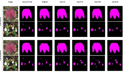
Figure 3: Multi-class segmentation: Sample test instances from the Oxford flower dataset with some segmentation errors.

"Lite" FCN-VGG16 models (especially "Lite-0.5" and "Lite-0.25"). However, considering the same instances, classification into two classes was not a problem for any of the classi-fiers. Figure 4 shows an example of segmented large and small flowers. Both the "Lite" and baseline CNN models were able to segment the larger flower well. Even though all the models’ performance were generally good, the baseline and "Lite-1.0" models segmented the smaller flowers better.

(9)

[image:9.595.59.549.38.323.2]

Figure 4: Two class (Background and Flower) segmentation: Sample test instances from the Oxford flower dataset with some segmentation errors.

to choose the appropriate "Lite" model for their application type.

Finally, our experiment revealed that even though our "Lite-1.0" models had near-comparable results with the baselines, reducing the value of alpha decreases the mean pixel accuracy and mean IoU by a rather small margin and increasing it increases mean pixel accuracy and mean IoU . Therefore using different alpha values gives the user the choice of appropriate parameter-size depending on the target deployment device and accuracy required.

7 Conclusion

We have introduced our "Lite" CNN models that reduce the number of parameters whilst making them deeper to avoid possible overfitting. Our experiments show the baseline FCN-VGG16 model to outperform all other baseline models by a small margin. Similarly, the baseline models outperformed the "Lite" versions, but this is expected considering the num-ber of parameter reduction in our "Lite" models. Typically, for the FCN which has 14.7 million parameters, this was reduced to 5.3 million and 0.3 million parameters for our "Lite-1.0" and "Lite-0.25" respectively. In most cases, the reduction in accuracy between baseline and "Lite" models is less than 0.5%, thus confirming the potential of the "Lite" models for deployment on low-cost and resource-limited devices. We have also shown that we can apply these CNN models to one of the most fundamental problems (that is segmentation) in plant phenotyping. We have also introduced a parameter (alpha), that can efficiently trade-off be-tween parameter-size and accuracy. This parameter gives the user the choice of appropriate parameter-size to match a target deployment device balanced against accuracy.

(10)

explore further parameter reduction and model matrix compression techniques to ensure the successful deployment of our models on these devices.

References

[1] Shubhra Aich and Ian Stavness. Leaf counting with deep convolutional and deconvo-lutional networks. arXiv preprint arXiv:1708.07570, 2017.

[2] Shubhra Aich, Imran Ahmed, Ilya Obsyannikov, Ian Stavness, Anique Josuttes, Keegan Strueby, Hema Sudhakar Duddu, Curtis Pozniak, and Steve Shirtliffe. Deepwheat: Estimating phenotypic traits from images of crops using deep learning. arXiv preprint arXiv:1710.00241, 2017.

[3] Nikos Alexandratos, Jelle Bruinsma, et al. World agriculture towards 2030/2050: the 2012 revision. Technical report, ESA Working paper FAO, Rome, 2012.

[4] Vijay Badrinarayanan, Alex Kendall, and Roberto Cipolla. Segnet: A deep convo-lutional encoder-decoder architecture for image segmentation. IEEE transactions on pattern analysis and machine intelligence, 39(12):2481–2495, 2017.

[5] François Chollet. Xception: Deep learning with depthwise separable convolutions.

arXiv preprint, pages 1610–2357, 2017.

[6] Emily L Denton, Wojciech Zaremba, Joan Bruna, Yann LeCun, and Rob Fergus. Ex-ploiting linear structure within convolutional networks for efficient evaluation. In Ad-vances in neural information processing systems, pages 1269–1277, 2014.

[7] Mario Valerio Giuffrida, Massimo Minervini, and Sotirios Tsaftaris. Learning to count leaves in rosette plants. In H. Scharr S. A. Tsaftaris and T. Pridmore, editors, Proceed-ings of the Computer Vision Problems in Plant Phenotyping (CVPPP), pages 1.1–1.13. BMVA Press, September 2015. ISBN 1-901725-55-3. doi: 10.5244/C.29.CVPPP.1.

URLhttps://dx.doi.org/10.5244/C.29.CVPPP.1.

[8] Kaiming He, Xiangyu Zhang, Shaoqing Ren, and Jian Sun. Deep residual learning for image recognition. InProceedings of the IEEE conference on computer vision and pattern recognition, pages 770–778, 2016.

[9] Forrest N Iandola, Song Han, Matthew W Moskewicz, Khalid Ashraf, William J Dally, and Kurt Keutzer. Squeezenet: Alexnet-level accuracy with 50x fewer parameters and< 0.5 mb model size. arXiv preprint arXiv:1602.07360, 2016.

[10] Jonghoon Jin, Aysegul Dundar, and Eugenio Culurciello. Flattened convolutional neu-ral networks for feedforward acceleration. arXiv preprint arXiv:1412.5474, 2014. [11] Jonathan Long, Evan Shelhamer, and Trevor Darrell. Fully convolutional networks for

semantic segmentation. InProceedings of the IEEE conference on computer vision and pattern recognition, pages 3431–3440, 2015.

(11)

[13] Maria-Elena Nilsback and Andrew Zisserman. Delving deeper into the whorl of flower segmentation. Image and Vision Computing, 28(6):1049–1062, 2010.

[14] Michael P Pound, Jonathan A Atkinson, Alexandra J Townsend, Michael H Wilson, Marcus Griffiths, Aaron S Jackson, Adrian Bulat, Georgios Tzimiropoulos, Darren M Wells, Erik H Murchie, et al. Deep machine learning provides state-of-the-art perfor-mance in image-based plant phenotyping. GigaScience, 2017.

[15] Michael P Pound, Jonathan A Atkinson, Darren M Wells, Tony P Pridmore, and An-drew P French. Deep learning for multi-task plant phenotyping. In Proceedings of the IEEE Conference on Computer Vision and Pattern Recognition, pages 2055–2063, 2017.

[16] Yifan Sun, Liang Zheng, Weijian Deng, and Shengjin Wang. Svdnet for pedestrian retrieval. arXiv preprint, 2017.

[17] Christian Szegedy, Wei Liu, Yangqing Jia, Pierre Sermanet, Scott Reed, Dragomir Anguelov, Dumitru Erhan, Vincent Vanhoucke, and Andrew Rabinovich. Going deeper with convolutions. InProceedings of the IEEE conference on computer vision and pat-tern recognition, pages 1–9, 2015.

[18] Christian Szegedy, Vincent Vanhoucke, Sergey Ioffe, Jon Shlens, and Zbigniew Wojna. Rethinking the inception architecture for computer vision. InProceedings of the IEEE Conference on Computer Vision and Pattern Recognition, pages 2818–2826, 2016. [19] Martin Thoma. A survey of semantic segmentation. arXiv preprint arXiv:1602.06541,

2016.

[20] Min Wang, Baoyuan Liu, and Hassan Foroosh. Factorized convolutional neural net-works. IEEE International Conference on Computer Vision Workshops, pages 545– 553, 2017.

[21] Jiaxiang Wu, Cong Leng, Yuhang Wang, Qinghao Hu, and Jian Cheng. Quantized con-volutional neural networks for mobile devices. InProceedings of the IEEE Conference on Computer Vision and Pattern Recognition, pages 4820–4828, 2016.

[22] Fisher Yu and Vladlen Koltun. Multi-scale context aggregation by dilated convolutions.

arXiv preprint arXiv:1511.07122, 2015.

[23] Xiangyu Zhang, Xinyu Zhou, Mengxiao Lin, and Jian Sun. Shufflenet: An ex-tremely efficient convolutional neural network for mobile devices. arXiv preprint arXiv:1707.01083, 2017.