Subdiffusion of nonlinear waves in two dimensional disordered lattices

EPL,98(2012) 60002 www.epljournal.org doi:10.1209/0295-5075/98/60002

Subdiffusion of nonlinear waves in two-dimensional disordered

lattices

T. V. Laptyeva, J. D. BodyfeltandS. Flach(a)

Max-Planck-Institut f¨ur Physik komplexer Systeme - N¨othnitzer Straße 38, D-01187 Dresden, Germany, EU

received 14 March 2012; accepted 25 May 2012 published online 27 June 2012

PACS 05.45.-a– Nonlinear dynamics and chaos PACS 05.60.Cd– Classical transport

PACS 63.20.Pw– Phonons in crystal lattices: Localized modes

Abstract – We perform high-precision computational experiments on nonlinear waves in two-dimensional disordered lattices with tunable nonlinearity. While linear wave packets are trapped due to Anderson localization, nonlinear wave packets spread subdiffusively. Various speculations on the growth of the second moment as tα

are tested. Using fine statistical averaging we find agreement with predictions from Flach S., Chem. Phys., 375 (2010) 548, which supports the concepts of strong and weak chaos for nonlinear wave propagation in disordered media. We extend our approach and find potentially long-lasting intermediate deviations due to a growing number of surface resonances of the wave packet.

Copyright cEPLA, 2012

Introduction. – Anderson localization (AL) —the halt of wave propagation in random potentials due to exponentially localized modes— was theoretically predicted over 50 years ago [1] and more recently observed within a variety of experiments, including optics [2–5] and matter waves [6,7]. These two fields are of keen interest, in that AL can be strongly altered by nonlinear Kerr effects in disordered photonic lattices [8–10], or atomic Bose-Einstein condensate interactions in optical lattices [11–15].

Research on wave dynamics in nonlinear disordered media largely focuses on wave packet evolution in one-dimensional (1-d) systems. Asymptotic subdiffusive spreading is observed. An extended debate of theories yielding different power exponents [16–22] appears to be clarified by the theoretical predictions and their numerical verifications in [23–27] for 1-d cases. Most studies focus on quartic nonlinearities which correspond to two-body interactions. Motivated greatly by experiment, e.g., in liquid-crystal optics [28,29] or at BEC-BCS crossovers in ultracold Fermi gases [30,31], one may also parametrize the nonlinearity exponent. This was done for the case of 1-d systems in [24,32]. The innovation here is to extend to two-dimensional (2-d) disordered systems. For such lattices that are multidimensional, disordered, and have

(a)_{E-mail:[email protected]}

variable nonlinearity exponents, spreading behaviors were broadly conjectured within [25]. The aim of this letter is to perform computational experiments to test the conjectures for asymptotic spreading in 2-d lattices with tunable nonlinearity. We also investigate the case of small nonlinearity exponents at which the theory predicts an anomaly in the number of wave packet surface resonances which should grow with ongoing spreading. We test the robustness of the theoretical predictions in this regime as well, where subdiffusion competes with fingering resonance instabilities.

Models. – The first model scrutinized is the general-ized disordered nonlinear Schr¨odinger equation (gDNLS), with the Hamiltonian

HD=

r

ǫr|ψr| 2

+2β|ψr| σ+2

σ+ 2 −

n

ψrψn∗

. (1)

equations of motion, derived from ˙ψr=∂HD/∂(iψ∗r) as

iψ˙r=ǫrψr+β|ψr| σ

ψr−

n

ψn. (2)

The above set of dynamic equations conserves the total energy HD, as well as the total norm S=_r|ψr|

2 . The 1-d version of the gDNLS has been extensively studied: for σ= 2 it relates to recent experimental photonics [10] and has been investigated numerically [23–27]. For a few integer values ofσ1-d simulations were presented in [32]. Simulations with non-integerσwere also performed [19] on short time scales without focus on asymptotic spreading.

The second model considered is the generalized 2-d Klein-Gordon (gKG) lattice with the Hamiltonian

HK=

r p2 r 2 + ˜

ǫru 2 r 2 +

|ur| σ+2

σ+ 2 + 1 4W

n

(un−ur) 2

,

(3) whereurandpr, respectively, are conjugated coordinates and momenta on the lattice siter, with an energy density

Er=

p2 r 2 +

˜

ǫru 2 r

2 +

|ur| σ+2

σ+ 2 + 1 4W

n

(un−ur) 2

. (4)

The positive numbers ˜ǫrhave uncorrelated random values drawn uniformly from an interval [1/2,3/2]. From ¨ur=

−∂HK/∂ur, the equations of motion read ¨

ur=−˜ǫrur− |ur| σ

ur+ 1

W

n

(un−ur). (5) This set of dynamic equations conserves only the total energy HK=_rEr. The 1-d version of the gKG has also been extensively studied, as it can be considered as a model for dynamics of anharmonic optical lattice vibrations in molecular crystals [33]. The quartic 1-d case was heavily used in numerical investigations [23–27], and different values ofσhave also been addressed [34].

Note, that in gKG the scalar value HK acts as the nonlinearity control. Several works [35–37] draw an approximate equivalence between the two models. For quartic (σ= 2) nonlinearity, this translates into

βS≈3WHK. It connects the KG initial parameters

HK and W to the total initial norm S and nonlinear parameter β of the corresponding quartic DNLS model. We generalize this condition to any powerσ

β

r

|ψr| σ

≈aσW

r

Erσ/2, aσ≡

8(σ+ 1)Γ(σ)

σ(σ+ 2)Γ2_(σ/2). (6) Neglecting nonlinear terms both eqs. (2), (5) reduce to an identical eigenvalue problem, giving a set of expo-nentially localized eigenstates (denoted as normal modes, NM) with frequencies λr in a spectrum of width ∆D= 8 +W in the case of gDNLS. Linear reduction for the gKG

1 2 3

σ -6 -4 -2 0 log 10 ε

6 8 10 12 14

W 1 2 3 log 10 V Self-Trapping Strong Chaos Weak Chaos

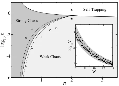
Fig. 1: Parameter space of the nonlinearity powerσ and the energy E _{of a single-site excitation. Dashed lines show the}

variation of the boundary obtained from variation of V (see inset). The symbols correspond to the set of parameters (σ,E₎

used in numerical simulations: “∗” for (2,0.3),(2,2.0); “+” for (0.5,0.00001),(0.7,0.0005),(1.0,0.006); “◦_{” for (1.3,0.025),}

(1.5,0.04); “×”for (0.5,0.005),(0.7,0.03). Inset: the depen-dence of localization volumeV on disorder strengthW. Squares (diamonds) are for the linear version of eq. (1) (eq.(3)). The gray region denotes an overall standard deviation. The solid line guides the eye.

is similar, but with squared frequenciesω2_r in a spectrum of width ∆K= ∆D/W= 1 + 8/W. We will focus mainly on analytics of the gDNLS, since it is straightforward to adapt results for the gKG using eqs. (6).

Expected regimes. – Consider the time-dependent normalized norm density distribution, zr≡ |ψr|

2

/S. The gKG counterpart is the normalized energy density distribution, zr≡ Er/HK. Distributions are analyzed by means of the second moment, m2=_r|r−m1|2zr, where the first moment m1 determines the distribution center. The second moment quantifies the squared width of the packet, hence, its spreading. The participation number,P= 1/

rz 2

Next we can estimate the average frequency spacing of NMs within the localization volume which is d= ∆D/V. The two linear frequency scales d and ∆D are expected to control the details of packet spreading. Nonlinearity introduces an additional frequency scale —the nonlinear frequency shift of a single oscillator, proportional to

βρσ/2 _{for the gDNLS, where ρ is the average norm} density of a packet. Note that the frequency shift is controlled by the nonlinearity and the density, and can therefore take different values relative to ∆D andd <∆D. Both the initial norm/energy density of a packet and its typical size were suggested [25] as the major control parameters for the dynamics at given W and σ. Under strong enough nonlinearity, a fraction of a wave packet (or even the whole packet) exhibits self-trapping [40]. For weaker nonlinearity (such that self-trapping is avoided), two possible dynamical outcomes are possible. The packet spreads in an intermediate regime of strong chaos with subsequent dynamical crossover into an asymptotic regime of weak chaos, or spreading starts directly in the weak-chaos regime. For single-site excitations the prediction turns into [25]

β(ρ/V)σ/2_{< d, weak chaos,}

β(ρ/V)σ/2> d, strong chaos, (7)

βρσ/2>∆D, self-trapping.

The spreading of nonlinear wave packets is due to an incoherent energy transfer between NMs inside the packet to nearby exterior NMs [23,25,41]. This incoher-ent transfer appears due to deterministic chaos which in turn is controlled by Chirikov-type nonlinear reso-nances [25]. The connection between the diffusion rate

D and the probability P(βρσ/2_)≈1−exp

−βρσ/2_d−1

for packet NMs to be in nonlinear resonance is conjec-tured as D∼β2_ρσ_(P(βρσ/2₎₎2_{. For large enough} nonlin-earities (i.e.,βρσ/2_d−1_{≫1) it followsP ≈1, hence nearly}

all modes interact in the regime of strong chaos. For weaker nonlinearities (i.e.,βρσ/2_d−1_{≪1) it turns to P ≈} βρσ/2_d−1_{,i.e., only a small fraction of modes resonantly}

interact in the regime of weak chaos. The subdiffusion is finally obtained fromm2∼ρ−1which leads to power laws

m2, P∼tα, α=

⎧

⎪ ⎪ ⎨

⎪ ⎪ ⎩

1

1 + 2σ, weak chaos,

1

1 +σ, strong chaos.

(8)

Note that forσ→0 both regimes yield normal diffusion. At the same time, the system dynamics should approach the behavior of the linear system (σ= 0) which is charac-terized by Anderson localization and therefore absence of diffusion. This is possible, since the prefactors in (8) will also depend onσ. As was shown in ref. [34], the prefactors indeed tend to zero in 1-d systems, leading to a vanishing of the corresponding diffusion constant.

Since the packet norm/energy density decreases in time during spreading, eventually the condition for strong chaos will be no longer satisfied —spreading will cross into the regime of weak chaos. Still, the duration of the strong-chaos regime can be greatly prolonged, so much that the crossover occurs at infeasible computation times.

In the regime of weak chaos, the number of resonances in the packet volume NRV and on its surface NRS are estimated [25] as

NRV∼βρσ/2−1, NRS∼βρ(σ−1)/2. (9) According to the above equation, for the 2-d case there are critical values of nonlinearity power: the number of volume resonances will grow for σ <2, likewise σ <1 for surface resonances. We therefore expect these critical values may manifest unusual effects in the course of packet spreading.

Numerical simulations. – The following numerics present only gKG results, for two reasons. First, the presence of a corrector scheme for gKG [24] allows two magnitude orders greater in integration. Second, all prior simulations of both models [23–27] show qualitatively similar results in a wide range of parameters.

To test the analytical prediction of eq. (8), we choose

W= 10, for which the localization volumeV ≈34. For an initial single-site excitation (L= 1) of energy E, regime boundaries from eq. (7) can be easily mapped into aE(σ) form using eq. (6). This gives a parameter space, shown in fig. 1.

We excite the central site by setting its momentum equal to √2E, while coordinates are equal to zero everywhere. The typical lattice size is 200×200 sites. Equations (5) are evolved using SABA-class symplectic integration schemes [42] with a time step of 10−1_{maintaining a relative energy}

conservation up to 10−2_{. For each set of parameters, we}

calculate the three measures m2, P, ζ. We then average over 400 disorder realizations. For each parameter set, we determine the spreading power-law exponent as local derivativeα(t)≡d log10m2/d log10t(see,e.g., [26]).

log

m

10

2

log t10

lo

gP10

2 4 6 8

log t10

l

m

log

z

10

r

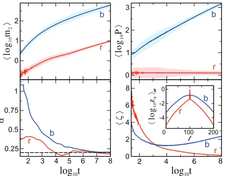
Fig. 2: (Color online) Numerics for “∗_{” in fig. 1. The parameters}

(σ,E) = (2,0.3),(2,2.0) correspond to the weak chaos ((b)lue) and self-trapping ((r)ed). Left column: average log of the second moment (top) and its power-law exponent (bottom)vs. log time. The dashed line is the theoretical expectation for the weak chaosα= 0.20. Right column: average log of participation number (top) and average compactness index (bottom)vs.log time. In both columns of the upper row the lighter clouds correspond to a standard deviation. Inset: normalized density distributions att= 108, averaged first over realization and then over them-index.

asymptotic compactness index is ζ≃2.36 (blue curve in fig. 2), meaning that the packet spreads, yet remains largely thermalized (ζ≈3). Large values of E satisfy the self-trapping regime. This behavior can be seen in the red curves of fig. 2 (E= 2.0, upper “∗” in fig. 1). A large portion of energy remains trapped on the initially excited site, while a much smaller portion subdiffuses. We thusly observe an increase of m2 (smaller portion subdiffusion), while P remains largely unaffected (large self-trapped portion). The compactness index approaches zero —a very good indication of self-trapping [26]. In the inset of fig. 2 we show normalized density distributions (averaged first over realizations, then over the m-index) for both regimes. The self-trapping regime reveals a characteristically trapped portion in the center.

Subdiffusion for 1< σ <2: weak chaos. Numeri-cal findings for “◦” in fig. 1 with parameters (σ,E) = (1.3,0.025),(1.5,0.04) are shown in fig. 3. Particularly in the lower left panel, the exponent α is shown to also asymptotically saturate. The two “I”-bars do not show error per se, rather their lower/upper bounds dictate the weak/strong-chaos expectations for α from eq. (8). The asymptotic saturations are approximately α≃0.3 for σ= 1.3 and α≃0.26 for σ= 1.5, which is quite close to their weak-chaos expectations of 0.278 and 0.250, respectively. The compactness values of ζ≃2.44,2.10 at

t= 107 _{remain fairly thermalized. Therefore, these two} points fully follow our expected theory of weak-chaos spreading.

1 1.5 2 2.5

〈

log

10

m2

〉

1.5 2 2.5 3

〈

log

10

P

〉

2 3 4 5 6 7 log ₁₀ t

0.25 0.5 0.75

α

2 3 4 5 6 7 log ₁₀ t

1 2

〈 ζ 〉

r r

r

r b

b

b

b

Fig. 3: (Color online) Numerics for “◦_{” in fig. 1. The}

parame-ters (σ,E) = (1.3,0.025),(1.5,0.04) are colored, respectively, as (r)ed and (b)lue. Left column: average log of second moment (top) and its power-law exponent (bottom)vs. log time. The I-bar bounds denote the theoretical expectations from eq. (8) for weak chaos (lower bound) and strong chaos (upper bound). Right column: average log of participation number (top) and average compactness index (bottom) vs. log time. In both columns of the upper row the lighter clouds correspond to a standard deviation.

Subdiffusion for σ1: strong chaos. Moving to the left in the parametric space (fig. 1), we cross the theoretical division between strong and weak chaos (two representa-tive points are shown by “×”). The corresponding numeri-cal results with parameters (σ,E) = (0.5,0.005),(0.7,0.03) are shown in fig. 4. Similarly, the I-bar bounds give weak-chaos (top) and strong-weak-chaos (bottom) expectations for the respective values ofσ. The asymptotic saturations for these two representative points are approximatelyα≃0.67 for σ= 0.5 and α≃0.57 for σ= 0.7, which is quite close to their respective strong-chaos expectations of 0.667 and 0.589. The compactness index fluctuates due to a slight asymptotic slope change in the participation numbers, nevertheless, it remains nearly thermalized (about 1.7 for

t= 106_{). Therefore, these two points follow our expected} theory of strong-chaos spreading.

1 2 3

〈

log

10

m 2

〉

1 2 3

〈

log

10

P

〉

2 3 4 5 6

log ₁₀ t

0.4 0.6 0.8 1

α

2 3 4 5 6

log ₁₀ t

2 3

〈 ζ 〉

r r

r r

b

b b

b

Fig. 4: (Color online) Numerics for “×_{” in fig. 1. The}

parame-ters (σ,E) = (0.5,0.005),(0.7,0.03) are colored, respectively, as (r)ed and (b)lue. Left column: average log of second moment (top) and its power-law exponent (bottom)vs.log time. The I-bars denote the theoretical expectations from eq. (8) for weak chaos (lower bound) and strong chaos (upper bound). Right column: average log of participation number (top) and aver-age compactness index (bottom)vs.log time. In both columns of the upper row, the lighter clouds correspond to a standard deviation.

hinted about σ= 1.0 for the 1-d KG model (cf. fig. 5 of [34]). Returning to our argument of resonance probabil-ity, this suggests both the weak/strong limits are invalid —the value ofP must be explicitly found. More than just a few modes contribute, but certainly not enough to yield strong-chaos regime.

Dimensional analysis. According to eq. (9), the concept of resonance probability may be viewed in the light of competition between surface growth vs. volume growth. Surface resonances more easily lead to the density leakage into modes exterior to the packet. This process in turn increases the packet’s perimeter, therefore yielding more surface resonances. Packets may thusly develop finger structures or fragment, perhaps leading to a fractal-like structure.

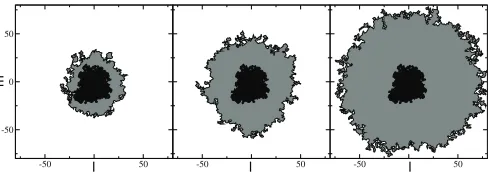
As a first hypothesis, we consider the normalized energy densities zr=Er/HK at t= 10

6_{, where an asymptotic} regime is reached (cf. figs. 2–5). In fig. 6, the largest contour path for zr10−

5 _{is shown, corresponding} roughly to the expanding packet’s surface. The left panel is for weak chaos with σ >1, the middle panel is for weak chaos with σ1, and the right panel is for strong chaos. Overlaid in black is the localized linear packet surface. A comparison of the coefficient α in figs. 3–5 can be observed. The wave packet in the left panel (α

corresponds to weak-chaos asymptotic) spreads less than that presented in the middle panel (α in between the weak- and strong-chaos limits), which spreads less than the right panel (αcorresponds to the strong-chaos limit). However, the boundary shape itself provides no further

2 2.5 3

〈

log

10

m 2

〉

2 2.5 3 3.5

〈

log

10

P

〉

4 5 6 7

log ₁₀ t

0.4 0.5 0.6

α

4 5 6 7

log ₁₀ t

1 2 3

〈 ζ 〉

r r

r r

g g

g

g

b b

b

b

Fig. 5: (Color online) Numerics for “+” in fig. 1. The parameters (σ,E) = (0.5,0.00001),(0.7,0.0005),(1.0,0.006) are colored, respectively, as (r)ed, (g)reen, and (b)lue. Left column: average log of second moment (top) and its power-law exponent (bottom)vs.log time. Similarly, I-bar bounds denote the theo-retical expectations from eq. (8) for weak chaos (lower bound) and strong chaos (upper bound). Right column: average log of participation number (top) and average compactness index (bottom)vs.log time. In both columns of the upper row, the lighter clouds correspond to a standard deviation.

m

l l l

Fig. 6: Largest contour forzr10−5att= 106. The black area

in the center is the contour for the linear case, while the panels, respectively, correspond to (from left to right): weak chaos with (σ,E) = (1.5,0.04), weak chaos with (σ,E) = (0.5,0.00001), and strong chaos (σ,E_{) = (0.5,0.005).}

Table 1: Box-counting dimension for the different regimes, zr10−

5_.

Regime (σ,E) Df

evidence: no boundary appears to be more fragmented or fingered than the others.

Therefore, we turn to a dimensional analysis of the contours. Binarizing zr at the threshold 10−

5_{, a} box-counting algorithm [44] is performed to extract the fractal dimension Df of the surface. The results were averaged over 100 different realizations and are presented in table 1. This further suggests: there are no clear and distinct fragmentation/fingering structures that might separate (in a geometric sense) the weak chaos atσ1 from the other two regimes.

Conclusion. – We have investigated the spreading of a single-site excitation under a variable power of nonlinearity within a 2-d disordered lattice, in particular for the Klein-Gordon case of eq. (3). For such a system, we numerically confirm the second-moment behavior of eq. (8), as first hypothesized in [25]. In particular, we verify the existence of both a weak-chaos and a strong-chaos regime. We distinguish these regimes by the number of resonant NMs in the wave packet that finally results in faster subdiffusion in the case of transient strong-chaos regime (nearly all modes become resonant), or, in slower subdiffusion in the case of asymptotic weak-chaos regime (the inter-mode resonances are rare), see eq. (8). In addition, an intermediate regime for σ1 is observed, with spreading behavior between the two limits of strong and weak chaos. We have performed an analysis of the wave packet geometries, but so far, strong fragmentation/fingering evidence in this regime, compared to the other regimes, is eluding. Possible future avenues along these lines may include lacunarity and density-density correlation measures. The behavior between the two regimes certainly remains open for future exploration, as well as pushing numerically the DNLS to achieve similar observations.

REFERENCES

[1] Anderson P. W.,Phys. Rev.,109(1958) 1492.

[2] Wiersma D. S., Bartolini P., Lagendijk A. and

Righini R.,Nature,390(1997) 671.

[3] Cao H.,Zhao Y., Ho S., Seelig E., Wang Q.et al., Phys. Rev. Lett.,82(1999) 2278.

[4] Chabanov A. A., Stoytchev M. andGenack A. Z.,

Nature,404(2000) 850.

[5] St¨orzer M., Gross P., Aegerter C.andMaret G., Phys. Rev. Lett.,96_{(2006) 063904.}

[6] Schulte T., Drenkelforth S., Kruse J., Ertmer W. andArlt J. J.et al.,Acta Phys. Pol. A,109_{(2006) 89.} [7] Roati G.,D’Errico C.,Fallani L.,Fattori M.,Fort

C.et al.,Nature,453_{(2008) 895.}

[8] Pertsch T., Peschel U.,Kobelke J., Schuster K., Bartelt H.et al.,Phys. Rev. Lett.,93(2004) 053901. [9] Schwartz T., Bartal G., Fishman S. andSegev M.,

Nature,446(2007) 52.

[10] Lahini Y., Avidan A., Pozzi F., Sorel M., Moran-dotti R. et al.,Phys. Rev. Lett.,100(2008) 013906. [11] Shapiro B.,Phys. Rev. Lett.,99_{(2007) 060602.}

[12] Skipetrov S., Minguzzi A., van Tiggelen B. and

Shapiro B.,Phys. Rev. Lett.,100(2008) 165301. [13] Billy J.,Josse V.,Zuo Z.,Bernard A.,Hambrecht

B.et al.,Nature,453_{(2008) 891.}

[14] Sanchez-Palencia L.andLewenstein M.,Nat. Phys., 6_{(2010) 87.}

[15] Modugno G.,Rep. Prog. Phys.,73(2010) 102401. [16] Shepelyansky D.,Phys. Rev. Lett.,70_{(1993) 1787.} [17] Molina M.,Phys. Rev. B,58(1998) 12547.

[18] Pikovsky A. and Shepelyansky D., Phys. Rev. Lett., 100(2008) 094101.

[19] Veksler H., Krivolapov Y. and Fishman S., Phys. Rev. E,80_{(2009) 037201.}

[20] Mulansky M.andPikovsky A.,EPL,90(2010) 10015. [21] Iomin A.,Phys. Rev. E,81_{(2010) 017601.}

[22] Basko D. M.,Ann. Phys. (N.Y.),326(2011) 1577. [23] Flach S., Krimer D. O. and Skokos C., Phys. Rev.

Lett.,102(2009) 024101.

[24] Skokos C., Krimer D. O., Komineas S.andFlach S., Phys. Rev. E,79_{(2009) 056211.}

[25] Flach S.,Chem. Phys.,375(2010) 548.

[26] Laptyeva T. V., Bodyfelt J. D., Krimer D. O.,

Skokos C.andFlach S.,EPL,91(2010) 30001.

[27] Bodyfelt J. D., Laptyeva T. V., Skokos C.,

Krimer D. O. and Flach S., Phys. Rev. E,84 (2011) 016205.

[28] Mihalache D., Bertolotti M. and Sibilia C.,Prog. Opt.,27(1989) 227.

[29] Christian J., McDonald G., Potton R. and

Chamorro-Posada P.,Phys. Rev. A,76(2007) 033834. [30] Bloch I., Dalibard J. and Zwerger W., Rev. Mod.

Phys.,80(2008) 885.

[31] Yan D., Kevrekidis P. G.and Frantzeskakis D. J., J. Phys. A: Math. Theor.,44(2011) 415202.

[32] Mulansky M.,Localization properties of nonlinear disor-dered lattices, Master Thesis, Diplomarbeit, Universit¨at Potsdam (2009).

[33] Ovchinnikov A. A., Erikhmann N. S. and Pronin

K. A., inVibrational-Rotational Excitations in Nonlinear Molecular Systems (Kluwer Academic/Plenum Publish-ers, New York) 2001.

[34] Skokos C. and Flach S., Phys. Rev. E, 82 (2010) 016208.

[35] Kivshar Y. S. and Peyrard M., Phys. Rev. A, 46 (1992) 3198.

[36] Johansson M. and Rasmussen K., Phys. Rev. E, 70 (2004) 066610.

[37] Johansson M.,Physica D,216(2006) 62.

[38] Schreiber M.and Ottomeier M.,J. Phys.: Condens. Matter,4(1992) 1959.

[39] Zharekeshev I. K., Batsch M. and Kramer B.,

Europhys. Lett.,34(1996) 587.

[40] Kopidakis G., Komineas S., Flach S.and Aubry S., Phys. Rev. Lett.,100_{(2008) 084103.}

[41] Krimer D. O. and Flach S.,Phys. Rev. E, 82(2010) 046221.

[42] Laskar J.andRobutel P.,Celest. Mech. Dyn. Astron., 80(2001) 39.

[43] Garc´ıa-Mata I.and Shepelyansky D., Phys. Rev. E, 79(2009) 026205.

MASSEY RESEARCH ONLINE

http://mro.massey.ac.nz/

Massey Documents by Type Journal Articles

Subdiffusion of nonlinear waves in

two-dimensional disordered lattices

Laptyeva, TV

2012-06-01