Automatic texture segmentation for content based image retrieval application

Abstract In this article, a brief review on texture segmentation is presented, before a novel automatic texture segmentation algorithm is developed. The algorithm is based on a modified discrete wavelet frames and the mean shift algorithm. The proposed technique is tested on a range of textured images including composite texture images, synthetic texture images, real scene images as well as our main source of images, the museum images of various kinds. An extension to the automatic texture segmentation, a texture identifier is also introduced for integration into a retrieval system, providing an excellent approach to content-based image retrieval using texture features.

Keywords Content-based image retrievalÆ Texture segmentationÆTexture identifierÆ Discrete wavelet framesÆMean-shift clustering

1 Introduction

Texture segmentation deals with the identification of regions where distinct textures exist, so that further analysis can be done on the respective texture regions alone. As far as this paper is concerned, there are three types of texture segmentation, which are the

super-vised segmentation, the unsupersuper-vised segmentation and the automatic segmentation. Supervised segmen-tation assumes prior knowledge of the types of textures which exist within the image. Unsupervised segmen-tation does not assume any prior knowledge of the types of textures, but it still needs to know how many textures there are in the image. Finally, automatic segmentation does not need any prior knowledge on either the type or the number of textures in the image. There are already a large number of supervised [1, 2] and unsupervised [3,4] texture segmentation algo-rithms in the literature. While the supervised and unsupervised techniques are very useful in a lot of applications, it is not very useful for our application of interest, since for both techniques the number of tex-tures present need to be given a priori. The particular application area with which this paper is concerned is content-based retrieval of art and museum artefact images, where the segmentation is to be performed on several thousand images. It is therefore inefficient to expect the number of textures to be manually provided for all the images. An automatic texture detection and segmentation algorithm is therefore needed to suit this kind of application.

In this paper, a novel automatic texture segmenta-tion, i.e. one without any a priori knowledge on either the type of textures or the number of textures in the image, is presented. The method uses a modified dis-crete wavelet frames (DWF) decomposition to extract important features from an image before a mean shift algorithm is used together with a fuzzyc-means (FCM) clustering to cluster or segment the image into differ-ent texture regions. The proposed algorithm has the advantage of high accuracy while maintaining low computational load. We will also show the advantage M. F. A. Fauzi (&)

Faculty of Engineering, Multimedia University, Jalan Multimedia, Cyberjaya, Selangor 63100, Malaysia e-mail: [email protected]

P. H. Lewis

School of Electronics and Computer Science,

University of Southampton, Southampton SO17 1BJ, UK e-mail: [email protected]

DOI 10.1007/s10044-006-0042-x

T H E O R E T I C A L A D V A N C E S

Automatic texture segmentation for content-based image

retrieval application

Mohammad Faizal Ahmad FauziÆPaul H. Lewis

Received: 7 January 2006 / Accepted: 19 March 2006 / Published online: 18 August 2006

of using the modified DWF over the standard DWF and the wavelet transform, and demonstrate how using the mean shift together with the FCM helps in speed-ing up the fuzzy clusterspeed-ing process.

This paper is organized as follows. Section2briefly reviews some of the texture segmentation algorithms available in the literature, before we explain the novel automatic texture segmentation algorithm in Sect.3. Section4 covers the experimental evaluation on sev-eral image data sets, including a real museum collec-tion. Section5describes how the proposed algorithm is extended to become a texture identifer, before it is evaluated in a content-based image retrieval (CBIR) system in Sect.6. This paper ends with a conclusion and potential future work on the proposed algorithm, presented in Sect.7.

2 Review of texture segmentation algorithms

Texture segmentation usually involves the combination of texture feature extraction techniques with a suitable segmentation algorithm. This section will briefly de-scribe some of the popular techniques used in texture feature extraction and texture segmentation algo-rithms.

2.1 Texture feature extraction

Among the feature extraction techniques used for texture segmentation are Gaussian Markov random field (GMRF), fractal dimension, Voronoi polygons, Gabor filters and wavelet decomposition. GMRF, fractal dimension and Voronoi polygons extract the textural characteristic by computing some parameters from the image. For example, in Manjunath and Chellappa’s paper [5], GMRF parameters are com-puted from non-overlapping regions of the image to be segmented. In the work by Chaudhuri and Sarkar [6], a box counting approach is used to estimate the fractal dimension of the original image, the high grey level image, the low grey level image, the horizontally smoothed image, the vertically smoothed image and the multi-fractal dimension of order two. Finally in Tuceryan and Jain’s work [3], the algorithm first builds the Voronoi tessellation of the tokens that make up the textured image, and a feature vector is computed for each Voronoi polygon.

Gabor filters and wavelet-based techniques on the other hand compute the textural characteristic by first transforming the image into the frequency domain and then dividing the domain into several frequency bands. The distribution of energy in each of these

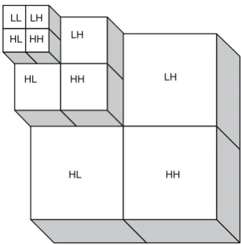
sub-bands is used as the basis for distinguishing different textures. The difference between the two techniques lies on the way the frequency domain is divided, as well as on the types of the filter used. In Paragios and Deriche’s work [1], the textured feature space is gen-erated by filtering the input and the preferable pattern image using Gabor filters. Wavelet-based techniques gain more and more attention in texture segmentation because of their multi-resolution property, which leads to multi-resolution segmentation. Multi-resolution segmentation is advantageous due to the extra infor-mation available through different resolutions, as it performs the segmentation algorithm over a range of spatial scales of the input image [7]. To illustrate multi-resolution segmentation, consider the pyramid-struc-tured wavelet transform (PWT) output image shown in Fig.1.

From the pyramid, it is clear that there are three different image resolutions forming the PWT output. Now the segmentation process can be applied from the top to the bottom of the pyramid. The four sub-images at the top of the pyramid are used as a four-dimen-sional data set to be segmented. The crude segmenta-tion results at this level are interpolated and passed to the next resolution. The segmentation at the next res-olution can then be performed by combining the data of that resolution with the temporary segmentation obtained from the previous resolution. The process continues and the final segmented image is obtained at the base of the pyramid. From this simple example only, it is clear that multi-resolution segmentation of-fers more advantages over single resolution techniques, where the lower levels of the pyramid help in refining the initial segmentation obtained at the top level.

LL

HH HL

LH

LH LH

HL HL

HH HH

In [8], Salari and Ling use the above multi-resolu-tion segmentamulti-resolu-tion algorithm using the PWT, while Chang and Kuo [9] experimented with the more com-plicated tree-structured wavelet transform. Besides wavelet, other techniques have also included multi-resolution property in the segmentation algorithm. In [10], Krishnamachari and Chellappa used the multi-resolution Gauss Markov random fields (GMRF) for texture segmentation. Coarser resolution sample fields are obtained by sub-sampling the sample field at fine resolution. The segmentation results from the coarser level are then propagated upwards to the finer reso-lution.

2.2 Texture segmentation

A texture segmentation algorithm can be developed by integrating the texture feature extraction techniques with a suitable segmentation method, such as the split-and-merge, region growing, estimation theory, clus-tering, relaxation and neural networks. The resulting texture segmentation, as previously mentioned, can be classified into three types, the supervised, the unsu-pervised and the automatic. Automatic texture seg-mentation, in particular, is a very challenging problem where correct identification of the number of textures inside an image is as important as the segmentation accuracy itself. Textured images, usually comes with a complicated data space, add to the challenges faced by researchers in this field. There are a very few automatic texture segmentation algorithms available in the liter-ature. With the exception of the work by Perry and Lowe [11], most automatic texture segmentation algorithms tend to first identify the number of textures within the image before an unsupervised clustering algorithm is carried out to segment the image into the desired number of segments. An example for this kind of segmentation can be found in the work by Porter and Canagarajah [12] and Liu and Zhou [13].

Back to the texture segmentation algorithms, Manjunath and Chellappa [5] opted for the nearest neighbour clustering method to merge the non-over-lapping regions of the image based on the GMRF parameters computed beforehand. Chaudhuri and Sarkar [6] use an unsupervisedk-means like clustering to the fractal dimension features computed to segment a scene into the desired number of classes. Tuceryan and Jain [3] use the feature computed from each Voronoi polygon in a probabilistic relaxation algo-rithm to identify the interior and the border regions of the textures, hence producing an unsupervised texture segmentation algorithm. Paragios and Deriche [1] produce a supervised texture segmentation algorithm

by minimizing a Geodesic active contour model objective function, where the boundary-based infor-mation is expressed via discontinuities on the statistical space associated with the multi-modal Gabor textured feature space generated during the feature extraction stage.

For the multi-resolution segmentation, Salari and Ling [8] use the pyramidal wavelet transform together with the k-means clustering. The four channels at the top of the pyramid are grouped into the desired num-ber of clusters by using the k-means clustering tech-nique. The resulting temporary segmentation is then labelled according to different clusters and normalized to avoid the domination of certain channels. The la-belled image is then interpolated and combined with the three channels at the next level. The process con-tinues until the labelled image corresponding to the base level is obtained. Another multi-resolution tex-ture segmentation technique using wavelet is proposed by Yang et al. [14] where they used the wavelet transform withkd-tree clustering.

On the other hand, Chang and Kuo [9] uses their tree-structured wavelet transform features with the fuzzy clustering. The image is first decomposed into tree-structured wavelet decomposition. Then, starting from the coarsest level, four leaf nodes corresponding to each tree nodes are clustered using the fuzzy c -means algorithm. The resulting output from the fuzzy clustering is a membership function. This membership function is then interpolated and combined with the leaf nodes or the membership functions available at the next level to provide features at that level. The process continues until the membership function correspond-ing to the root node is achieved. The segmented image can be obtained by assigning each pixel to the class in which it has the highest membership value. Krishn-amachari and Chellappa [10] used two techniques to estimate the GMRF parameters at coarser resolutions from the fine resolution parameters, one by minimizing the Kullback–Leibler distance and the other based on local conditional distribution invariance. The coarsest resolution data are first segmented by modelling a label field using MRF, and the segmentation results are propagated upwards to the finer resolution.

iterative stage. The growing ends when there exists no neighbouring element for which the distance of this element to the region is smaller than the threshold for the region. This algorithm however is computationally very intensive.

Porter and Canagarajah [12] use the standard wavelet transform together with k-means clustering and within cluster distance calculation to perform automatic texture segmentation. The wavelet trans-form is used to extract texture features, and the within cluster distance calculation is used to estimate the number of different textures within the image. Once the number of textures are known, thek-means clus-tering is applied to the data where k is the estimated number of texture regions. This method however is rather expensive computationally as it requires two completely different sets of algorithms, one to detect the number of textures present and another to segment them. Liu and Zhou [13] use wavelet transform to-gether with block-based segmentation to produce automatic texture segmentation. Similar to this paper, they also applied their segmentation algorithm for texture retrieval application. However, in the next section, we will show that the standard wavelet trans-form features do not provide a particularly good fea-ture space, hence will probably affect the segmentation result for different textures.

2.3 Comparison of texture segmentation techniques

There are also a few papers comparing the perfor-mance of several segmentation techniques. Du Buf et al. [15] compared seven different texture feature extraction methods which are the grey level co-occur-rence matrix, fractal, Michelle’s texture feature, Knutsson’s texture feature, Laws’ texture feature, Unser’s texture feature and curvilinear integration. Their paper is one of most important studies since they are the first to attempt to evaluate issues of image segmentation and boundary accuracy comparison in a quantitative framework. From the seven feature extraction methods tested, the Haralick, Laws and Unser methods gave the best overall results.

Chang et al. [16] experimented with three feature extraction methods and three segmentation algorithms. The three texture feature methods are the grey level co-occurrence matrix (GLCM), Laws’ texture feature and Gabor filtering techniques while the segmentation algorithms include the fuzzy clustering, square-error clustering and split-and-merge algorithms. The com-bination of Gabor filtering with the square error clus-tering was found to be the best among several

combinations. Gabor filtering more readily incorpo-rates multi-resolution information than the GLCM and Laws, therefore, resulting in much better segmenta-tion.

Pichler et al. [17] compared the pyramidal and tree-structured wavelet transform with the Gabor filtering in segmenting textured images. FCM clustering is used to obtain a segmentation based on computed texture features. The Gabor filtering was found to give the best segmentation result among the three techniques. Nevertheless, Gabor filtering was found to be very time consuming compared to the other two techniques.

3 A novel automatic texture segmentation algorithm Our proposed texture segmentation algorithm is based on multi-resolution clustering of texture data. Firstly, a feature extraction technique is applied to the image to obtain a series of texture coefficients at different res-olutions. Each coefficient represents pixels in the ori-ginal image. The coefficients are then clustered into an appropriate number of groups in the feature space, and each pixel is labelled to the group of its corresponding coefficients. There are several feature extraction tech-niques to be used in capturing texture coefficients. From our earlier work [18], we found that the DWF method [19] is the best texture algorithm in terms of the retrieval accuracy and computational speed, and thus have chosen to use it for the segmentation pur-pose as well.

Nevertheless, DWF results in quite a large number of coefficients, and this might slow the segmentation process. A modified DWF is proposed instead. Once the feature space has been constructed using the modified DWF, a suitable clustering algorithm can be used to cluster the data. However, since we would like to produce an automatic texture segmentation algo-rithm, the clustering algorithm needs to be able to identify how many clusters there are in the feature space. This can be done using the mean shift algorithm. The modified DWF, mean shift and the proposed segmentation algorithms are explained in the following section.

3.1 Modified discrete wavelet frames

wavelet transform isM2while the output of the DWF will have (3K+ 1)·M2 coefficients, where K is the number of decomposition levels. If we sample the DWF output every 2k samples, where k = 1,...,K is the level associated with a particular filtered image, the output will be exactly the same as the wavelet transform. The standard wavelet transform coefficients are actually a subset of a much larger set of DWF coefficients. It is therefore of more computational advantage to use the standard wavelet transform for segmentation instead of the DWF.

However, because of the sub-sampling, the wavelet transform coefficients are of very high variance, which could affect the clustering process quite badly. For example, the third level coefficients of the wavelet transform are sampled every eight coefficients both horizontally and vertically, and if we plot these into a feature space, there will not be well-defined clusters due to the high variance, even after applying some smoothing process. The DWF on the other hand does not suffer from this problem. While the wavelet transform is perfectly reconstructable, thus making it very good in some other fields, it is not very suitable for image segmentation, at least for the automatic case. One of the most important properties in achieving automatic segmentation is to be able to come up with a well-defined feature space; thus the wavelet transform is clearly unsuitable.

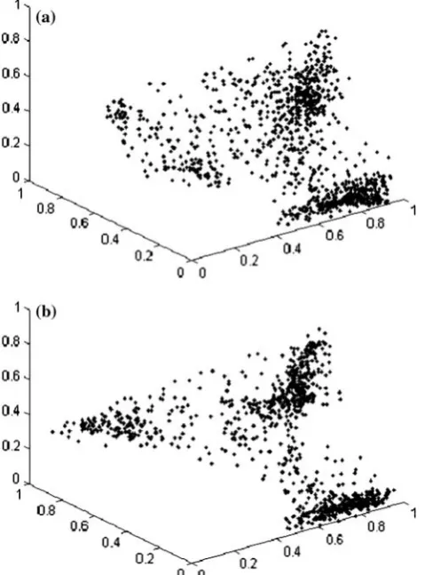
Nonetheless, it occurs that we can reduce the coef-ficients of the discrete wavelet transform to take the pyramid structure of the standard wavelet transform without significantly affecting the distribution of data in the feature space. If the coefficients of the DWF are carefully chosen rather than simply throwing away every other data point as in the wavelet transform, well-defined clusters can be preserved and the amount of data can also be reduced greatly. A simple yet reliable method is to take the mean of energy within distinct blocks. For each filtered image, the DWF coefficients are divided into distinct blocks of size 2k·2k, and the mean energy of the coefficients within the blocks are taken as the new coefficients of the DWF at that level. This results in data reduction of factor (2k·2k) for that particular filtered image. If this procedure is repeated for every filtered image of the DWF, we will have the same pyramid configuration as the wavelet transform but with better coefficients. Figure2 shows a 3D plot of coefficients at level 3 for both the wavelet transform and the modified DWF of the same image consisting of three textures. Notice that the data of the wavelet transform coefficients are poorly scattered and end up detecting four clusters instead of three.

3.2 Mean shift algorithm

Mean shift clustering is a relatively new clustering technique which finds possible cluster centres based on the density gradient of data, thus allowing unsuper-vised clustering to be performed. The rationale behind the density estimation based clustering approach is that the feature space can be regarded as the empirical probability density function (p.d.f) of the represented parameter. Dense regions in the feature space thus correspond to the local maximum of the p.d.f., that is, to the modes of the unknown density. Once the loca-tion of the mode is determined, the cluster associated with it can be delineated based on the local structure of the feature space.

Much of the work on mean shift clustering in image processing is done by Comaniciu and Meer [21–24], although the original idea was introduced by Fukunaga and Hostetler [25]. Due to its useful feature, mean shift has received considerable attention recently, especially in the field of image processing [26,27]. The idea of the mean shift is to shift all points in the feature space by a

Fig. 2 3D feature space plot a wavelet transform coefficient

significant amount until they converge to certain points. The convergence points are subsequently analysed to find possible cluster centres. A point is shifted to a new location based on the mean of all points within a radius h from the point itself. Theo-retically, the point will be shifted towards a local density maximum of the data set.

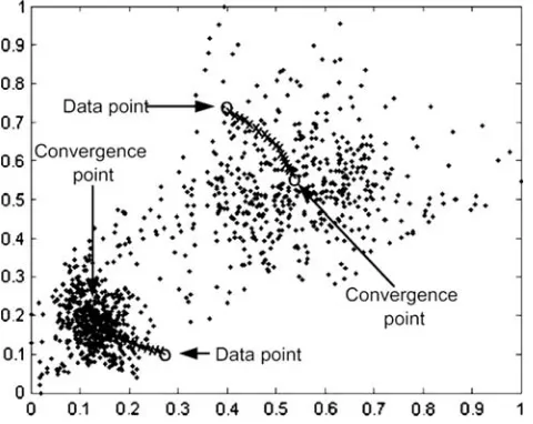
An example of mean shift convergence of a point is shown in Fig.3, for a two-dimensional case. From the same figure, the power of the mean shift-based clus-tering can be illustrated. The two clusters have arbi-trary shapes and the background is heavily cluttered with outliers. Traditional clustering methods would have difficulty producing satisfactory result. The two significant modes in the data space however will be clearly revealed in a kernel density estimation, making it possible for the mean shift procedure to detect both nodes. The associated basins of attraction then provide a good delineation of the individual clusters. In prac-tice, using only a subset of the data points suffices for an accurate delineation.

Comaniciu and Meer, however, used a simple near-est neighbour clustering to associate each data point with its cluster centre for their colour features. We find this approach is too basic to be used for texture fea-tures, since unlike colour, the distribution of texture feature data in the feature space is more complex and therefore needs a more robust clustering technique. Furthermore, since our method uses a multi-resolution feature extraction in DWF, the decision about cluster membership for a pixel only needs to be decided at the base level. The clustering output at all levels, except the base, only serves as intermediate results, and therefore is better represented by some sort of a membership function instead of a membership class. For these

rea-sons, we opt to use the FCM clustering to cluster the data, while the mean shift algorithm is just used to estimate the number of clusters and the cluster centres. The mean shift algorithm used in the proposed segmentation technique can be broken down into five processes:

– Data sampling. To reduce the computational load, a set of m points called the sample set is randomly selected from the data. Two constraints are imposed on the points retained in the sample set. The dis-tance between any two neighbours should not be smaller than h, the radius of the hypersphere Sh(x) and the sample points should not lie in sparsely populated regions. The latter condition is to avoid low density clusters. A region is sparsely populated whenever the number of points inside the sphere is below a thresholdT.

– Mode seeking. For each of the sample points, apply a mean shift procedure until the points converge to a stationary point. The mean shift computation for each sample points is based on the entire data set. The convergence points are considered as cluster centre candidates.

– Cluster centre derivation. Any subset of cluster cen-tre candidates which are sufficiently close to each other (for any given point in the subset, there is at least another point in the subset such that their dis-tance is less than h) defines a cluster centre. The cluster centre is the mean of the cluster centre can-didates in the subset.

– Cluster centre validation. Between any two cluster centres, a significant valley should occur in the underlying density. The existence of the valley is tested for each pair of cluster centres. If the density at any point between the two centres is below V·

(highest density between the two centres); 0 <V< 1, then a valley is observed and both centres are valid. If no valley was found, the cluster centre of lower density is removed from the set of cluster centres. – Clusters delineation. At this stage, each data point is

associated with a cluster centre using the FCM clustering technique.

We will discuss in detail all the parameters involved in the above algorithm in Sect.4.

3.3 Segmentation algorithm

Our proposed texture segmentation algorithm has a hierarchical structure and consists of two phases: a top-down decomposition phase followed by a bottom-up segmentation phase. Figure4 shows the flowchart of the algorithm.

3.3.1 Top-down decomposition phase

In the top-down decomposition phase, K-level DWF decomposition is performed. For a 2n·2nimage, this results in 3K+ 1 planes of 2n·2ndata. The amount of data is then reduced by applying steps described in Sect.3.1. This results in pyramid-structured coeffi-cients. At this point, we label the original image of size 2n·2nwith level index 0 (the base level), the four sub-images of size 2n–1 ·2n–1with level index 1 and so on. Since the DWF provide good spatial and frequency energy localization, we may take the energy value of

each modified DWF coefficient as an energy feature. However, the variance of the feature is still high since only one sample is used. By assuming that neighbour-ing DWF coefficients are identically and independently distributed, the variance can be reduced by performing a local averaging or smoothing operation.

On the one hand, it is desirable to have a large window to reduce the statistical variations. On the other hand, since a large window centred at points in the texture boundary region may contain multiple texture classes, the window size has to be small. To avoid this problem, we opt to use a sophisticated adaptive smoothing algorithm developed by Chang et al. [28], which repeatedly implements a simple local averaging operation until some criterion is satisfied. A typical smoothing operator is of the form

W¼ 1 16

1 2 1

2 4 2

1 2 1

0 @

1

A: ð1Þ

For an N· Nimage f(x, y), the iteration stopping criterion for a sub-image at thepth level is given by

Ck¼1:28 a 2pN

2_{; ð2Þ}

where

Ck¼ X

x X

y

Dk_fðx;yÞ

Wk1_fðx;yÞ

j j þ_jDk_{fðx;yÞj þ} ð3Þ

andais an estimate of the percentage of the number of boundary pixels (suggested value 1/N),is a very small number,Dk ” Wk– Wk–1, andWkmeans applying the smoothing operatork times.

The smoothed energy values are then normalized to the range between 0 and 1 within each node so that they can be conveniently used for segmentation in the bottom-up phase, as well as to make sure that no components will artificially dominate the clustering process.

3.3.2 Bottom-up segmentation phase

In the bottom-up phase, we start with level K and produce an intermediate segmentation result for level K– 1 using the four sub-images available at levelK. To generate the intermediate segmentation, the four sub-images of size 2n–K· 2n–Kare integrated in such a way that it can be viewed as four-dimensional 2n–K·2n–K data, before the mean shift algorithm is applied and provides us with the number of clusters detected in At each level, apply

feature smoothing to reduce variance

Integrate the 4 channels of the

coarsest level

Root level?

Yes Integrate the interpolated

membership function with the 3 channels of

the following level

Perform K-level DWF decomposition

followed by data reduction

Apply mean shift algorithm with fuzzy c-means clustering,

followed by interpolation

No

Assigned each pixel to the class in which it has the highest membership value

Top-down phase

Image, I(M,N)

Segmented Image, J(M,N)

Bottom-up phase

the data as well as the cluster centre positions. As mentioned in the last section, the FCM clustering is chosen above other clustering techniques and is applied to the four-dimensional data using the information provided by the mean shift. The FCM clustering algorithm is an iterative procedure described in the following:

Fuzzy c-means clustering algorithm Given M input data points {xm;m= 1,...,M}, the number of clustersC (2£C<M), and the fuzzy weighting exponent w, 1 <w<¥, initialize the fuzzy membership functions uc,m(0) withc= 1,...,Candm = 1,...,Mwhich are the entry of a C·M matrix U(0). Perform the following for iterationl= 1, 2,....

1. Calculate the fuzzy cluster centres vcl with vc=Pm=1M (uc,m)wxm/Pm=1M (uc,m)w.

2. Update U(l) with uc;m¼1=PCi¼1

dc;m

di;m

2

w1

; where ðdi;mÞ2¼ kxmvik2 and ||Æ|| is any inner product induced norm.

3. Compare U(l) with U(l+1) in a convenient matrix norm. If ||U(l+1)– U(l)||£e stop; otherwise return to step 1.

The value of the weighting exponent,w, determines the fuzziness of the clustering decision. A smaller value ofw, i.e.wis close to unity, will give the zero/one hard decision membership function, and a larger w corre-sponds to a fuzzier output. Our experimental results suggest thatw= 2 is a good choice. The advantage of using the mean shift algorithm together with the FCM clustering is demonstrated here. The FCM algorithm is not a fully unsupervised clustering method as it re-quires the number of clusters to be known a priori. Besides that, one other drawback of the FCM is finding the best way to initialize the fuzzy membership func-tion.

The FCM algorithm finds a local minimum of P

c=1 C P

m=1 M

uc,mw dc,m2 by solving uc,m and vc, and its output depends on the initial value of U(0). Various methods have been proposed on the best way to ini-tializeU(0)such as the maximin distance algorithm. But by using the mean shift, it provides the FCM with not only the number of clusters, but also the cluster cen-tres, meaning that the initial value of U(0) is already quite close to the final value ofU(0). Hence, part of the task of the FCM, which is to find appropriate cluster centres, is done. Experiments have shown that the FCM algorithm terminates after just a few iterations, thanks to the precise location of the cluster centres.

The output of the FCM is a 2n–K·2n–Kmembership function ofNc dimension, where Nc is the number of clusters. Each element of the membership function

describes the membership value with respect to a particular type of cluster and the sum of these elements is equal to 1. The membership function is then inter-polated to size 2n–K+1 ·2n–K+1 so that it has the same size with the data at the following level. For simplicity, a linear interpolation algorithm is used to interpolate the membership function.

At level K– 1, the interpolated membership func-tion is integrated with the three sub-images at this level resulting in an (Nc+ 3)-dimensional data set to be used for the next mean shift and FCM processes. These procedures of data integration, mean shift, clustering and interpolation are applied recursively from bottom to top so that we eventually obtain the segmentation result of the base level, i.e. the original image. The final crispy segmentation at level 0 can be determined by assigning each pixel to the class where it has the highest probability of membership. Note that the number of clusters detected by the mean shift algorithm can be different at each level. We might get a wrong number of clusters in the bottom level, but that is just an intermediate result, where not all data are utilized. What matter is the final segmentation result, after all data has been taken into account. The incorrect num-ber of clusters in the bottom level might be refined by the data at the higher levels.

Finally, the proposed texture segmentation algo-rithm works on the images of any resolution, and is not confined to dyadic length image only. For non-dyadic image length, the formula for the modified DWF re-mains the same except we introduce thefloorfunction when converting the coefficient to lower level. For example, an image with length 355 will have the length of 177 for level 0 coefficients, 88 for level 1 coefficients and 44 for level 2 coefficients. During the bottom-up segmentation process, the length will be converted back to the original length.

4 Experimental analysis

levels is found to be 0.2, while a suitable value ofTis one twentieth of the total data points at each level. The valley threshold, V, is set to 0.5. Figure5 shows the sequence of segmentation results obtained at each level for the composite texture image. In this example, the initial segmentation result obtained at level 2 al-ready gives a quite good segmentation and is used as a basis for higher level processing. It can be clearly seen that as the level increases, the segmentation result improves. This implies that the coefficients from the higher levels help in refining the boundary of the tex-tures, thus illustrating the advantage of multi-resolu-tion segmentamulti-resolu-tion.

We will now evaluate the performance of the algo-rithm for different numbers of textures within an im-age. The following section evaluates the performance on composite textures, synthetic textures, real scene images and museum images.

4.1 Composite texture images

In this section, the performance of the segmentation algorithm will be evaluated by its ability in identifying the correct number of textures in the image, as well as its precision in defining the boundaries of the seg-mented images. The precision is measured by com-puting the percentage of misclassified pixels in the

segmented images. We applied our texture segmenta-tion algorithm to several images of composite textures with size 256·256 pixels and 256 grey levels. Textures from the Brodatz album are used to make up the composite texture images by a cut-and-paste technique. Textures pasted are of either rectangular or square shape in order to make the computation of misclassified pixels easier. None of the textures used in our experiment can be discriminated by grey level values alone.

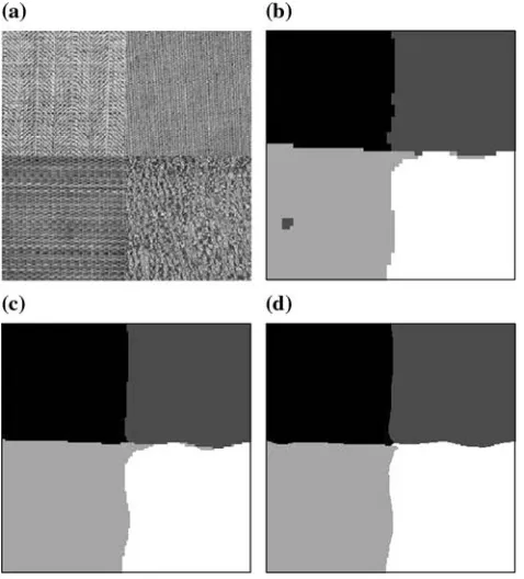
Figure 6 shows an example of applying the texture segmentation algorithm to a number of images with different numbers of textures. The two-textured image consists of texture D012 and D017, the three-textured image of texture D054, D074 and D102, the four-tex-tured image of texture D001, D011, D018 and D026, while the five-textured image consists of texture D001, D053, D065, D074 and D102. All the results in Fig.6 show a correctly identified number of texture as well as good segmentation. Altogether, we have applied our algorithm to 50 composite textures, and the results are summarized in Table1.

A return of 90% correctly detected the number of textures is very promising. Except for one of the three-textured images, which the algorithm detected to have five textures, all other incorrect results only miss by plus/minus one texture. Figure7shows an example of a wrongly detected number of textures. The image con-sists of texture D065, D066, D086 and D102. From the figure, it is clear that the incorrect segmentation is caused by the fact that the top half texture appears to contain two visually different regions. For the five incorrect cases, the cause is either the same problem as above, or the fact that two textures are almost the same visually.

Table 2 shows the percentage of segmentation er-rors for the five correctly segmented textures shown in Figs. 5and6. All the images give an error percentage of below 5% which is quite a low rate in texture seg-mentation. Notice that the more texture boundaries there are, the more difficult decisions must be made, resulting in an increasing number of misclassified pix-els. Non-boundary pixels seem to be well distinguished by the proposed algorithm. Altogether from the 45 correctly segmented images, we obtain an average of just 3.72% misclassified pixels.

Finally, we compare the performance of our algo-rithm with a segmentation technique based on the wavelet transform segmentation, i.e. the data to be clustered by the mean shift, and the FCM is generated by the standard wavelet transform instead of the modified DWF. Figure 8compares the performance of the modified DWF with the wavelet transform method

Fig. 5 Example of segmentation result a four-textured image

for the image in Fig.6d. Clearly, the wavelet transform fails to provide good clusters in the feature space resulting in a poor segmentation. Also, the sampling of poorly scattered data points during the mean shift results in a rather inconsistent segmentation for the wavelet transform-based segmentation. In this case, the modified DWF is therefore superior to the wavelet

transform in terms of segmentation performance, and is superior to the standard DWF in terms of compu-tational speed.

4.2 Synthetic texture images

Figure 9shows segmentation results for synthetic tex-tures composed of the + and L symbols. This texture pair has a spectrum with the same magnitude but dif-ferent phases. However, since it is difficult to pre-assign the classes for boundary pixels, it is difficult to compute the misclassified pixels. Thus, the evaluation for this particular problem is simply based on visual inspection. The algorithm successfully segments the two different textured regions. Since the illumination of both textures is the same, this example also shows that it is the surface texture, not the illumination con-dition that is being classified.

Fig. 6 Segmentation result for different numbers of textures

Table 1 Percentage of correctly detected number of textures No. of

textures in an image

No. images tested

Images with correctly detected no. of textures

No. of textures detected for the incorrect case

2 3 4 5

2 16 15 1

3 12 11 1

4 13 12 1

5 9 7 2

Total 50 45 (90%) 0 1 2 2

Fig. 7 Example of incorrect segmentation. The four-textured composite image is wrongly segmented into five segments

Table 2 Percentage of misclassified pixels Image Textures Misclassified

pixels

Percentage of error (%)

Figure5 4 1,654 2.52

Figure6a 2 621 0.90

Figure6b 3 1,771 2.70

Figure6c 4 1,615 2.46

4.3 Real scene images

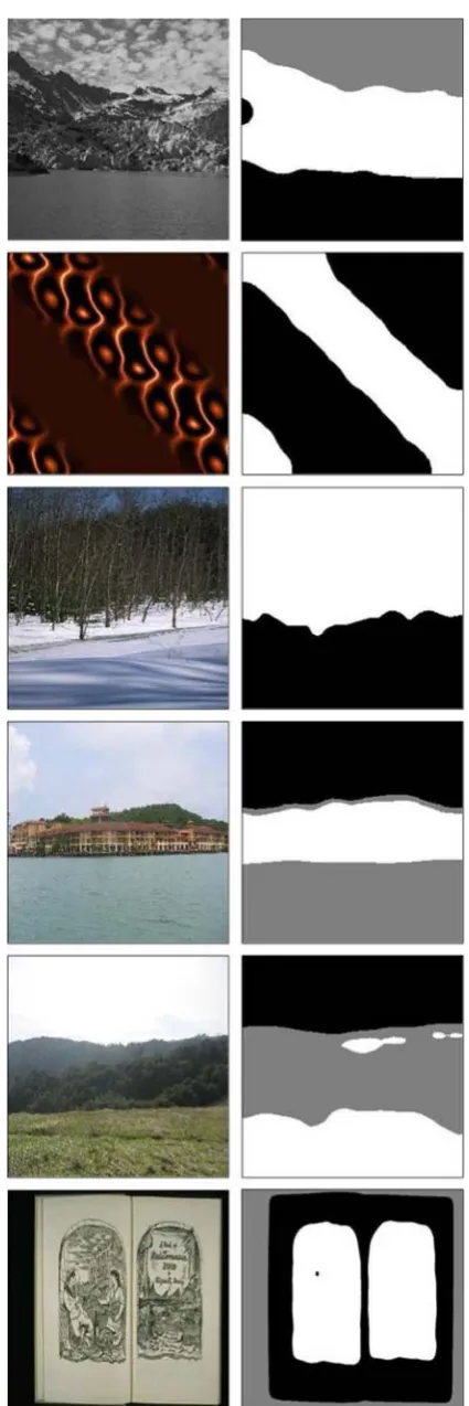
Figure10 shows the segmentation result on several real scene images as well as on a museum image. In the first, fourth and fifth images, the algorithm correctly identified the three regions and went on to segment the regions accurately. In the second and third images, the number of different texture segments in these images is two, and the algorithm again correctly identify and segment these images. As in the synthetic texture case, it is difficult to define an objective boundary for this example, thus the percentage of segmentation errors cannot be measured. However, from the few examples given, it is clear that the proposed algorithm works well in distinguishing real scene image textures.

The sixth image in the figure is an example of one of many various kinds of images in our museum collec-tions. In this example, the image is of an open book which consists of a textured region in the middle of the book and non-textured region in other parts of the book as well as a non-textured background. From the result of the segmentation, it can be seen that the algorithm manages to isolate the textured region of the book page from the non-textured regions. The result suggests that the proposed segmentation algorithm will be useful in our texture retrieval application.

4.4 Computational speed of the algorithm

The computational speed of the algorithm depends on two factors; the size of the image and how many seg-ments the algorithm perceives the image has. As men-tioned in detail in the previous section, there are several processes involved in the proposed algorithm, but the processes that are sensitive to the two factors above are the feature smoothing, the mean shift (data sampling, mode seeking, cluster centre validation) and the fuzzy clustering. For the first factor, the larger the image size, the higher the number of data points to be processed, in which the feature smoothing, data-sampling and the mode seeking processing time will all be longer.

The processing time for feature smoothing in partic-ular increases quite dramatically with the increase in image size. For the second factor, the higher the number of segments in an image, the higher the number of dif-ferent clusters in the data space, in which the cluster centre validation as well as the fuzzy clustering process will both take longer time to complete. The second factor however does not affect the computational speed as much as the first factor. Segmentation on a typical museum image of size 768· 768 with around three to five textured segments takes around 10 s on average. This will be very helpful in minimizing the time spent when creating a database of very large image collections.

4.5 The effect of segmentation parameters

Throughout the entire segmentation process, several parameters are encountered and these parameters may or may not have significant effect on the outcome of the segmentation result. These parameters include the radius,h, threshold,T, and valley,V, of the mean shift algorithm, the fuzzy weighting exponent, w, and the fuzzy stopping criterion,e, of the fuzzy clustering, and the estimate of the percentage of the number of boundary pixels, a, in the adaptive smoothing algo-rithm. In this section, we will discuss the significance of these parameters to the final segmentation result.

The mean shift algorithm is used to determine the number of texture regions in our segmentation algo-rithm; hence the three mean shift parameters affected only the final number of texture segments. The fuzzy clustering and adaptive smoothing parameters on the other hand contributed to the boundary accuracy of the segmentation of the known number of texture regions.

4.5.1 Mean shift parameters

The radius and threshold of the mean shift are very crucial in our segmentation algorithm. The radius

Fig. 8 Wavelet transform against DWF comparison. a Result using wavelet transform coefficients for the image in Fig.6d.

bResult using DWF coefficient

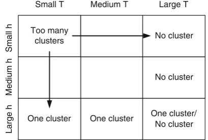
controls the number of segments or clusters in the image. It needs to be big enough so that the mean shift can converge on the correct cluster centres, but cannot be too big as it will result in all the points converging on the same cluster centre, i.e. only one big cluster is found. The threshold is used to make sure that the sample points do not belong to scarcely populated areas. This in turn contributes in controlling the size of the texture segments, i.e. in order for a particular texture to be considered as one texture region, the textured area should not be too small.

The radius and threshold are inter-related. When the radius is small, an appropriate threshold needs to be found so that it is proportional to the number of points in the circle of radiush. Figure11illustrates the effect of this inter-relation. A very large radius, depending on the threshold, will either detect only one big cluster or no cluster at all. Small radius with small threshold will produce too many clusters, thus increasing the probability of error. However, since we normalized the wavelet features to be between 0 and 1, the choice of radius and threshold can be determined quite easily by experiment. A radius of 0.2 is found to be suitable for our collection of museum images, while the value of the threshold, assuming that there will not be more than 20 clusters within the image, is taken as one twentieth of the total data points at each level.

The last mean shift parameter, the valley,V, is less crucial and is only used to check whether two cluster centres are actually in two different clusters. One hundred points are generated between the two cluster centres and the density of each point within the circle radius is calculated. If at any point the density is lower than V·(highest density of the two cluster centres), then it proves that the two cluster centres are in dif-ferent clusters. Otherwise, the two are considered to be in one cluster, and only one of the cluster centres will be considered as the final cluster centre. Therefore, the value of V does affect the number of clusters; the bigger V, the higher the number of clusters. It was found that a suitable value ofVis 0.5.

4.5.2 Fuzzy clustering and adaptive smoothing parameters

As mentioned before, the fuzzy weighting exponent, w (1 <w<¥), controls the fuzziness of the mem-bership function of the fuzzy clustering algorithm. The higher the weighting exponent, the more accurate the boundary accuracy of the segmentation. None-theless, bigger w also implies that there will be ‘‘holes’’ within the homogeneous texture segments. In

other words, while it may increase the boundary accuracy of the segments, the non-boundary region will not be as smooth. This problem can be solved by using higherwtogether with some relaxation process. However, as bigger w tend to make the membership function uniform, it does have an effect during the mean shift convergence of the following level. For this reason, the choice of w value should not be too big. From experiment, w= 2 was found to be the most suitable choice.

The fuzzy stopping criterion, e, does not have a major impact on the segmentation result since it only affects the location of the final cluster centres. The smaller the stopping criterion, the more iterations the fuzzy clustering will perform before settling the loca-tion of the cluster centres. However, there is very little difference on the cluster centre location that overall this parameter does not have a significant impact on the final outcome.

Finally, the estimate of the percentage of the number of boundary pixels, a, controls the shape of the clusters. The adaptive smoothing operation is applied to reduce the high variance of the wavelet coefficients, and the number of times the smoothing iteration is applied depends on a. Smaller a means applying the smoothing operation more times and may results in the data points being grouped together in one big cluster. Higher a, the extreme case means no smoothing operation at all, on the other hand may result in loosely populated clusters and might lead to too many clusters. The choice of a¼ 1

N as suggested by [28] is suitable for our application, whereNis the length of the image.

5 Texture identifier for CBIR

Content-based image retrieval becomes more and more important with the advance of the multimedia

and imaging technology. Historically, some of the popular CBIR systems have been the QBIC (Query By Image Content) [30] system developed by IBM, Virage [31] by Virage Inc., and Photobook [32] by MIT Media Lab. Colour, texture and shape are among the most commonly used retrieval features associated with CBIR, with texture feature being one of the most dif-ficult to solve. One of the reasons is that real images can have several different textures in a single image or they can also contain no texture at all. Good localiza-tion is therefore necessary to capture the local texture. As a solution, most CBIR systems opted for the more straight-forward block-based image decomposition, but while this approach can achieve quite a good locali-zation, it comes with quite a high computational load. The fact that the feature extraction process will always be applied for each and every block regardless of whether it is fully textured or not will have an effect on the retrieval performance as well, since more features mean more confusion for the algorithm. A segmenta-tion-based CBIR system can be used instead to avoid the problem.

In order to be used with a CBIR system, it is nec-essary for the segmentation algorithm not only to segment between textured regions, but also to distin-guish between textured regions and non-textured regions. Hence, only the feature vectors of the textured segments will be created and stored for matching purposes. Our proposed segmentation algorithm can discriminate not only between different textured regions but also between textured regions and non-textured regions, although it may or may not be able to segment different homogeneous or non-textured regions. For example, an image consisting of two textures on a dark background at the top and a bright background on the bottom will result in either three or four clusters using the proposed algorithm, two of them textured. The inability to segment non-textured region however is not important as we are only interested in the textured region. The non-textured region can be discarded using the algorithm to determine whether a particular segment is textured or not proposed by Porter and Canagarajah [12]. The basic idea behind their algorithm is to find the ratio of the mean energy in the low-frequency channels to the mean energy in the middle-frequency channels. Non-textured images (in which the grey level varies smoothly) are heavily dominated by the low-frequency channels in their wavelet transform. However, textured images have large energies in both the low and middle frequencies. For a three-level decomposition, the ratio can be computed between the mean energy in the four low-frequency channels (LL3,LH3,HL3,HH3) and the Too many

clusters

One cluster/ No cluster One cluster

One cluster

No cluster No cluster Small T Medium T Large T

Small h

Medium h

Large h

mean energy in the three middle-frequency channels (LH2,HL2,HH2) and is given as follows:

R¼LL3þLH3þHL3þHH3 LH2þHL2þHH2

: ð4Þ

If the ratio, R of a segment is above a certain threshold, then we can conclude that the particular segment is non-textured and thus no feature vectors should be created for it. Otherwise, if the ratio is below the threshold, then a feature vector is created for the segment.

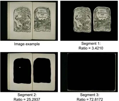
From visual inspection of the conducted experi-ments, a textured region usually gives a ratio of less then 10, while a non-textured region can be from 10 up to infinity. However, this is not always true as our collection of images is very large and it is impossible to visually inspect the ratio of all the textures. To avoid a situation where a genuine texture is missed, a threshold of 20 is used. It is less harmful for a non-textured being classified as textured than a textured being classified as non-textured as it will be completely ignored in cre-ating feature vectors. Figure12shows the same image example used in Sect.4.3, and the ratio of each of its segments. The textured segment clearly gives a small ratio to indicate its texturedness while the two non-textured regions have a much larger ratio.

The texture identifier hence is a useful tool in identifying significant texture regions within an image for feature extraction, while neglecting the non-tex-tured region of the image.

6 Integration with a retrieval system

We are now ready to integrate the proposed segmen-tation algorithm with a retrieval system. From the segmented regions, the last thing we need to do is to compute the feature vectors for the identified texture regions. We do not need to perform the wavelet decomposition again as we already have the original coefficients of the DWF when we perform the seg-mentation.

For this experiment, the following parameters are used. The number of decomposition levels is set to three levels and the wavelet basis is the Daubechies 8-tap wavelet. The mean subtraction can be applied by removing the local mean of the segmented region in theLLchannel to make it zero mean. The normalized Euclidean distance is used as the distance metric, while the standard deviation of energy and the number of zero crossings of all channels are used as texture fea-tures. For the identified texture regions, the features

are computed from the original DWF coefficients (not the modified ones used for segmentation) within the segmented texture regions only. This will create a feature vector that closely resembles the texture in that particular region. Finally, the luminence function is used to convert colour images to monochrome images. These parameters are so chosen because this experi-ment is part of our bigger project, which is to compare the segmentation-based approach with the block-based approach to texture retrieval, and we would like to use the same parameters for both approaches in order to produce a fair conclusion.

One might argue that we can simply take the cluster centres in each level and combine them to provide the feature vector. However, this is not true since the number of clusters found in each level might not be the same. Hence, it is difficult to compute the feature vector this way. Moreover, the cluster centre is based on the modified DWF, and not from the true DWF coefficients, thus might not be as good as the original DWF coefficients when used in texture matching be-tween several thousands texture images. Therefore, the proposed feature computation above will be used instead, as it is much easier to perform, and the dis-crimination performance of the original DWF coeffi-cients has been proved in our previous work [18].

A simple retrieval experiment is carried in order to observe the validity of this retrieval approach as well as its performance. Since this simple experiment is only intended to investigate whether the proposed algo-rithm can be successfully integrated into an image retrieval system, we used texture patches as the query to the system. A much better query selection scheme

where a user can load an image and then provide the query texture by choosing a specific region inside the image using a mouse can always be incorporated into the final system later. The retrieval experiment is tes-ted on a museum database of size 1,106. The retrieval performance was observed visually since we do not know how many similar textures there might be in the database. Nonetheless, as long as the top matches are visually similar to the query, it can be considered suc-cessful. Figure13 shows three examples of the seg-mentation-based retrieval. The line circling part of the image indicates the segmented region found by the algorithm to be similar to the query.

As can be seen, the retrieval system manages to retrieve visually similar textures to the query, and thus is very useful in texture retrieval of museum

collec-tions. However, one disadvantage of using segmenta-tion-based retrieval can be seen in the third example. Here the query image is a small stripe from one of the images in the database, and can be considered as a subset of a coarser texture. However, since the seg-mentation algorithm segments the coarser texture, the retrieved images does not actually correspond to the finer texture of the image; instead it corresponds to the coarser texture. In this example, the features of the finer scale and the coarser scale textures may be close (because the majority of the image consists of stripes); hence it still manages to retrieve all images consisting of stripes.

Nonetheless, apart from the lack of multi-scale property, the segmentation-based approach proves to be very good for CBIR application.

Fig. 13 Example of retrieval results of real museum collections. For each case, the query image is located at the top left, followed by the top 10 retrieved images (leftto

7 Conclusion and future works

In this paper, a new framework for automatic texture segmentation based on modified DWF and the mean shift algorithm is developed. By modifying the DWF, much better clustering is obtained on a reduced set of data, making possible the use of the mean shift algo-rithm to detect the correct number of clusters, and substantially reduces the processing time. The mean shift also provides the position of the cluster centres which effectively solves the problem of initializing the membership function in the FCM algorithm, and hence reducing the fuzzy iterations.

From the results of the experiments we can see that the proposed method can detect the correct number of clusters as well as segmenting the image correctly in composite textures, synthetic textures, real scene images and museum images, while main-taining the low computational load. The texture segmentation was then extended to be a texture identifier in order to use it in the image retrieval system. This is done by computing the ratio of en-ergy in the low-frequency channels to the enen-ergy in the middle-frequency channels, and observing whe-ther the ratio is below a certain threshold. The fea-ture vector of the identified texfea-ture region is then computed for matching purposes. From experimental result, the proposed segmentation-based retrieval system performs well in retrieving similar texture from a museum image collections.

Acknowledgments The authors are grateful to the Faculty of Engineering, Multimedia University, Malaysia and the School of Electronics and Computer Science at the University of South-ampton, UK for financial support. We are also grateful to the EU for their support under grant number IST_1999_11978 (The Artiste Project), and to our collaborators, the Victoria and Albert Museum, the National Gallery and the Research and Restoration Centre for the Museum of France for use of their images.

References

1. Paragios N, Deriche R (1999) Geodasic active contours for supervised texture segmentation. IEEE Comput Soc Conf Comput Vis Pattern Recognit 2:422–427

2. Talbar SN, Holambe RS, Sontakke TR (1998) Supervised texture classification using wavelet transform. In: Proceed-ings of the 4th international conference on signal processing, pp 1177–1180

3. Tuceryan M, Jain AK (1990) Texture segmentation using Voronoi polygon. IEEE Trans Pattern Anal Mach Intell 12(2):211–216

4. Jain AK, Farrokhnia F (1991) Unsupervised texture seg-mentation using Gabor filters. Pattern Recognit 24(12):1167– 1186

5. Manjunath BS, Chellappa R (1991) Unsupervised texture segmentation using Markov random fields models. IEEE Trans Pattern Anal Mach Intell 13(5):478–482

6. Chaudhuri BB, Sarkar N (1995) Texture segmentation using fractal dimension. IEEE Trans Pattern Anal Mach Intell 17(1):72–77

7. Ng I, Kittler J, Illingworth J (1993) Supervised segmentation using a multiresolution data representation. Signal Process 3(2):133–163

8. Salari E, Ling Z (1995) Texture segmentation using hierar-chical wavelet decomposition. In: Proceedings of the IEEE international symposium on industrial electronics, pp 216– 220

9. Chang T, Kuo C-CJ (1992) Texture segmentation with tree-structured wavelet transform. In: Proceedings of the IEEE-SP international symposium on time–frequency and time-scale analysis, pp 543–546

10. Krishnamachari S, Chellappa R (1997) Multiresolution Gauss–Markov random field models for texture segmenta-tion. IEEE Trans Image Process 6(2):251–267

11. Perry A, Lowe DG (1989) Segmentation of textured images. In: Proceedings of the IEEE computer society conference on computer vision and pattern recognition, pp 319–325

12. Porter R, Canagarajah N (1996) A robust automatic clus-tering scheme for image segmentation using wavelets. IEEE Trans Image Process 5(4):662–665

13. Liu Y, Zhou X (2004) Automatic texture segmentation for texture-based image retrieval. In: Proceedings of the international conference on multimedia modelling, pp 285– 290

14. Yang G, Hou Y, Huang C (2004) Texture segmentation algorithm based on wavelet transform and kd-tree clustering. In: Proceedings of the conference on robotics, automation and mechatronics, pp 987–990

15. Du Buf JMH, Kardan M, Spann M (1990) Texture feature performance for image segmentation. Pattern Recognit 23(3/4):291–309

16. Chang KI, Bowyer KW, Sivagurunath M (1999) Evalua-tion of texture segmentaEvalua-tion algorithms. In: IEEE confer-ence on computer vision and pattern recognition, pp 294– 299

17. Pichler O, Teuner A, Hosticka BJ (1996) A comparison of texture feature extraction using adaptive Gabor filtering, pyramidal and tree structured wavelet transform. Pattern Recognit 29(5):733–742

18. Fauzi MFA (2004) Content-based image retrieval of museum images, Ph.D. thesis, University of Southampton

19. Unser M (1995) Texture classification and segmentation using wavelet frames. IEEE Trans Image Process 4(11):1549–1560

20. Mallat SG (1989) A theory for multiresolution signal decomposition: the wavelet representation. IEEE Trans Pattern Anal Mach Intell 11(7):674–693

21. Comaniciu D, Meer P (2002) Mean shift: a robust approach toward feature space analysis. IEEE Trans Pattern Anal Mach Intell 24:603–619

22. Comaniciu D, Meer P (1999) Distribution free decomposi-tion of multivariate data. Pattern Anal Appl 2:22–30 23. Comaniciu D, Meer P (1999) Mean shift analysis and

applications. In: Proceedings of international conference on computer vision, pp 1197–1203

25. Fukunaga K, Hostetler LD (1975) The estimation of the gradient of a density function, with applications in pattern recognition. IEEE Trans Inf Theory IT-21(1):32–40 26. Jan T, Piccardi M (2004) Mean-shift background image

modelling. In: Proceedings of the international conference on image processing, pp 3399–3402

27. Lerdsudwichai C, Abdel-Mottaleb M (2003) Algorithm for multiple faces tracking. In: Proceedings of the international conference on multimedia and expo, pp 777–780

28. Chang T, Lin Y, Kuo C-CJ (1998) Techniques in texture analysis. In: Medical imaging systems techniques and appli-cations: computational techniques, Gordon and Breach Sci-ence Publishers, New York, pp 207–248

29. Brodatz P (1966) Textures: a photographic album for artists & designers. Dover Publications Inc., New York

30. Flickner M, Sawhney H, Niblack W (1995) Query by image and video content: the QBIC system. IEEE Comput 28(9):23–32

31. Bach JR, Fuller C, Gupta A (1996) Virage image search engine: an open framework for image management. In: Proceeding SPIE storage and retrieval for image and video databases, pp 76–87

32. Pentland A, Pickard RW, Sclaroff S (1996) Photobook: content-based manipulation of image databases. Int J Com-put Vis 18(3):233–254

Author Biographies

Mohammad Faizal Ahmad Fauzireceived the B.Eng. degree in electrical and electronic engineering from Imperial College, London, UK in 1999, and the Ph.D. degree in electronics and computer science from University of Southampton, Southamp-ton, UK in 2004. He is currently attached to the Multimedia University, Malaysia as a lecturer/researcher. His main research interests are in the area of biometrics as well as image, audio and video signal processing and analysis.