Agglomerative Forces and Cluster Shapes

Agglomerative Forces and Cluster Shapes

The Harvard community has made this

article openly available.

Please share

how

this access benefits you. Your story matters

Citation Kerr, William R., and Scott Duke Kominers. "Agglomerative

Forces and Cluster Shapes." Review of Economics and Statistics (forthcoming).

Published Version doi:10.1162/REST_a_00471

Citable link http://nrs.harvard.edu/urn-3:HUL.InstRepos:13244610

Terms of Use This article was downloaded from Harvard University’s DASH

Agglomerative Forces and Cluster Shapes

William R. Kerr

Harvard University and NBER

Scott Duke Kominers

University of Chicago

May 2013

Abstract

We model spatial clusters of similar …rms. Our model highlights how agglomerative forces lead to localized, individual connections among …rms, while interaction costs generate a de…ned distance over which attraction forces operate. Overlapping …rm interactions yield agglomeration clusters that are much larger than the underlying agglomerative forces themselves. Empirically, we demonstrate that our model’s assumptions are present in the structure of technology and labor ‡ows within Silicon Valley and its surrounding areas. Our model further identi…es how the lengths over which agglomerative forces operate in‡uence the shapes and sizes of industrial clusters; we con…rm these predictions using variations across patent technology clusters.

JEL Classi…cation: J2, J6, L1, L2, L6, O3, R1, R3.

Key Words: Agglomeration, Clusters, Networks, Industrial Organization, Silicon Valley, Entrepreneurship, Technology Flows, Patents.

1

Introduction

Agglomeration— industrial clustering— is a key feature of economic geography. A vast body of research now documents the prevalence of agglomeration in many industries and countries, and a number of studies have established its particular importance for …rm and worker productivity. Duranton and Puga (2004) and Rosenthal and Strange (2004) provide theoretical and empirical reviews, respectively. Moving from these measurements, researchers have recently sought to identify the economic rationales for …rm collocation and thereby the sources of the associated productivity gains. While the list of potential suspects dates back to Marshall (1920)— most notably labor market pooling, customer-supplier interactions, and knowledge ‡ows— we are just beginning to separate the relative importance of these forces.

Research on the spatial horizons over which di¤erent agglomerative forces act often takes one of two approaches. A …rst approach considers “regional”evidence. Examples include Rosenthal and Strange (2001, 2004), Duranton and Overman (2005, 2008), and Ellison et al. (2010). This approach begins by measuring the degree to which each industry is agglomerated across a chosen spatial horizon (e.g., counties, cities, states). A second step then correlates di¤erences in observed agglomeration to the traits of the industries. For example, we might observe that industries intensive in R&D e¤orts are more agglomerated when using counties or cities as a spatial unit than industries that do not depend upon R&D. Similarly, we might observe that industries with strong customer-supplier linkages are agglomerated at the regional level. A common inference from these patterns, as one example, is that knowledge ‡ows act over a shorter spatial distance than input-output interactions, as the knowledge-intensive industries are more heavily grouped together at the county level.

In parallel, a second strand of work considers “local”evidence on agglomerative interactions. Rather than discerning agglomerative forces from region-industry data, this line of research attempts to measure productivity gains directly at the establishment level. Prominent examples include Rosenthal and Strange (2003, 2008) and Arzaghi and Henderson (2008). A common approach is to estimate a plant-level production function that includes as explanatory variables the count of plants in the same industry observed within …ve miles of the focal plant, within ten miles, and so on (or within the same county, city, and state). These studies often conclude that spillover e¤ects decay sharply with distance, with the forces being orders of magnitude stronger over the …rst few city blocks than they are when …rms are 2-5 miles apart. These productivity studies are just the tip of the iceberg, however, with many related research strands measuring directly the distances over which humans or …rms interact (e.g., patent citations, commuting, etc.). As agglomerative forces depend upon these interactions, these studies also describe the local interactions that give rise to the clusters that we observe.

shapes and sizes of industries we observe in the data. The easiest way to observe this gap is to consider the spatial distances discussed by the two approaches. The regional literature often concludes that technology spillovers have a shorter spatial horizon than labor market pooling by comparing county- and city-level data. But counties have over 75,000 people in population on average, and the spatial size of counties is much greater than what “local”interactions suggest is the relevant range. If studies …nd that knowledge ‡ows decrease sharply within a single building (e.g., Olson and Olson 2003), why would we believe that we can infer useful comparisons of knowledge spillovers and labor pooling from regional data when the spatial scales of our data swamp the micro-interactions by orders of magnitude?

This project examines these issues theoretically and empirically. The core of our work is a location choice model that connects limited, localized agglomerative forces with the formation of spatial clusters of similar …rms. Agglomerative forces in our model are localized because …rms face interaction costs. Spillover bene…ts exceed these interaction costs at short distances, and thus …rms choose to interact. Beyond some distance, however, interaction becomes unpro…table and …rms no longer engage with each other. For example: while a …rm could learn useful technologies from another …rm 20 miles away, the costs of doing so may be too great to justify the e¤ort. Clusters are then the product of many small, overlapping regions of interaction. By building the cluster up from the micro-interactions, we obtain additional insights into the structure of clusters and the regional data we observe.

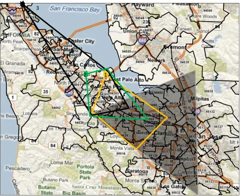
Silicon Valley is the world’s most famous cluster, and many observers credit its success to technology spillovers. Figure 1 illustrates the foundations of our theoretical framework using technology ‡ows in Silicon Valley. Downtown San Francisco and Oakland are to the north and o¤ of the map. The triangle in the bottom right corner of the map is the core of Silicon Valley. This core contains 76% of industrial patents …led from the San Francisco Bay area and 18 of the top 25 zip codes in terms of patenting.

To introduce our model, we describe the primary technology sourcing zones for three of the four largest zip codes for patenting in the San Francisco area that are outside of the core. Each focal zip code is marked with a star, and the other points of the shape are the three zip codes that …rms in the focal zip code cite most in their work. The orange zone (also labelled with a “1”) for Menlo Park extends deepest into the core. The green zone for Redwood City (“2”) shifts up and encompasses Menlo Park and Palo Alto but less of the core. The black zone for South San Francisco (“3”) further shifts out and brushes the core.

These technology zones are characterized by small, overlapping regions. None of the technol-ogy sourcing zones transverse the whole core, much less the whole cluster, and only the closest zip code (Menlo Park) even reaches far enough into the core to include the area of Silicon Valley where the greatest number of patents occur. While technology sourcing for individual …rms is localized, the resulting cluster extends over a larger expanse of land.1

over-Our model replicates these features and makes explicit that empirical observation of cluster size in the data does not indicate the length of the micro-interactions that produce the cluster. We show, however, that cluster shape and size does depend systematically on whether the localized interactions for …rms in an industry are longer or shorter in length. We demonstrate that a longer e¤ective spillover region, either due to weaker decay in bene…ts or lower interaction costs, yields a macro-structure with fewer, larger, and less-dense clusters. These regularities allow researchers to use cluster dimensions to rank-order spillover lengths even though micro-interactions are not observed. This connection helps bring together the diverse literature strands described earlier.

After deriving our theoretical predictions, we empirically illustrate the model using US patent data to describe di¤erences across technology clusters. Patent citations allow us to measure e¤ective spillover regions by technology. Di¤erences in these spillover regions relate to cluster shapes and sizes as predicted by the model. Technologies with very short distances over which …rms interact exhibit clusters that are smaller and denser than technologies that allow for longer distances. This empirical work primarily employs agglomeration metrics that are continuous, like in the metric of Duranton and Overman (2005), and we use traits of industries in the United Kingdom to con…rm the causal direction of these relationships (e.g., Ellison et al. 2010).

Our work makes several contributions to the literature on industrial agglomeration. Most importantly, we provide a theoretical connection between observable cluster shapes and the underlying agglomerative forces that cause them. Early “island” models of agglomeration— in which agglomerative forces act only within sites— implicitly feature maximal radius of interaction

0 (e.g., Krugman 1991, Fujita and Thisse 1996, Ellison and Glaeser 1997). More recently,

maximal radii also have been observed in more continuous models (e.g., Arzaghi and Henderson 2008, Duranton and Overman 2005). However, to our knowledge, our framework is the …rst to identify how variations in the maximal radius govern the shapes and sizes of clusters. At the core of this contribution is the simple mechanism of interaction costs among …rms. The resulting framework provides a theoretical foundation for inferring properties of agglomerative forces through observed spatial concentrations of industries. We identify settings in which such inference is appropriate, as well as key properties of agglomeration in such settings.2

Our central empirical contribution is a framework, motivated by our theoretical model, for meaningful analysis of agglomerative forces with continuous distance horizons. Previous work

lapping regions are also evident in the core itself and in other parts of the San Francisco region. These properties are also evident in labor commuting patterns in the region. Arzaghi and Henderson (2008) and Carlino et al. (2012) provide related visual displays.

2_{An additional contribution of our work, discussed in greater detail later, is to provide a micro-foundation} for using continuous spatial density measurements that center on bilateral distances between …rms. This class of metrics includes the popular Duranton and Overman (2005) metric.

considers how agglomerative forces a¤ect spatial concentration over di¤erent distance horizons, for example up to 75 or 250 miles (e.g., Rosenthal and Strange 2001, Ellison et al. 2010). Our framework is an important step towards jointly considering agglomeration at di¤erent distances (25, 75, and 250 miles) simultaneously. We hope that future research can similarly analyze other factors that govern clusters’shapes and sizes.

In addition to the related work already mentioned, our empirical work with patents relates to two other recent studies also considering continuous density measurements. Carlino et al. (2012) develop a multiscale core-cluster approach to measure the agglomeration of R&D laboratories across continuous space. In many respects, their metric’s nesting approach parallels our theo-retical focus on overlapping radii of interaction that build to a larger cluster. Likewise, some of their empirical results (e.g., clustering at local scales and at about 40 miles of distance) are also evident under our measures. Similarly, Murata et al. (2012) use continuous density estimations with patent citations to address the question of how localized are knowledge ‡ows. Their careful metric design allows them to bridge the well-known debate between Ja¤e et al. (1993, 2005) and Thompson and Fox-Kean (2005) and parse the underlying assumptions embedded in each study. Our work di¤ers from these studies in several ways, but the most important di¤erence is the theoretical focus and hypothesis testing about how di¤erent forms of interaction produce observable changes in cluster shapes and sizes.3

Section 2 presents our theoretical model. Section 3 describes our empirical strategy and data and provides initial evidence for our model’s building blocks using …rst- and later-generations of patent citations. Section 4 then undertakes speci…c measurements of technology-level spillover radii and tests our model’s predictions one at a time. Section 5 then introduces our continuous density measurements and tests the model predictions. The last section concludes.

2

Theoretical Framework

We now introduce a model of …rm location choice that generates large agglomeration clusters from smaller, overlapping spillover zones. To maintain consistency with previous work, we use the notation of Duranton and Overman (2005) whenever possible. We keep this initial exposition as simple as possible, and we conclude this section with a discussion of richer frameworks and extensions.

2.1

Basic Framework

There are N …rms indexed by i. These …rms i sequentially select their locations, denoted j(i),

from a …xed set Z _R2 _{of potential sites, each of which can hold at most one …rm.}4 _{Sites are}

drawn at random according to a uniform distribution in advance of any …rms’location decision

and are …xed. There are many more possible sites than …rms, i.e. _jZ_j N. To focus on

agglomeration economies, we assume that …rms compete in broad product markets. Location choice thus a¤ects the productivity of a …rm, but not its competitive environment.

The speci…c bene…ts of location j to a …rm are driven by intra-industry Marshallian forces

representing productivity spillovers that …rms generate by being in proximity to each other. Three common examples are customer-supplier interactions (e.g., reducing transportation costs for intermediate goods), labor pooling, and knowledge exchanges.

We denote by dj1;j2 the spatial distance between j1 2 R

2 _{and j}

2 2R2. We assume that the

deterministic bene…t of sitej ₂Z to a …rmi is given by

gj(i) X

i0₆=i

G(dj;j(i0₎);

for some continuous, decreasing functionG. The valuegj represents the degree to which spillovers

from other sites make sitej speci…cally attractive to …rms. We assume the standard comparative

static that G is decreasing, so that agglomerative forces decline over space. Additionally, for

simplicity, we assume that agglomerative forces act across all distances. That is, G(d) > 0 for

alld 0.

We assume that a …rm chooses randomly among sites j1; : : : ; j` over which that …rm would

be indi¤erent if forced to choose purely on the basis of spatial attraction.5 We also assume that …rms are not forward-looking, so that then-th …rm to enter,in(1 n N), chooses its location j =j(in)2Z to maximize gj(in) conditional upon the location choices of the …rst n 1 …rms.

2.2

Maximal Radius of Interaction

So far, our model has more or less followed a standard structure: proximity to resources and other …rms generates bene…ts, and these bene…ts decay continuously over distance. However, we now depart from this standard approach via a simple and natural additional assumption.

Assumption. A …rm must pay cost c to interact with another …rm.

These …xed costs c relate to the costs of transporting goods, people, or ideas across …rms.

Opportunity costs and search costs are the simplest examples, and these costs can be speci…c

to industries and spillover types. For example, accessing and understanding codi…ed technolo-gies likely requires a lower …xed cost of establishing interactions than that required for tacit technologies.6

Firms invest in establishing contacts when the bene…ts of doing so equal or exceed the

associated costs of interaction. Speci…cally, …rm i only invests in contact with a …rm i0 _if

G(dj(i);j(i0)) c. This de…nes a strict distance over which …rmi …nds interactions pro…table,

dj(i);j(i0) maxfd :G(d) cg:

Therefore, we immediately observe the following result.

Proposition 1. Firms at sites further than distance from a …rm i cannot pro…tably interact with i. That is, …rm i derives no direct bene…ts from the presence of …rms at locations j with

dj;j(i)> .

Proof: Immediate from text.

The key consequence of Proposition 1 is that agglomerative forces in practice act only over

…nite distances. We call the maximal radius of interaction (or just themaximal radius). The

maximal radius is (weakly) decreasing in the cost c and increasing in the levels of the decay

functionG. In other words, lower costs or weaker attenuation of bene…ts lead to larger maximal radii.

Our assumption that interaction costs are …xed is only to simplify the discussion below. One might naturally assume that interaction costs rise with distance; such an assumption would also generate the maximal radius described in Proposition 1. The ultimate technical condition required is that interaction costs exceed interaction bene…ts at some distance with a single crossing.

2.3

A Cluster-Based Theory of Agglomeration

We next examine how clusters form in our model and illustrate clusters’ properties. Figures 2a-2d provide a graphical presentation of the theory to build intuition. In these graphs, lightly colored circles are potential …rm locations, while …lled-in circles represent sites populated by …rms. Throughout this paper, we use these graphs to explain the model’s structure and depict the behavior of marginal entrants.

2.3.1 Basic De…nitions and Structure

We de…ne an agglomeration cluster to be a group of …rms located in sites interconnected by

bilateral interactions. Each …rm does not necessarily interact with every other …rm in its cluster,

but all …rms in a cluster are interconnected. Our measure of agglomeration counts the number of these clusters that are expected to arise; we say that …rms exhibit agglomeration if they typically occupy few distinct clusters. (The use of an expectation is necessary because …rms choose randomly when indi¤erent among sites.)

More formally: For j _{2 R}2_{, we denote by B}

d(j) fj0 2 R2 : dj;j0 dg the closed ball of

radius dabout j. For j ₂Z, we set

B0(j) B (j)_\Z:

This formula has a simple interpretation: _B0_{(j) is the set of potential …rm locations that can}

pro…tably interact withj under maximal radius .

In Figure 2a, we draw for each populated site a representative maximal radius within which

the bene…ts of interaction exceed the costs for …rms. For this example, _B0 _{for site B includes}

sites A and C. Sites A and C are the only locations within the maximal radius for Marshallian conditions .

We next expand our focus to consider sites that are outside of the pro…table spillover range of site j, but can be connected to j via a single interconnection. We de…ne _B1_{(j) to be the}

set of sites that can pro…tably interact with the sites in _B0_{(j) through one additional step. In}

Figure 2a,_B1_{(B)further includes the four additional sites within distance from site C that are}

outside of the spillover range of site B. We continue to iterate this process, successively adding additional sites that are more spatially distant to sitej but still connected to sitej by increasing numbers of interconnections (_B (j)for = 1;2; : : :). Formally, for any j ₂Z,

B (j) [

j0_2B 1_(j)

B0(j0):

Iterating this construction of clusters to its conclusion,_B (j)is the -cluster containingj ₂Z, de…ned by

B (j) 1

[

=0

B (j):

The -cluster containing sitej is the largest cluster of sites that 1) containsj and 2) is connected

by a chain of “hops” between sites j0 ₂ Z which can pro…tably interact. The complete set of

…lled locations in Figure 2a constitute the -cluster for site B in our example. The use of an in…nite index in the union de…ning _B (j) is ultimately unnecessary, as the …nitude of the set of sites implies that _B (j) =_B+1_{(j) = for some …nite .}

When the maximal radius is small, clusters are generally small. For two precise examples,

de…ne the lower and upper bounds on distances between sites as d minj16=j22Zdj1;j2 and

d maxj16=j22Zdj1;j2. When < d, B (j) = fjg for each j 2 Z. In other words, a maximal

containing a single …rm. By contrast, when > d, _B (j) = Z for all j ₂ Z. A maximal radius longer than the maximal distance between sites results in a single cluster for an industry.

If the maximal radius is and the …rst …rm locates at site j, and the cluster around j

contains available locations (i.e., _B (j)₆=_fj_g), then there is some site j0 _{2 B (j) which delivers}

positive deterministic utility ‡ows to the next entrant. It follows that if Marshallian forces are su¢ ciently strong, then …rms select sites in the cluster_B (j) until _B (j) is …lled. Iterating this analysis shows that when Marshallian forces are strong, …rms …ll clusters sequentially.

The sequential …lling of clusters explains how large-area clustering may arise in an industry even if agglomerative forces act only over short distances. Cluster sizes associated with a given maximal radius can be much larger than the underlying radius itself. Clusters may span large regions even if each …rm derives bene…ts only from its immediate neighbors.

A consequence of the maximal radius, however, is that clusters can reach their capacity, at which point the next entrant for the industry will locate elsewhere. In Figure 2a, the closest remaining site to the existing cluster is site X, but this location is beyond the spillover ranges of any of the populated sites in the cluster. As the marginal entrant cannot pro…tably interact with the cluster, it is indi¤erent among sites X, Y, Z, and any other unoccupied site. It will choose its location at random or based upon idiosyncratic preferences.

These observations suggest a natural notion of agglomeration. We say that …rms are(weakly)

more agglomerated with respect to maximal radius 1 than they are with respect to radius 2 if,

holdingN …xed, fewer clusters of …rms form when the maximal radius is ₁ than when it is ₂.

Formally:

De…nition 1. The level of agglomeration for maximal radius is _jZ_j , where is the

expected number of distinct -clusters _B (j) about sitesj ₂Z occupied by …rms.

Note that under this de…nition, agglomeration increases as the expected number of clusters decreases. Holding industry size constant, increased agglomeration therefore also corresponds

to increased cluster size. The additive term _jZ_j is a normalization that guarantees that the

level of agglomeration is always a positive number. We could equally well de…ne the level of

agglomeration for maximal radius to just be .

Our discussion of the marginal entry decision also highlights the core di¤erence between our structure and prior work. Without considering interaction costs, strictly positive spillover bene…ts exist at all distances due to the decay function G. Industries may di¤er in how fast or slow Marshallian bene…ts decay, but these di¤erences in Marshallian forces do not impact the number of clusters. Regardless of whether the potential spillover bene…t is large or miniscule, marginal entrants always select sites closest to the developing cluster regardless of distance (i.e., site X next in Figure 2a). As a consequence, each industry always forms a single cluster, and

entrants generically select sites in a …xed order. This is equivalent to the case in which _{! 1}

in our model. Once a …rst entrant picks a location, the set of sites …lled by the remainingN 1

Thus, the simplest framework does not provide a foundation for relating di¤erences in spatial concentration for industries to their underlying agglomerative forces. Yet, our intuitive addi-tion of interacaddi-tion costs provides addiaddi-tional tracaddi-tion by establishing a spatial range over which interactions are relevant. This localization in turn provides meaningful di¤erences in cluster formation. We now turn to these comparative statics.

2.3.2 Agglomeration due to Marshallian Advantages

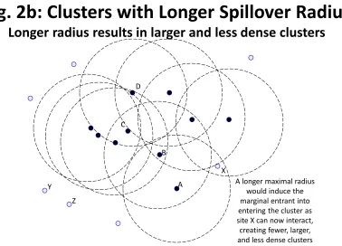
Figure 2b illustrates the consequences of a longer maximal radius for cluster formation. Under the larger maximal radius, the marginal entrant is no longer indi¤erent over sites, but would instead choose site X. Thus, a longer maximal radius is (weakly) associated with greater industry agglomeration as fewer clusters form in expectation.

More formally, recall that is the maximal radius for intra-industry spillovers, max_fd:

G(d) c_g: Since Z is …nite, small changes in do not a¤ect location choices. Larger increases in , either due to weaker attenuation in spillover bene…ts or lower interaction costs, can lead …rms to organize into fewer clusters. In fact, we may sign this change: …rms become (weakly)

more agglomerated when increases.

Proposition 2. A longer maximal radius of intra-industry spillovers leads to a (weak) increase in agglomeration.

Proof: See Appendix.

The idea behind the proof of Proposition 2 is intuitive. A …rm i that is indi¤erent across

sites chooses its location j(i) ₂ Z randomly. But until the sites in cluster _B (j(i)) are …lled, they are more attractive to …rms than are un…lled sites outside of _B (j(i)). If grows to ^, a

radius large enough to cause some cluster _B (j) to merge with another cluster (i.e. such that

B^(j) =B (j)[ B (j0) for some sitej0 2 B= (j)), then the expected number of clusters occupied

by …rms shrinks. Indeed, whenever a …rm locates in either _B (j) or_B (j0), subsequent …rms …ll all of_B^(j) before locating in or starting another cluster.

Three empirical implications of this analysis are evident in Figure 2b. First, industries with a longer maximal radius have larger clusters in the sense of having more …rms and covering a greater spatial area. Intuitively, a longer spillover radius makes sites at the edges of clusters attractive that are not attractive with a shorter radius. This induces marginal entrants into choosing these sites rather than starting new clusters. A longer radius can be due to weaker decay of spillover bene…ts or lower interaction costs.

if the radius is shorter. Thus, growth in cluster size is simultaneous with reduction in cluster density.

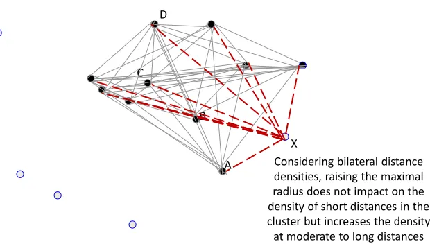
Our result that clusters due to a longer maximal radius are less dense is the same as saying that average bilateral distances among …rms within the clusters increase. The model’s structure, however, contains a much more powerful implication regarding spillover lengths and the complete distribution of bilateral distances within clusters. We draw out this implication in Section 2.3.4.

2.3.3 Ordering and Characterizing Agglomerative Forces

The theory suggests that longer maximal spillover radii are associated with fewer, larger, and less-dense clusters. It is feasible to use these observed traits in di¤erent industries to rank-order the radii associated with di¤erent spillovers. In empirical analyses below, for example, we provide suggestive evidence for the model by plotting an estimate of the maximal radii for di¤erent technologies against a measure of technology cluster density. This section introduces terminology and conditions required to jointly test these predictions using the continuous density estimation techniques employed in Section 5.

It is impossible to measure directly theGfunctions that determine the value of …rm clustering. However, observed spatial location patterns allow us to partially model the behavior of the

unobserved functionsG in a continuous manner.

Proposition 3. Holding …xed, and assuming that the G is di¤erentiable, an increase in _jG0_j

leads to a (weak) increase in the number of …rms clustered at small distances.

Proof: Immediate from text.

The decay of agglomerative forces across space correlates with observed distances between clustered …rms. Thus, we may understand the speed at which the bene…ts of localization decay by measuring the degree of localization at di¤erent distances. For an extreme example, if localization of …rms is constant across space, then we must have _jG0_j= 0. If localization gradients are very

sharp at short distances, then Proposition 3 implies that the underlying G function sharply

attenuates. Note that intercept valueG(0) isnot held …xed in Proposition 3. An implication of our framework is that, holding …xed, G(0) impacts the gradient _jG0_{j, but does not a¤ect the}

overall level of agglomeration.

Proposition 3 allows us to use the Duranton and Overman (2005) density estimations in Section 5 to characterize distributions continuously. Adding this more continuous structure to our model, we can compare the full distributions of industries to assess how longer maximal radii a¤ect the shapes of clusters. The predictions that clusters become larger and less dense become jointly visible. Moreover, we can observe this e¤ect’s in‡uence using regular step sizes in distance.

Let S denote the set of sites occupied by …rms in equilibrium, with many industries present

the maximal radius is , i.e. gj = 0— …rms locate randomly— when the maximal radius is .

We empirically proxy the set of potential sites Z with the observed set of actual sites S for

all businesses. With this assumption, density measures can quantify localization by comparing observed localization levels to counterfactuals representing the underlying distribution of eco-nomic activity typical for a bilateral distance. The null hypothesis is rejected if the localized density of …rms is a substantial departure from counterfactuals having (the same number of)

…rms occupying sites randomly sampled from S.7

2.3.4 Bilateral Distance Gradients in Agglomeration Clusters

There is an additional bene…t to connecting our model to these continuous structures. We earlier noted that our empirical implication of smaller, denser clusters for a shorter maximal radius is equivalent to saying that the mean bilateral density for clusters declines. The model, however, has a stronger implication for how spillover length in‡uences the distribution of bilateral distances within clusters.

Proposition 4. There is some > d so that whenever and 0 _{are such that d < <} 0 _{< ,}

then the mean intra-cluster …rm distance is (weakly) smaller when the maximal radius is than when it is 0_.

Proof: See Appendix.

This result describes a key comparative static across spillover lengths. When comparing two industries, we earlier established that the industry with the shorter maximal radius should exhibit denser clusters such that very close bilateral distances are common. This proposition further identi…es that this greater representation should be at its highest at the shortest bilateral distances possible (i.e., among locations very near to each other). This higher frequency should then (weakly) decline as one considers bilateral distances further from the shortest possible connections.8

To provide intuition, …rst consider the impact of the marginal entrant on the bilateral dis-tances in Figure 2c. As site X becomes part of the cluster, the set of bilateral disdis-tances grows to incorporate the bilateral distance from site X to every other populated site in the cluster into the spatial description. Some of the added bilateral distances are shorter than those that already existed in the cluster, with the distance between sites X and B, for example, being less than the distance between sites A and D. Yet, all of the additional bilateral distances are longer than the closest connections possible (e.g., those surrounding site C). Thus, as the cluster expands and becomes less dense, the relative impact on densities is most at the shortest possible connections and proceeds (weakly) outwards for some distance.

7_{As discussed in the empirical appendix of our NBER working paper and in the paper of Barlet et al. (2012),} this approach is slightly strained for the largest industries but is a reasonable baseline for most industries.

An empirical example can also help. Assume that the premium for proximity is higher for investment bankers than it is for accountants. We predict that clusters of investment bankers should exhibit shorter mean bilateral distances among …rms than clusters of accountants do. When comparing the spatial distributions of their clusters, Proposition 4 further indicates that the greater density for investment banking should be at its highest at the spatial level of being in the same building or on the same city block. When looking at …rms being …ve blocks away from each other, the spatial density for investment bankers can still exceed that of accountants, but the di¤erence should not be higher than it is when looking at being next door to each other. This requirement micro-founds use of continuous density metrics like that of Duranton and Overman (2005) in assessing whether di¤erences in agglomerative forces across industries yield meaningful deviations in agglomeration behavior. To summarize, we should empirically see that the greater density associated with a shorter maximal radius is at its maximum at the closest possible distance on the spatial scale and (weakly) declines thereafter for some distance. Even-tually, a distance is reached where the bilateral densities are the same even with the di¤erences in maximal radius. Continuing with our earlier example, the o¢ ces of investment bankers and accountants may be equally represented when looking at …rms that are ten city blocks apart.

After this point, a distance interval follows with relative under-representation for the cluster associated with the shorter maximal radius. Finally, once spatial distances are reached that rep-resent distances between agglomeration clusters for Marshallian industries, the relative densities again converge. In our example, accounting …rms should be more represented than investment bankers when looking at businesses 15-20 blocks from each other. This higher representation of accountants should then decline as we consider progressively longer distances that start to exceed the sizes of cities.

By contrast, our model generally does not make predictions for bilateral distances across Marshallian industries beyond the spatial horizons of individual clusters. The behavior of longer horizons depends upon the underlying distribution of cluster sites and it is thus ambiguous in our present framework. The median bilateral distance for all …rms within an industry, for example, can increase or decrease with a longer maximal radius depending upon the spatial distances among the multiple, growing clusters and the newly activated sites surrounding them.

2.4

Discussion

For simplicity, our base model only allows at most one …rm per site. Our results are unchanged if we allow multiple …rms to locate at each site, and assume that collocated …rms “congest”

each other. Speci…cally, we may extend our model by assuming that each site j ₂ Z has

a maximum capacity j 1, and that the set I(j) of …rms located at j must always have

jI(j)_j j. Congestion is modeled by assuming that …rmsi2I(j)6=;receive spillover bene…ts

of ^gj(i) (1=jI(j)j) gj(i): That is, spillovers to location j are divided equally among …rms

collocated at j. With these notations, our base model corresponds to the case that j = 1 for

all sitesj ₂Z. Even with congestion, the sequential location choice model is justi…ed: A …rm i

entering site j(i) has the potential to “crowd” its closest neighbors. But that …rm i can never crowd out another …rm i0 _{2 I(j(i)). Indeed, if …rm i}0 _{2 I(j(i)) were to exit j(i}0_{) = j(i) and}

relocate after the entrance of …rmi, then upon relocation,i0 would face the same location choice problem previously faced by …rm i. The ex ante optimality of j(i) for i would then show that

j(i) is the ex post optimal choice fori0.

Second, the micro-interactions across sites that are built into the model are readily gen-eralized. Our discussion and proofs focus on the simple case where spillover bene…ts do not transfer through the cluster. Interaction costs are incurred on a bilateral basis, and …rms at the periphery of a cluster only receive bene…ts from their immediate neighbors. More generally,

our predictions hold for any structure of bene…t transmission through the cluster so long as is

constant, as the spillover radius at the cluster’s edge is what determines the marginal entrant’s decision. We might also assume that with some probabilityp(d)<1…rms invest in contact with …rms of distance d away, with p declining in d (i.e. p0(d) <0). With our model’s structure, we can handle this case by simply replacing the function G(d) with G(d) p(d). Alternatively, if there is always some (possibly small) …xed probability that a …rm chooses its location randomly, as in the model of Ellison and Glaeser (1997), then our qualitative conclusions are maintained: an upwards shift in pleads to a fewer, larger, and less dense clusters.

Finally, the model does not include property prices. One way to introduce property prices to the model is to consider them as the consequence of wanting to be near a …xed feature (e.g., the city center). The version of the model in our NBER working paper shows that this extension does not materially a¤ect our predictions for Marshallian agglomeration so long as feature attraction e¤ects are not too strong.

3

Patent Technology Clusters

3.1

Overview of Empirical Strategy

over which knowledge interactions and technology ‡ows are occurring within clusters. In a generalization of the Silicon Valley case study in the paper’s introduction, we demonstrate how these knowledge ‡ows are limited in distance even within a single cluster. We also show how bilateral interactions form overlapping regions of interaction that cover a larger spatial area than the individual interactions of …rms do.

After establishing these properties generally, we use the patent data to calculate di¤erences in the lengths of maximal radii across technology groups. Some technology areas like semicon-ductors have very localized citation patterns where knowledge ‡ows decay rapidly with distance. Knowledge ‡ows in other technology areas operate e¤ectively over longer distances. After mea-suring these di¤erences across technologies, we turn to our basic model predictions that a longer radius of interaction generates larger and less-dense clusters (Propositions 1 and 2), showing that each of these basic predictions holds when considered independently. We do not investigate the number of clusters prediction as it is substantially more sensitive to empirical choices than the properties of clusters are.

Our …nal exercises present a uni…ed empirical framework for analyzing how technology cluster shapes and sizes di¤er across technologies in relation to their maximal radii of interaction. This framework brings to bear the joint nature of our three main predictions and the more subtle predictions of Propositions 3 and 4 with respect to rates of relative decay. These tests require that we depict the whole distribution of distances within a cluster and analyze the di¤erences in these shapes across technologies. We conduct these tests using a mixture of non-structured plots and the continuous spatial density metrics developed by Duranton and Overman (2005). These depictions provide greater insights into how observable cluster shapes provide information about the underlying agglomeration force.9

3.2

Patent Citations and Knowledge Flows

We employ individual records of patents granted by the United States Patent and Trademark O¢ ce (USPTO) from January 1975 to May 2009. Each patent record provides information about the invention (e.g., technology classi…cation, …rm or institution) and the inventors sub-mitting the application (e.g., name, address). Hall et al. (2001) provide extensive details about these data, and Griliches (1990) surveys the use of patents as economic indicators of technology advancement. The data are extensive, with over eight million inventors and four million granted patents during this period.

A long literature exploits patent citations to measure knowledge di¤usion or spillovers. A

number of studies examine the importance of local proximity for scienti…c exchanges, generally

…nding that spatial proximity is an important determinant of knowledge ‡ows.10 _{Additional work}

links these local exchanges and economic clusters. Carlino et al. (2007) …nd that higher urban employment density is correlated with greater patenting per capita within cities. Rosenthal and Strange (2003) and Ellison et al. (2010) …nd that intellectual spillovers are strongest at the very local levels of proximity. These empirical patterns closely link to ethnographic accounts of economic activity within clusters (e.g., Saxenian 1994).11

Patent citations thus o¤er us a unique opportunity to quantify di¤erences in spillover radii and cluster shapes. It is important, however, to recall several boundaries of this approach. First, patent citations can reasonably proxy for technology exchanges, but there are many other forms of knowledge spillovers that may behave di¤erently (e.g., Glaeser and Kahn 2001, Arzaghi and Henderson 2008). Second, several studies …nd that patent citations re‡ect Marshallian spillovers among …rms other than pure knowledge exchange. Breschi and Lissoni (2009) closely link citations to inventor mobility across neighboring …rms in their sample, and Porter (1990) emphasizes how technologies embodied in products and machinery can be transferred directly through customer-supplier exchanges. Our measurements below may encompass these e¤ects to the extent that they operate.

3.3

Patent Data Construction

Inventors are required to cite the prior work on which their current patent builds. The total count of citations made by USPTO domestic and foreign patents granted after 1975 is about 41 million citations. We …rst restrict this sample to citations where the citing and cited patents are both applied for after 1975. This restriction is necessary for collecting inventor addresses. Our second restriction is that both patents have inventors resident in the United States at the time of the invention with identi…able cities or zip codes. About 15 million citations remain after these restrictions. Our primary dataset further focuses on the 4.3 million citations that are made in a geographical radius of 250 miles or shorter from the citing patent.

To identify these distances, we extract zip codes from addresses given for inventors. This dataset combines both zip codes listed directly on patents and representative zip codes taken from city addresses where zip codes are not listed. Where multiple inventors exist for a patent, we take the most frequent zip code; ties are further broken using the order of inventors listed on the patent. The spatial radius is de…ned using geographic centroids of zip codes and the Haversine ‡at earth formula. We assign a distance of less than one mile to cases where the citing and cited patents are in the same zip code.

10_{See Ja¤e et al. (1993, 2000), Thompson and Fox-Kean (2005), Thompson (2006), and Lychagin et al. (2010).} Murata et al. (2012) measure the continuous density of patent citations.

Our analyses below consider how distances between zip codes in‡uence patent citation rates. Several issues with using inventor zip codes should be noted. A small concern is that our approach does not consider all of the zip codes associated with inventors for some patents, and this may lead to mismeasurement in our distance measure over short spatial scales (speci…cally, an upward bias on the minimum distance). As a check against this concern, we …nd very similar results when instead employing only patents with single inventors. More substantively, listed addresses can represent either home or work addresses. It would be nice to model both distances between work locations and distances between inventor home locations. Both of these distances can in‡uence technology di¤usion, and it is not clear which is more important. The patent data do not let us separate these two, however, and this measurement error biases us against …nding shorter spillover e¤ects.

To ensure that our results are not overly dependent upon this approach— especially with respect to the maximum radii that we calculate by technology— we also calculate a parallel set of distances using a match of USPTO patents to …rms in the Census Bureau (Balasubramanian and Sivadasan 2011, Akcigit and Kerr 2010). The Census Bureau data records identify the zip codes of each …rm’s establishments in a city. We thus take the patents identi…ed to be in Chicago for a particular …rm, for example, and assign them the zip codes of the …rm’s records.

Unreported analyses con…rm the spillover radii that we identify with our primary dataset.12

3.4

Knowledge Flows within Clusters

Our …rst analysis characterizes how knowledge ‡ows within technology clusters. To do so, we examine patent citation patterns, speci…cally di¤erences in spatial scope within clusters for …rst-generation citations compared to later …rst-generations of citations. This analysis is useful because it provides evidence for the interconnections among …rms built into our model’s structure. It also introduces the empirical framework that we use to calculate the maximal radius for each technology.

To introduce and clarify terminology, consider a sequence of patents where patent A cites patent B, patent B cites patent C, and patent C cites patent D. Using an arrow to indicate a

citation, our sequence is A_!B_!C_!D. Note that in this example the citations are moving from

patent A to patent D, while knowledge moves in the opposite direction. That is, patent A is building on patent B, and that is why patent A cites patent B.

We term a …rst-generation citation as a direct citation of prior work. In our example, these

would be A_!B, B_!C, and C_!D. When we discuss the distances over which …rst-generation citations occur, we are measuring the bilateral distances between these three pairs. We next de…ne a second-generation citation as the culmination of two steps in the citation chain: A_!!C

and B_!!D. When we discuss the distances over which second-generation citations occur, we are

measuring the bilateral distances between these end points, removing the intermediate step (i.e.,

A and C, B and D). Our simple example also has a single third-generation citation, A_!!!D,

and we would measure this distance as the bilateral distance between patents A and D.

Figure 2d continues with Figure 2a’s example to describe our empirical strategy. We place

into this graph the A_!B_!C_!D citation sequence just described. We contrived this example

to show a pattern where patent A would never have cited patent D directly according to our model. The distance from A to D is too great for the indicated maximal radius, but the distance can be bridged with the intermediate hops through patents B and C.

In reality, some measure of citations occur at distances that stretch across the full cluster (just as academics cite others at distances that span the globe). In fact, even if knowledge travels as in our model from patent D to patent A via sites B and C, we might still observe a patent A citing directly patent D (just as academics cite papers directly that they learned about through other papers). So, the model’s structure cannot be taken so strictly as to say that we should never observe citations at distances of the length between A and D. Nevertheless, we can learn a lot about relative distance of knowledge ‡ows by estimating the relative frequencies of citations by distance. Our model suggests that we should observe a higher frequency of …rst-generation citations when evaluating the shorter distances within clusters, as direct contact can occur at close proximities. Across longer spans, we should observe both fewer …rst-generation citations and more later-generation citations— indicative of knowledge transmission through a sequence of overlapping interactions.13

We demonstrate this pattern through some simple estimations illustrated in Figures 3a and 3b. For Figure 3a, we prepare a dataset that contains bilateral pairs of all zip codes that patent during the post-1975 period. To focus on local exchanges, we restrict these zip code pairs to those that are within 150 miles of each other. For each zip codez1, we then identify the number

of citations that it makes to the other paired zip code z2. To be conservative in our approach,

we do not examine interactions within the same zip code, and we exclude citations that …rms make internally among their inventions across zip codes.

With this dataset, we empirically model the count of citations that patents in zip code z1

make of patents in a second zip codez2 using the general form:

Citationsz1!z2 = exp

dz₁;z_2(Patents

z1 Patentsz2) ;

where as beforedz1;z2 denotes the distance fromz1 toz2. This expression suggests that citations

depend upon the interacted stock of patents in the two zip codes and upon the distance between the two zip codes, dz1;z2. We would anticipate < 0 if knowledge ‡ows are declining with

dis-tance, and >0if a greater number of patents in the two zip codes provides more opportunities for citations. Rearranging this expression gives

ln(Citationsz1!z2) = dz1;z2 + ln(Patentsz1 Patentsz2);

which is the starting point for our …rst estimating equation. We make three further modi…cations. First, beginning with the citations outcome variable, zero citations may be observed even where patents exist (and this lack of exchange is important information). Our base estimation thus takesln(1 +Citationsz1!z2) to be the citations outcome variable, and we model other variations

below to test the sensitivity of theln(X)_7!ln(1 +X) transformation.

Second, there are multiple ways that one might de…ne distance to potentially allow for non-linear e¤ects that our model emphasizes. Our …rst approach is to estimate distance’s role in a

non-parametric format using a series of indicator variables I( ) for distance bands between zip

codes. We de…ne a vector of distance bands as within one mile (but not the same zip code), (1,3] miles, (3,5] miles, (5,10] miles, (10,15] miles, . . . , (95,100] miles, and (100,150] miles. We denote

the set of distance rings as DR, and we include separate indicator variables for each distance

band up to zip codes being (95,100] miles apart. Our _dr coe¢ cients will thus measure the

di¤erence in citation rates observed for a distance interval compared to the reference category of being more than 100 miles apart in the technology cluster.

Finally, theln(Patentsz1 Patentsz2)control is important, but it is also weak. Our initial tests

With these three adjustments, our core estimating equation for Figure 3a becomes,

ln(1 +Citationsz1!z2) = +

X

dr2DR

dr I(dz1;z2 =dr) + ln(Patentsz1 Patentsz2)

+ ln(1 +Expected Citations_z1!z2) +"z1!z2: (1)

The solid line in Figure 3a plots the dr coe¢ cients for …rst-generation citations like the A!B

example discussed in Figure 2d. First-generation citations are quite concentrated at short dis-tances and decline almost monotonically with increasing distance. The citation premium loses half of its strength by (15,20] miles, and zip codes that are 40 miles or more apart are very similar to those in the reference category of being 100-150 miles apart. This substantial decay echoes very closely the localized networking results of Arzaghi and Henderson (2008) and the spillover estimations of Rosenthal and Strange (2003, 2008). It is important to recall that we have excluded interactions within the same zip code, in order to be conservative. The within-zip code citation premium is larger in magnitude than that observed for neighboring within-zip codes within one mile of each other.

The dashed line in Figure 3a graphs the spatial patterns of second and third generations of

patent citations, equivalent to the A_!!C and A_!!!D example. To construct the

second-generation citation pro…le for zip code z1, we start with the patents that were cited directly by

…rms in zip code z1 within a 250-mile radius around zip code z1. We then collect the citations

that those patents made to other patents within 250 miles of their zip code. We then calculate

the distances from the focal zip code z1 to these citations, and we will focus again on the

second-generation citations that fall within 150 miles of zip code z1. We take this approach to

provide very ‡exible local distances. Note, for example, that the distance from zip code z1 to

a given second-generation citation can be closer than the …rst-generation citation that links it. We repeat the same process for third-generation citations. The speci…cation (1) is again used to compare rates in local distances to the rates that exist over 100-150 miles.

…xed e¤ects remove persistent di¤erences that exist across zip codes in citation counts such that we are exploiting only variation in how much zip codez1 cites other zip codes in its technology

cluster more or less than typical for zip codez1. The second estimating equation takes the form

ln(1 +CitationsRing_z1!dr) = X

dr2DR

dr I(dz1;z2 =dr) + ln(Patents

Ring dr )

+ ln(1 +Expected CitationsRing_z1!dr) + _z1 +"z1!dr: (2)

These regressions measure the _dr coe¢ cients relative to the activity observed in excluded

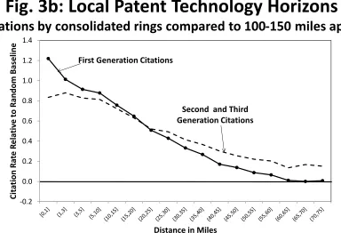
dis-tance ring of 100-150 miles apart. The solid and dashed lines in Figure 3b again plot the …rst-and later-generation citations, respectively. At very short distances, …rst-generation citations show greater relative frequency compared to later-generation citations. The di¤erences reverse at moderate distance ranges.

Appendix Tables 1, 2a, and 2b provide complete details on these estimations and descriptive statistics. Appendix Tables 2a and 2b report very similar results to Figures 3a and 3b, respec-tively, when zero-citation cells are excluded, when we drop the expected citations controls, and when we include own-zip code citations.

These di¤erences across citation generations suggest that knowledge ‡ows are not fully trans-missible through a cluster, but instead follow a pattern indicated by the Silicon Valley example

and our model’s structure. In Figure 2d, the chain of interconnected hops A_!B_!C_!D aids

site A’s access to knowledge from sites around sites C and D. Moreover, the extra strength for …rst-generation citations over very short distances o¤ers an approach to identifying maximal radii of interactions— we investigate this next. While it is important to note that other models may be able to generate these patterns, this framework does provide suggestive evidence on how knowledge movements through clusters conform to our model’s structure.

4

Maximal Radii and Spatial Cluster Patterns

4.1

US-Based Maximal Radii

We proxy the maximal radius of interaction for each technology through the citation localization patterns evident among patents within that technology. One technology, for example, may show that most of the citations that exist within local areas occur across …rms with a bilateral distance of ten miles or less. On the other hand, a second technology’s local citations could occur more evenly over distances 0-70 miles. In the context of Figures 3a and 3b, this second technology would have a much ‡atter citation premium for short distances. While we cannot put an exact distance on each technology’s maximal radius, we can use the di¤erences across technologies in these observable citation patterns to proxy relative di¤erences in their maximal radii.

Our sample preparation for these estimations is similar to that used for the above graphs. The sample is again restricted to zip codes that are observed to patent in a technology. We again consider citations that are outside of the same zip code to be conservative, excluding self-citations for …rms. We also exclude cases where we believe that an inventor has moved and is self-citing his or her prior work. There are several ways that one can attempt to measure these spillover radii from the data, and we consider three di¤erent formats below. These approaches are all simpler than the ‡exible estimations undertaken in (1) and (2), but similar in spirit. These simpler formats are necessary given the substantial reduction in data points when estimating citation patterns on a technology-by-technology basis (especially when extended to the United Kingdom as noted below). Table 1 lists by technology the radii measured.

Our …rst technique considers each technologyj in isolation, measuring its citation decay with distance in a log-linear form,

ln(1 +Citationsj;z1!z2) = jln(dz1;z2) + j ln(Patentsj;z2) + j;z1 +"j;z1!z2 for all j: (3)

Thus, we estimate a single _j parameter for how the rate of citations declines with distance. By

estimating only one parameter for distance’s role, we greatly increase our empirical power for these technology-level estimations. As we are only looking at patents and patent citations within a single technology, we no longer calculate the random citation counterfactual as the patents themselves capture the underlying technology landscape. These estimations are weighted by an interaction of patent counts in the two zip codes. With this technique, Semiconductor and

Electrical Devices show the greatest citation localization (most negative ), while Heating and

Apparel & Textiles show the weakest role for distance ( in the neighborhood of 0).

Our second technique makes several changes to (3) to ensure robustness of technique. We estimate

ln(1 +Citationsj;z1!z2) =

X

j

j;0 10 I(dz1;z2 10) +

X

j

j;10 30 I(10< dz1;z2 30) (4)

+ ln(Patentsj;z1 Patentsj;z2) + j +"j;z1!z2:

jointly so that is restricted to be the same across technologies, 2) we return to our indicator variable approach for estimating distances role in a more ‡exible manner, and 3) we include a vector of …xed e¤ects for technologies instead of zip codes. We do not have the data to estimate distance rings as …nely grained as those considered in the preceding exercises, so we only include indicator variables for bilateral distances of (0,10] miles and (10,30] miles. Thus, the reference group is bilateral zip code pairs of distances between 30-150 miles. Our second measure of

technology spillover horizons is the observed premium _{j;0 10} over the …rst ten miles compared

to the reference group. With this technique, Information Storage and Semiconductors show

the greatest citation localization (most positive ), while Furniture and Receptacles show the

weakest role for distance ( in the neighborhood of zero). This measure has a 0.7 correlation

with that calculated through the (3) measure.

Finally, our third approach is completely non-parametric and relies on the relative prevalence of …rst- versus later-generation citations by distance for technologies (using up to six generations). All technologies start with …rst-generation citations having the highest relative prevalence, and all technologies eventually at some distance have later-generation citations more prevalent. For each technology, we identify the distance at which this crossing point occurs in two-mile incre-ments. The series can be jumpy, especially for smaller technologies, so we make the speci…c requirement that one of two conditions be met: 1) the relative frequency of later-generation citations exceeds …rst-generation citations by 2% or more, or 2) that the relative frequency of later-generation citations exceeds …rst-generation citations for three consecutive distances. Many technologies show crossing points at 10 miles or less, while Receptacles and Pipes & Joints show the longest crossings at more than 20 miles. Overall, this measure is less correlated with the …rst two metrics at 0.2-0.3.

4.2

UK-Based Maximal Radii

We …nd evidence of a strong correlation between lengths of micro-interactions among …rms (within technologies) and their associated cluster shapes and sizes. It is natural to worry in this setting about reverse causality. Existing cluster shapes and economic geography likely in‡uence citation behavior. Moreover, technology clusters may have their spatial locations for unmodeled reasons (e.g., historical accidents, …xed university locations). The length of patent citations could then be determined by the geographical features of these locations.

density and tight connections. Perhaps if the semiconductors industry had instead grown up in Houston, the industry would not display citation localization. If so, the data would describe features like our model’s predictions but the connection would be spurious.

We can provide a safeguard against these concerns by measuring citation premia in the United Kingdom, which are not in‡uenced by the local terrain of the United States or similar factors. This test does not solve every potential endogeneity concern, but it certain provides traction against some of the most worrisome endogeneity. To implement this strategy, we geocode all city names and postal codes associated with UK inventors. To provide more accurate city assignments, we also manually search for addresses of …rms in the United Kingdom with more than …fty USPTO patents. Calculating bilateral distances among pairwise city combinations, we then estimate a second set of technology-level citation regressions that parallels our US estimations.

The UK calculations face several important limitations relative to the US calculations. First, and most importantly, there are signi…cantly fewer data points to estimate these citation premia (the UK sample is less than a tenth of the US sample size). Second, the geocoding has greater measurement error, perhaps most concentrated around London, and is coarser than in the United States. As a consequence, we do not attempt to exclude same-region citations as we do for the United States data. We also do not attempt to implement our third approach of measuring the crossing point of citation generations, as the data are too sparse with respect to later-generations citations. While these limitations restrict our analysis somewhat, the UK results in this section and the next provide important con…rmation of our model’s predictions in a manner that addresses some reverse causality concerns.

Table 1 lists the UK metrics. The correlation between the US and UK metrics using our …rst speci…cation (3) is 0.4. The correlation between the US and UK metrics using our second speci…cation (4) is 0.2. The two UK metrics have a 0.5 correlation among themselves.

4.3

Analyses of Single Predictions

trend line is -0.612 (0.082) when capping the density ratio at 50%.

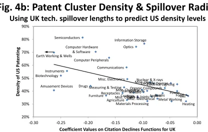
Figure 4b provides a cross-sectional plot of US cluster density against UK citation decay rates. The vertical axis is the same as Figure 4a, but we substitute the UK citation decay rates for the horizontal axis’s measure of technology spillover ranges. The UK has an outlier, raw decay rate of -0.507 (Earth Working & Wells); we cap this rate at the second-highest decay rate. There are some material adjustments among some information technology industries in Figure 4b compared to Figure 4a, with most noticeably semiconductors’decay rate not being as steep as we measured in the US. Nevertheless, a close connection exists between the decay rates for technologies in the UK and associated cluster density in the United States. The slope of the trend line is -0.979 (0.293); it is even sharper at -0.466 (0.115) when capping the US density ratio at 50%. The slope of the trend line is -0.745 (0.158) without the cap for Earth Working & Wells. These patterns provide con…dence that these relationships are not being solely determined by unmodeled factors.

Table 2 continues these analyses of single predictions regarding the size and shape of clusters. Each entry in the table is from a separate regression where the outcome variable is indicated in the column header, and the …ve panel headers indicate the metric used to model the maximal radius of interaction. Panels A and D consider the log-linear citation decay rates estimated through technique (3) measured in the US and UK, respectively. Panels B and E similarly consider the US’ and UK’s citation premium observed over 10 miles from estimation (4). Finally, Panel C models spillover lengths through the crossing points observed for technologies between …rst- and later-generation citation frequencies.

To make our estimates easily comparable to each other, we transform variables to have unit

standard deviation. We also multiply the raw j;0 10 coe¢ cient for Panels B and E by 1so that

the predicted signs for Table 2’s regressions are aligned in the same direction. These regressions exploit variation across the 36 technologies, and we control for the size of the technology using its patent count during the 1975-2009 period. Regressions are unweighted and report robust standard errors. We …nd very similar patterns when weighting technologies by size.

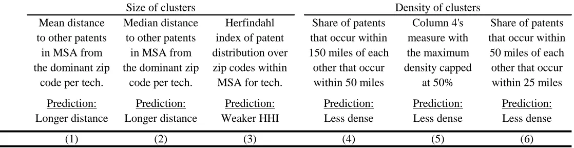
The …rst three columns examine the size of clusters, where we have the prediction that a longer maximal spillover radius produces a larger cluster. We take metropolitan statistical areas (MSAs) as the unit of observation, measuring the patenting that occurs within the zip codes of each MSA. In the next section we consider more ‡exible techniques that do not depend upon MSA de…nitions, as technology clusters may extend past MSA boundaries or across MSAs. This simple starting point is attractive, however, as it does not depend upon the structure of the continuous density techniques.

is a positive relationship in Columns 1 and 2, such that a one standard-deviation increase in the estimated maximal radius of a technology is associated with a 0.24-0.58 standard-deviation increase in these mean and median distances when using US-based radii in Panels A-C. The estimated elasticity is 0.11-0.43 when using UK-based radii in Panels D and E. Overall, with the exception of weaker performance in Panel E, these results highlight that a greater spillover range for a technology is associated with longer mean and median distances within MSAs for the technology’s patents.

Column C evaluates an alternative metric where we calculate the normalized Her…ndahl index of patents over the zip codes in a given MSA by technology. A second way that we might observe a greater size of technology clusters within a given MSA is if the patents for the technology are spread out over more zip codes (a weaker Her…ndahl index). This prediction connects with our radii as measured in Panels A and B, with very strong elasticities of about -0.63 to -0.73, and with the UK log-linear decay function in Panel D, with a strong elasticity of -0.36. On the other hand, the support in Panels C and E is weak. The coe¢ cient elasticity retains the predicted sign, but the results are not statistically signi…cant.

Columns 4-6 shift the focus towards the prediction that clusters with longer spillover radii will be less dense. Column 4 continues with the density metric examined in Figures 4a and 4b, where we measure the fraction of bilateral distances between patents that are 150 miles or less apart that are in fact 50 miles or less apart (i.e., count of patents with bilateral distances of 50 miles or less / count of patents with bilateral distances of 150 miles or less). This prediction …nds support with all of our metrics. After controlling for the size of technology, the estimated elasticity using US-based radii is 0.25-0.85; the UK-based elasticities are 0.30-0.48. These elasticities are precisely measured. Column 5 shows comparable results when capping density at 50%, and Column 6 shows similar patterns when we instead consider the density among patents that are 50 miles or less apart by looking at the fraction of these patents that are 25 miles or less apart.

5

Continuous Density Estimations

5.1

Duranton and Overman (2005)

Our empirical work in large part uses a slight variant of the Duranton and Overman (2005, hereafter DO) metric or its underlying smoothed kernel density. This discussion summarizes the DO methodology to show the connection to our theory. The empirical appendix in our NBER working paper further describes the DO metric and the empirical modi…cations required for our speci…c datasets.

The DO metric considers bilateral distances among establishments in an industry. The central calculation is the spatial density of an industry A through a continuous function:

^

KA(d) =

1

hNA_(NA ₁₎ NA ₁

X

i=1

NA

X

i0_=i+1

f d dj(i);j(i0)

h : (5)

Here, as in our basic model set-up, dj(i);j(i0₎ is the Euclidean distance between the spatial

lo-cations of establishments j(i) and j(i0_{) within industry A. The double summation considers}

every pairwise bilateral distance within the industry analyzed (i.e., NA(NA 1)=2 distances).

Establishments receive equal weight, and the function f is a Gaussian kernel density function

with bandwidth hthat smooths the series.

The resulting density function provides a distribution of bilateral distances for establishments within an industry. Across all potential distances— ranging from …rms being next door to each other to being across the country from each other— this distribution sums to1. Smoothed density functions are calculated separately for each technology or industry analyzed. Industries where establishments tend to pack together tightly in cities, for example, are measured to have higher densitiesK^A(d) at short distance ranges.

While the density function is of direct interest, it is also important to compare the observed distributions of bilateral distances to general activity in the underlying economy. This compari-son provides a basis for saying whether an industry’s spatial concentration at a given distance is abnormal or not. Because the density functions for small industries with fewer plants are natu-rally more lumpy, these comparisons are speci…c to industry size. Operationally, comparisons are calculated through 1000 random draws of hypothetical industries of equivalent size to the focal

industry A and repeating the density estimation. This procedure, which is further discussed in

the working paper’s empirical appendix, provides 5%/95% con…dence bands for each industry and distance that we designate as K_ALCI U(d) and K_ALCI L(d).

Industry localization A and dispersion Aat distanced are de…ned using the DO formulae:

A(d) max h

^

KA(d) K_ALCI U(d);0 i

(6)

A(d) max h

K_ALCI L(d) K^A(d);0 i

if A(d) = 0

and 0 otherwise.