Efficiency and Betweenness Centrality of Graphs and some Applications

RIT Scholar Works

Theses

Thesis/Dissertation Collections

2-9-2015

Efficiency and Betweenness Centrality of Graphs

and some Applications

Bryan Ek

Follow this and additional works at:

http://scholarworks.rit.edu/theses

This Thesis is brought to you for free and open access by the Thesis/Dissertation Collections at RIT Scholar Works. It has been accepted for inclusion in Theses by an authorized administrator of RIT Scholar Works. For more information, please [email protected].

Recommended Citation

Centrality of Graphs and some

Applications

by

B

ryan

E

k

A Thesis Submitted in Partial Fulfillment of the Requirements

for the Degree of Master of Science in Applied Mathematics

School of Mathematical Sciences, College of Science

Rochester Institute of Technology

Rochester, NY

Dr. Darren Narayan

School of Mathematical Sciences

Thesis Advisor

Date

Dr. Jobby Jacob

School of Mathematical Sciences

Committee Member

Date

Dr. Paul Wenger

School of Mathematical Sciences

Committee Member

Date

Dr. Rigoberto Florez

The Citadel

Committee Member

Date

Nathan Cahill, D.Phil.

School of Mathematical Sciences

Director of Graduate Programs

Abstract

The distance dG(i,j)between any two vertices i and j in a graph G is the minimum number of edges in a path between i

and j. If there is no path connecting i and j, then dG(i,j) =∞. In 2001, Latora and Marchiori introduced the measure

of efficiency between vertices in a graph. The efficiency between two vertices i and j is defined to be∈_i,j= 1

dG(i,j) for

all i6=j. The global efficiency of a graph is the average efficiency over all i6=j. The power of a graph Gmis defined to be V(Gm_{) =V(G)and E(G}m_{) ={(u,v)|d}

G(u,v)≤m}. In this paper we determine the global efficiency for path

power graphs Pnm, cycle power graphs Cmn, complete multipartite graphs Km,n, star and subdivided star graphs, and the

Cartesian products Kn×Pmt, Kn×Cmt , Km×Kn, and Pm×Pn.

The concept of global efficiency has been applied to optimization of transportation systems and brain connectivity. We

show that star-like networks have a high level of efficiency. We apply these ideas to an analysis of the Metropolitan

Atlanta Rapid Transit Authority (MARTA) Subway system, and show this network is 82% as efficient as a network

where there is a direct line between every pair of stations. From BOLD fMRI scans we are able to partition the brain

with consistency in terms of functionality and physical location. We also find that football players who suffer the largest

number of high-energy impacts experience the largest drop in efficiency over a season.

Latora and Marchiori also presented two local properties. The local efficiency E_loc= 1_{n ∑}

i∈V(G)

E_glob(Gi)is the average of

the global efficiencies over the subgraphs Gi, the subgraph induced by the neighbors of i. The clustering coefficient of a

graph G is defined to be CC(G) = 1_n∑

i

Ciwhere Ci=|E(Gi)|/(|V(2Gi)|)is a degree of completeness of Gi. In this paper,

we compare and contrast the two quantities, local efficiency and clustering coefficient.

Betweenness centrality is a measure of the importance of a vertex to the optimal paths in a graph. Betweenness centrality

of a vertex is defined as bc(v) =_∑x,yσxy(v)

σxy whereσxyis the number of unique paths of shortest length between vertices

x and y. σxy(v)is the number of optimal paths that include the vertex v. In this paper, we examined betweenness

centrality for vertices in Cm

n. We also include results for subdivided star graphs and C3star graphs.

A graph is said to have unique betweenness centrality if bc(vi) =bc(vj)implies i= j: the betweenness centrality

function is injective over the vertices of G. We describe the betweenness centrality for vertices in ladder graphs, P2×Pn.

An appended ladder graph Unis P2×Pnwith a pendant vertex attached to an “end”. We conjecture that the infinite

C

ontents

I Introduction 1

I.1 Efficiency . . . 1

I.2 Betweenness Centrality . . . 2

I.3 Definitions . . . 3

II Global Efficiency 5 II.1 Definition and Example . . . 5

II.2 Path Graphs: Pn . . . 6

II.3 Path Power Graphs: Pm n . . . 7

II.4 Cycle Power Graphs: Cm_n . . . 9

II.5 Complete Multipartite Graphs . . . 12

II.6 Efficiency under the Euclidean Metric . . . 14

II.7 Uniformly Subdivided Star Graphs: Sd,l . . . 15

II.7.1 Weighted Efficiencies . . . 18

II.7.2 New Unweighted Global Efficiency and Double Sum Reduction . . . 22

II.8 Cartesian Products . . . 22

II.8.1 Kr×Pnm . . . 23

II.8.2 Kr×Cmn . . . 25

II.8.3 Km×Kn . . . 27

II.8.4 Grid Graphs:Pm×Pn . . . 29

II.8.5 Harary Index . . . 33

II.9 Applications . . . 34

II.9.1 Metropolitan Atlanta Rapid Transit Authority Subway . . . 34

II.9.2 Brain Network . . . 37

III Local Efficiency and Clustering Coefficient 40 III.1 Graphs where the Clustering Coefficient and Local Efficiency Differ . . . 40

III.1.1 Clustering Coefficients vs. Local Efficiency for Complete Multipartite Graphs . . . 40

III.1.2 Cycle Powers . . . 42

III.1.3 Networks of the Brain . . . 45

III.2 Graphs whereCandElocare equal . . . 46

III.2.1 Clustering Coefficients vs. Local Efficiency for Cartesian Products of Graphs . . . 46

III.3 Summary of Differences in Local Efficiency and Clustering Coefficient . . . 46

IV Betweenness Centrality 48 IV.1 Introduction . . . 48

IV.1.1 Definition and Example . . . 48

IV.1.2 Bounds on Betweenness Centrality . . . 48

IV.2 Betweenness Centrality for Various Graphs . . . 49

IV.2.1 Cycle Powers . . . 49

IV.2.2 Subdivided Star Graphs . . . 51

IV.2.3 Subdivided Triangle Star Graphs . . . 51

IV.2.4 Ladders . . . 51

IV.2.5 Pendant Ladders . . . 53

IV.3 Unique Betweenness Centrality . . . 54

IV.3.1 Necessary Conditions . . . 54

IV.3.2 Infinite Family of Graphs with Unique Betweenness Centrality . . . 55

V Future Research 61 VI Conclusion 62 VI.1 Efficiency . . . 62

VI.2 Betweenness Centrality . . . 63

VII Acknowledgments 64 VIII Appendix 65 VIII.1 Efficiency . . . 65

VIII.1.1Sum Simplifications . . . 65

VIII.1.2Faster Efficiency Formulae . . . 66

VIII.1.3MARTA . . . 71

VIII.1.4Brain Network . . . 74

VIII.2 Betweenness Centrality . . . 76

VIII.2.1Unique Betweenness Centrality Lemmas and Table . . . 76

I.

I

ntroduction

I.1

Efficiency

In this thesis, we are concerned with several measures of connectivity of graphs: global efficiency, local efficiency, clustering coefficient and betweenness centrality.

In 2001, Latora and Marchiori introduced the measure of efficiency between vertices in a graph [1]. The (unweighted)efficiencybetween two verticesvi andvj is defined to be∈ (vi,vj) = _d(v1

i,vj) for alli6= j. The

global efficiencyof a graphEglob(G) = _n(n1₋₁₎∑i6=j∈(vi,vj)which is simply the average of the efficiencies over

all pairs of the distinctnvertices. Then note that 0≤Eglob(G)≤1 with equality only when Ghas no edges

and whenGis a complete graph respectively.

The concept of reciprocal distance has been studied previously. In 1993, Plavši´c, Nikoli´c, Trinajsti´c, and Mihali´c introduced theHarary indexof a simple graph [2]. For a simple graphGwith verticesv1,v2, ...,vnthe Harary

index is denotedH(G)and equals ∑

1≤i<j≤n

1

d(vi,vi). We note the close relationship between global efficiency and

the Harary index,Eglob(G) = _n(n2−1)H(G). There also have been other studies involving the Harary index and reciprocal distances [3, 4, 5, 6, 7].

In this thesis we determine the global efficiency for path power graphsPnm, cycle power graphsCmn, complete

multipartite graphs Km,n, star and subdivided star graphs, and the Cartesian ProductsKn×Pmt,Kn×Ctm, Km×Kn, and Pm×Pn. As a consequence, we determine new results involving the Harary index for these

families of graphs.

Recently other papers have studied the concept of efficiency, [8, 9, 10, 11, 12]. A comprehensive analysis of all of these measures is given by Sporns [13].

level of efficiency. We apply these ideas to an analysis of the MARTA Subway system and show that their network is 82% as efficient as a network where there is a direct line connecting each pair of stations.

Latora and Marchiori also presented two local properties[8]. Thelocal efficiency Eloc = n1 ∑ i∈G

Eglob(Gi)is the

average of the global efficiencies over the subgraphs Gi, the subgraph induced by the neighbors ofi. The clustering coefficientof a graphGis defined to beCC(G) = _n1_∑

i

Ci whereCi =|E(Gi)|/(|V(₂Gi)|)is a degree of

completeness ofGi. In this thesis, we compare and contrast the two quantities, local efficiency and clustering

coefficient. We include results of these local measurements for complete multipartite graphsKn,m, cycle power

graphsCnm, and Cartesian productsKm×Kn andKn×Cm.

RCBI scientists conducted functional MRI (fMRI) scans of 25 volunteers to find blood oxygen level-dependent (BOLD) correlations of various regions of the brain. We constructed graphs with edges based on correlation cutoffs and then partitioned the brain using efficiency. The partitions were found to be consistent with functionality and physical location within the brain. We also used these measurements to analyze the effects of a season of hard-contact football on University of Rochester athletes. Again, an outside source conducted BOLD pre and postseason fMRI scans of the players. We received matrices of the correlations in oxygen levels of various regions of the brain and modeled these as graphs. We were then able to measure the “efficiency” of each athlete. As was expected, the athletes who received the largest number of high-energy impacts during the season also experienced the largest drop in brain efficiency. For comparison, we calculated the measurements of a macaque brain using data (see Figure VIII.1.1) from Honey et al.[12]

It was stated by Latora and Marchiori [1] that “It can be shown that, when in a graph, most of its local subgraphsGi are not sparse, thenC[clustering coefficient] is a good approximation ofEloc. In summary, there

are not two different types of analyses to be done for the global and local scales, just one with a very precise physical meaning: the efficiency in transporting information”. Due to the vague wording of “not sparse” we provide an in-depth analysis of this statement, identifying graphs where the clustering coefficient and local efficiency are in fact non-negligibly different. We also identify certain graph families where the two quantities are the same.

I.2

Betweenness Centrality

Betweenness centrality is a measure of the importance of a vertex to the optimal paths in a graph. Betweenness centrality of a vertex is defined asbc(v) =_∑x,yσxy(v)

length between verticesx andy.σxy(v)is the number of optimal paths that include the vertexv. In this thesis,

we examined betweenness centrality for vertices inCm

n. By the symmetry ofCmn, every vertex will have the

same betweenness centrality. We also include results for subdivided star graphs andC3star graphs.

A graph is said to have unique betweenness centrality if bc(vi) = bc(vj) implies i = j: the betweenness

centrality function is injective over the vertices ofG. We describe the betweenness centrality for vertices in ladder graphs,P2×Pn. An appended ladder graphUnisP2×Pnwith a pendant vertex attached to an “end”.

We conjecture that the infinite family of appended graphs has unique betweenness centrality. We were able to construct a partial proof but were forced to leave the completion as future research.

I.3

Definitions

Definition I.3.1. Agraph,G, is a collection of a set of vertices,V(G), and a set of edges,E(G). The graph can be denotedG(V,E). An edge is an unordered pair of vertices. Thedistance dG(i,j)between any two vertices iandjin a graph Gis the minimum number of edges in a path betweeniandj. The subscript notation is dropped if it is apparent with respect to which graph the distance is. If there is no path connectingiandj,G

is disconnected, thend(i,j) =∞.

Definition I.3.2. The power of a graph, G, denoted Gm, is defined to be V(Gm) = V(G) and E(Gm) = {(u,v)|dG(u,v)≤m}. With this definitionG1=G.

Definition I.3.3. Given a graphGand a vertexv∈V(G), theneighborhood subgraph induced by vis the subgraph containing all vertices adjacent tovand all edges, if any, that may exist between the adjacent vertices.

Definition I.3.4. Theeccentricityof a vertexvin a graphGis defined ase(v) =max{d(v,u)|u∈V(G)}. The

diameterof a graph,G, is defined asdiam(G) =max{e(v)|v∈V(G)}. Diameter is the largest distance between two vertices in the graph.

Remark I.3.5. Note thateand∈are separate symbols and∈(x,y)denotes the efficiency between verticesx

andyand∈alone means contained in, as in “an element is contained in a set”.

Remark I.3.6. When we mention a “step” in paths of graphs, we mean an intermediate vertex of the path.

useful for simplifications. Note that for ease of use, we defineH0=0.

Definition I.3.8. Anautomorphism of a graph G(V,E) is a bijective (one-to-one and onto) function on the vertices ofG,φ:V→V, that preserves edges. i.e. φis a permutation ofVthat preserves edges. Preserving

edges means that(v1,v2)∈ E(G)if and only if(φ(v1),φ(v2))∈E(G(φ(V),E)). The set of automorphisms is

denoted Aut(G)and forms a group under composition[14].

Definition I.3.9. LetHbe a group of permutations of a setS. For eachs∈ S, let orbH(s) ={φ(s)|φ∈ H}.

orbH(s)is called theorbitofsunderH. The orbits partitionSinto equivalence classes[15].

Definition I.3.10. Let G(V,E) be a graph. Gis said to bevertex-transitive if for all u,v ∈ V, we have that

u∈orb_Aut(G)(v)(or equivalentlyv∈orb_Aut(G)(u)). i.e. there exists someφ∈ Aut(G)such thatφ(v) =u(or

II.

G

lobal

E

fficiency

II.1

Definition and Example

Definition II.1.1. Consider a graphGof ordern. Theglobal efficiencyis defined as

Eglob(G) =

1

n(n−1)_i

∑

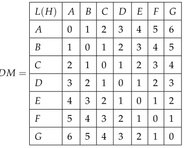
where∈(vi,vj) = _d(v1_i,vj). The global efficiency is the average efficiency of all pairs of vertices. Example II.1.2. LetH=P7with verticesA,B,C,D,E,FandG. See Figure II.1.1.

A B C D E F G

Figure II.1.1:P7for efficiency example.

The distances between each pair of vertices is given in the matrix shown below.

DM=

L(H) A B C D E F G

A 0 1 2 3 4 5 6

B 1 0 1 2 3 4 5

C 2 1 0 1 2 3 4

D 3 2 1 0 1 2 3

E 4 3 2 1 0 1 2

F 5 4 3 2 1 0 1

G 6 5 4 3 2 1 0

Definition II.1.3. The average distance,D(H), between vertices in a graphHshall be denoted:

D(H) = 1

n(n−1)

∑

The inverse ofD(H)is a first approximation of the global efficiency.

In this case,D(P7) = ₇2·6[6(1) +5(2) +4(3) +3(4) +2(5) +1(6)] = 83. The first approximation of the global

The efficiency matrix is then as follows.

EM=

E(H) A B C D E F G

A 0 1 1₂ 1₃ 1₄ 1₅ 1₆

B 1 0 1 1₂ 1₃ 1₄ 1₅

C 1₂ 1 0 1 1₂ 1₃ 1₄

D 1₃ 1₂ 1 0 1 1₂ 1₃

E 1₄ 1₃ 1₂ 1 0 1 1₂

F 1₅ 1₄ 1₃ 1₂ 1 0 1

G 1₆ 1₅ 1₄ 1₃ 1₂ 1 0

We note that the matrix is symmetric about the main diagonal. We can also sum the elements in the upper triangle of the matrix: 6(1) +5(1₂) +41₃+31₄+21₅+11₆. Finally we divide by the number of

non-diagonal elements. ThereforeEglob(P7) = ₇1·6·2 ₇₋₁

∑

i=1 7−i

i

= 223₄₂₀ ≈0.531. The first approximation in this case is off by nearly 30%: not very good.

II.2

Path Graphs:

P

LetPndenote the path on verticesv1,v2, ...,vn with edgesv1v2,v2v3, ...,vn−1vn. The distanced(vi,vj)between

distinct verticesvi andvjis|i−j|. Hence the efficiency betweenvi andvjis∈(vi,vj) = _d(v1_i,vj) = |i−1j|.

Theorem II.2.1.

Eglob(Pn) =2

Hn−1

n−1 − 1

n

. (II.2.1)

Proof. Consider the paths of various lengths inPn. Without loss of generality we assume the “starting” vertex

is located to the left of the ending vertex. Note that this will only account for half of the efficiencies. If we want to moveivertices to the right there are onlyn−istarting vertices. Hence for the efficiency matrix of

Pn, there aren−ipairs of vertices whose efficiency is 1_i. Then by doubling our efficiencies since the matrix

is symmetric, and then normalizing, we haveEglob(Pn) = _n·(n2₋₁₎

_n−1

∑

i=1

n−i i

. Simple algebraic manipulation yields the theorem.

Theorem II.2.2.

lim

n→∞Eglob(Pn) =0

Proof. Using Lemma VIII.2.1,

0≤ lim

n→∞Eglob(Pn) =nlim→∞

2

Hn−1

n−1 − 1

n

=2 lim

n→∞

Hn−1

n−1−2 limn→∞ 1

n

≤2 lim

n→∞

ln(n−1) +1

n−1 −2 limn→∞ 1

n

=2 lim

n→∞

ln(n−1)

n−1 +2 limn→∞ 1

n−1−2 limn→∞ 1

n

=0+2 lim

n→∞ 1

n−2 limn→∞ 1

n

=0.

II.3

Path Power Graphs:

P

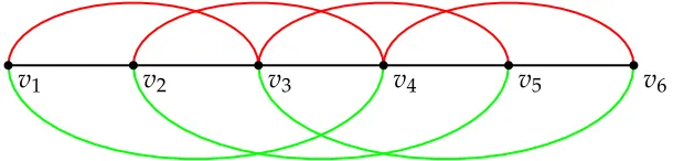
We next investigate the efficiency of powers of a pathPn. Su, Xiong, and Gutman obtained the Harary index of P_nm, from whichEglob(Pnm)can easily be obtained. However, we include a computation ofEglob(Pnm), as it is

useful for obtaining the global efficiency for the familiesKn×PnmandKn×Cnm.

v

v

v

v

v

v

Figure II.3.1:A representation of the path power: P3 6.

For the global efficiency of path power graphs: Eglob(Pnm), each element of the efficiency matrix is given

by

∈_ij= l_|i−1_j|

m

whereiis the row andjis the column of the entry. This value corresponds to the efficiency between verticesi

andj. The distance between the vertices inPn is simply|i−j|. InPnm, each step can be up tomvertices away.

Hence the distance between vertices equalsl|i−_mj|m. Taking the inverse gives the formula in Eq. (II.3.1). Hence the matrix is:

v1 v2 v3 · · · vn−2 vn−1 vn

v1 0 1 1 _dn−13

m e

1 dn−2

m e

1 dn−1

m e

v2 1 0 1 · · · _dn−14

m e

1 dn−3

m e

1 dn−2

m e

v3 1 1 0 _dn−15

m e

1 dn−4

m e

1 dn−3

m e

..

. ... . .. ...

vn−2 _dn1−3

m e

1 dn−4

m e

1 dn−5

m e

0 1 1

vn−1 _dn1−2

m e

1 dn−3

m e

1 dn−4

m e

· · · 1 0 1

vn _dn1−1

m e

1 dn−2

m e

1 dn−3

m e

1 1 0

Consider the first vertex ofPnm. There are(n−1)other vertices to compute the efficiency with. The sum of

efficiencies from the first vertex is:

n

∑

j=2 ∈1,j=

n

∑

j=2

1

l_|1−j|

m

m =

n−1

∑

i=1

1

l

i m

m.

For the second vertex we have, 1≤ |2−j| ≤n−2 since 3≤j≤n, which yields:

n

∑

j=3 ∈_2,j=

n

∑

j=3

1

l_|2−j|

m

m =

n−2

∑

i=1

1

l

i m

m.

Summing the terms for all vertices gives:

n−1

∑

i=1

1

l

i m

m+

n−2

∑

i=1

1

l

i m

m+· · ·+ 2

∑

i=1

1 l i m m+ 1

∑

i=1

1

l

i m

m =

n−1

∑

i=1

n−i

l

i m

m.

Finally, we divide this term to get the result of Theorem II.3.1. We note as the matrix is symmetric, we can sum over the upper half of the matrix (ordered pairs) and then multiply our result by 2. The last step is normalization.

Theorem II.3.1.

Eglob(Pnm) =

2

n(n−1) n−1

∑

i=1

n−i

l

i m

m. (II.3.2)

II.4

Cycle Power Graphs:

C

Definition II.4.1. ACycle Graph Cn has verticesv1,v2, . . . ,vn and edges(vi,vj)if|i−j|=1 as well as the edge (v1,vn).

Definition II.4.2. A Cycle Power Graph Cnm has vertices v1,v2, . . . ,vn and edge (vi,vj) if and only if

1≤min(|i−j|,n− |i−j|)≤m. This condition is equivalent to 1≤n

2

−

|i−j| −n₂

≤m.

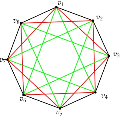
Consider the CycleC3₈:

v

v

v

v

v

v

v

v

Figure II.4.1:A representation of the power cycle:C₈3.

The efficiency matrix is given as:

v1 v2 v3 v4 v5 v6 v7 v8

v1 0 1 1 1 1₂ 1 1 1

v2 1 0 1 1 1 12 1 1

v3 1 1 0 1 1 1 12 1

v4 1 1 1 0 1 1 1 12

v5 12 1 1 1 0 1 1 1

v6 1 12 1 1 1 0 1 1

v7 1 1 1₂ 1 1 1 0 1

v8 1 1 1 1₂ 1 1 1 0

scaling it appropriately. Hence,

Eglob(C83) =

52 8(8−1) =

13

14 =0.929.

Note that rows are identical; they are merely shifted representations of each other. This is the case due to the symmetry of the cycle. The following is the generic efficiency matrix forC₂m_n.

v1 v2 · · · vi · · · vn

2 vn2+1 · · · vj · · · vn−1 vn

v1 0 1 · · · _di−11

m e

· · · 1 dn/2−1

m e

1 dn/2

m e

· · · 1

l_n+1−j

m

m · · · 1 1

.. .

vn 1 1 · · · _d1i me

· · · 1 dn/2

m e

1 dn/2+1

m e

· · · 1

l_n+2−j

m

m · · · 1 0

Also, note that each row (by removing the zero: efficiency to itself) is symmetric to itself so the sum of the row is the same as twice the first half. For even cases, the center element is counted twice, thus it must be removed once. So considering the first portion of the last row, theithelement is given as:

∈(vi,vn) =l1

i m

m.

So the sum of the row is almost given by:

2

n

2

∑

i=1

1

l

i m

m.

As indicated above, the center element is incorrectly doubled; however, the above sum does not take this into account. As a result, _d1n

2me

must be subtracted off. The total efficiency is then the row sum multiplied by the number of rows:n. Therefore the global efficiency of any power cycle with an even number of vertices:n, is given by:

Lemma II.4.3. For even n,

Eglob(Cnm) =

1

n(n−1)

 n  2 n 2

∑

i=1

1 l i m m− 1 _n 2m     = 1

(n−1)



2

n

2

∑

i=1

1 l i m m− 1 _n 2m 

. (II.4.1)

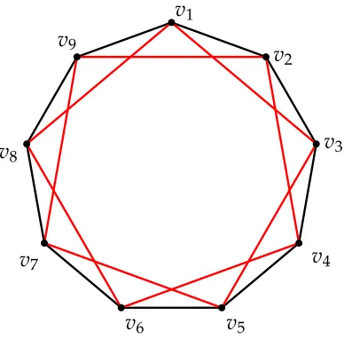
v

v

v

v

v

v

v

v

v

Figure II.4.2:A representation of the power cycle:C₉2.

The efficiency matrix is given as:

v1 v2 v3 v4 v5 v6 v7 v8 v9

v1 0 1 1 1₂ 1₂ 1₂ 1₂ 1 1

v2 1 0 1 1 12 12 12 12 1

v3 1 1 0 1 1 1₂ 1₂ 1₂ 1₂

v4 12 1 1 0 1 1 12 12 12

v5 12 12 1 1 0 1 1 12 12

v6 1₂ 1₂ 1₂ 1 1 0 1 1 1₂

v7 12 12 12 12 1 1 0 1 1

v8 1 1₂ 1₂ 1₂ 1₂ 1 1 0 1

v9 1 1 1₂ 1₂ 1₂ 1₂ 1 1 0

From the efficiency matrix,

Eglob(C29) =

9(1+1+1₂+1₂+1₂+1₂+1+1)

9(9−1) =

9·6 9·8 =

3

The generic efficiency matrix forCm

n, wherenis odd, is then given by:

v1 v2 · · · vi · · · vn+1

2 vn

+1

2 +1 · · · vj · · · vn−1 vn

v1 0 1 · · · _di−11

m e

· · · 1

l_(n−1)/2

m

m l_(n−1_1)/2

m

m · · · l_n+1_1−j

m

m · · · 1 1

.. .

vn 1 1 · · · _d1i me

· · · 1

l_(n−1)/2

m

m l_(n−1_3)/2

m

m · · · l_n+1_2−j

m

m · · · 1 0

Considering the first portion of the first row, theithelement is given as:

∈(vi,v1) = l 1

i−1

m

m.

So the sum of the row is given by:

2

n+1 2

∑

i=2

1

l

i−1

m

m =2

n−1 2

∑

i=1

1

l

i m

m.

Note the sums are identical; the index was merely shifted. And so the global efficiency forCnm, wherenis odd,

is found by multiplying this sum by the number of rows and normalizing:

Lemma II.4.4. For odd n,

Eglob(Cnm) =

2

(n−1)

n−1 2

∑

i=1

1

l

i m

m. (II.4.2)

We can combine Lemmas II.4.3 and II.4.4 into Theorem II.4.5.

Theorem II.4.5.

Eglob(Cmn) =

  

 

1 2k−1

∑k i=1_d2i

me

− 1 dk me

if n=2k,

1

k∑ k i=1_d1i

me

if n=2k+1.

(II.4.3)

An alternate formula for faster computation can be found in Corollary VIII.1.6.

II.5

Complete Multipartite Graphs

Definition II.5.1. Acomplete multipartite graph G = Ks1,s2,...,st is composed oft classes each withsi vertices,

1≤i≤t, where each vertex in classiis adjacent to every vertex in classj6=i, and is not adjacent to any vertex in classi.

Theorem II.5.2. Let G=Ks1,s2,...,st, t>1, and let n=∑

t

i=1si. Then

Eglob(G) =1− 1

2(n−1)

"

1

n t

∑

i=1

s2_i −1

#

. (II.5.1)

Proof. Letvbe a vertex in a part withsivertices. Then the shortest path fromvto any vertex in the same part

is 2 andvis adjacent to all vertices in other parts. Hence for every vertex,v, in parti, the sum of efficiencies including v ish(si−1)

2 + (n−si)

i

. Summing over all vertices in a given part and then over all parts gives

t

∑

i=1v∈part∑ i

h_(s

i−1)

2 + (n−si)

i

= ∑t i=1

si

h_(s

i−1)

2 + (n−si)

i

. Normalizing and some algebraic manipulation gives the desired result.

Remark II.5.3. If we increase the value ofn, the efficiency doesn’t necessarily tend toward 1. It all depends on the distribution of vertices within the classes. If one class is filled with nearly all the vertices, then the efficiency will tend towards 1₂. Other ratios will tend toward different values in between 1₂ and 1.

For the small case oft=2,s1=n,s2=m: complete bipartite graphs, we have great simplifications.

Theorem II.5.4.

Eglob(Kn,m) =1− 1

2(n+m−1)

_n2_+m2

n+m −1

. (II.5.2)

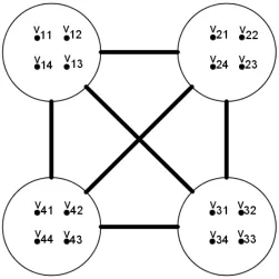
Another simplification due to symmetry is forKr,...,r: a complete multipartite graph withnclasses, each withr

vertices. We will denote the complete multipartite graphKr,...,r asKr;n. An example is shown below in Figure

Figure II.5.1:A complete multipartite graph.K4;4

Theorem II.5.5.

Eglob(Kr;n) =1− r −1

2(nr−1). (II.5.3)

Remark II.5.6. As the number of classes increases, the complete multipartite graph begins to approach the appearance of a complete graph. Thus we have a global efficiency approaching 1.

lim

n→∞Eglob(Kr;n) =1.

Increasing the number of vertices in each class tends to decrease the global efficiency since this increases the number of optimal paths of length 2 (the worst paths). However it also increases the number of optimal paths of length 1 depending on the number of classes. Thus we arrive at a lower bound for the global efficiency based on the number of classes.

lim

r→∞Eglob(Kr;n) =1− 1 2n.

II.6

Efficiency under the Euclidean Metric

the latter as maximum weighted efficiency. In calculating the maximum weighted efficiency, we consider every pair of vertices to be adjacent with the weight of an edge as the Euclidean distance between the corresponding vertices. Note then that the weighted efficiency is highly dependent on the orientation of the graph as well as the plane in which it is embedded.

a

b

c

Figure II.6.1:Demonstration of the effect of considering Euclidean distance.

For the unweighted efficiency we have ∈ (x,y) = 1, ∈ (x,z) = 1, and∈ (y,z) = 1₂. Hence Eglob(G) =

1

3·2·2(1+1+12) = 56 ≈0.83. However for the maximum weighted efficiency we have∈(x,y) =1,∈(x,z) =1,

and∈(y,z) = √1

2. HenceE

w

glob(G) = 31·2·2(1+1+√12) = 1 6

√

2+2₃≈0.90.

In Figure II.6.1, we compare the two types of efficiency of the graphG, drawn with a prescribed orientation. By examining the ratio of the unweighted efficiency to the maximum weighted efficiency, we can compare how efficient a graph network is compared to a Euclidean network. The ratioERatio(G) =Eglob(G)/Ewglob(G) = 56/(

1 6

√

2+2₃)≈0.92. Hence for the particular graph in Figure II.6.1, the graph is 92% as efficient as the completed graph under the Euclidean metric.

The case whereG=Pnis straightforward since the shortest distance between any points is a straight line. This

assumes that the path is oriented in the “usual” fashion of a line. Hence

Theorem II.6.1. Eglob(Pn) =Ew_glob(Pn), and ERatio(Pn) =1.

II.7

Uniformly Subdivided Star Graphs:

S

In this subsection we consider the efficiency of star-like networks. The graphK1,r is called a star and is a

Definition II.7.1. Anedge subdivisionis an operation that is applied to an edgeuvwhere a new vertex w is inserted, and the edgeuvis replaced by edgesuwandwv. Asubdivision Hof a graphGis a graph that can be obtained by performing a sequence of edge subdivisions.

Hence we can define a subdivided star.

Definition II.7.2. LetSd,l be the subdivision of the star K1,r where each edge is replaced by a path with l

vertices. The vertex of degreedwill be referred to as the center.

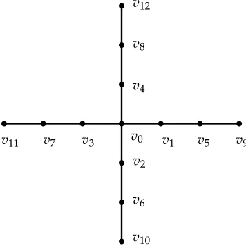
The subdivided starS4,3is shown in Figure II.7.1.

v2

v3

v4

v5

v6

v7

v8

v9

v10

v11

v12

v0 _v1

Table II.7.1:Efficiency matrix forS(4, 3).

v0 v1 v2 v3 v4 v5 v6 v7 v8 v9 v10 v11 v12

v0 0 1 1 1 1 1₂ 1₂ 1₂ 1₂ 1₃ 1₃ 1₃ 1₃

v1 0 12 12 12 1 13 13 13 12 14 14 14

v2 0 1₂ 1₂ 1₃ 1 ₃1 1₃ 1₄ 1₂ 1₄ 1₄

v3 0 1₂ 1₃ 1₃ 1 1₃ 1₄ 1₄ 1₂ 1₄

v4 0 13 13 13 1 14 14 14 12

v5 0 1₄ 1₄ 1₄ 1 1₅ 1₅ 1₅

v6 0 14 14 15 1 15 15

v7 0 14 15 15 1 15

v8 0 1₅ 1₅ 1₅ 1

v9 0 16 16 16

v10 0 1₆ 1₆

v11 0 16

v12 0

We first examine efficiencies between vertices on the same spoke including the center. Note that based on our labeling, there are three blocks of four identical entries across the top row and each continues in a “downward diagonal pattern”. The total sum of these diagonals is: 4(₁3)+4(₂2)+4(₃1).

Next we examine efficiencies between vertices on different spokes. There are “patches” of(4₂) =6 identical entries. There is one patch where the entries are equal to 1₂, two patches where the entries equal 1₃, three patches where the entries equal 1₄, two patches where the entries equal 1₅, and one patch where the entries equal 1₆. This pattern is inherent from the labeling of our vertices. The verticesvhi+1,vhi+2,vhi+3,vhi+4, all have

distancehfrom the center. We will consider paths between vertices on different spokes. Paths of length 2 must be between vertices whereh=1. Paths of length 3 must be between vertices where one vertex hash=1 and another hash=2. Paths of length 4 must be between vertices where both vertices haveh=2, or where one hash=1 and the other hash=3. Paths of length 5 must be between vertices where one vertex hash=2 and another hash=3. Paths of length 6 must be between vertices whereh=3. For each partition of a path length, there will be(4₂)paths: picking the spokes to travel between.

The sum over all of the patches is 4(₂3)·1 2+

4(3)

2 · 23+ 4(3)

2 ·34+ 4(3)

2 · 25+ 4(3)

main diagonal, the total sum over all efficiencies is

2·

4(3)

1 + 4(2)

2 + 4(1)

3 + 4(3)

2 · 1 2+

4(3)

2 · 2 3+

4(3)

2 · 3 4 +

4(3)

2 · 2 5 +

4(3)

2 · 1 6 = 967 15. Dividing by the number of non-diagonal entries in our matrix gives: ₁₃1_·12· 967

15 = 2340967 =0.413 25.

This example provides the structure for the proof of our next theorem.

Theorem II.7.3. We have

Eglob(Sd,l) = 2 l(dl+1)

(d−1)

l+1

2

H2l−(d−2)(l+1)Hl−l

. (II.7.1)

Proof. First we consider the efficiencies between vertices on the same spoke including the center. Each spoke is isomorphic toPl+1. By Theorem II.2.1 the sum of the efficiencies of this spoke is(l+1)Hl−l. Hence the total

sum of the efficiencies over alldspokes isd[(l+1)Hl−l].

Next we consider efficiencies between vertices on different spokes. In general the number of paths of lengthk

inSd,l will equal the number of partitions ofkintoaandbwherea,b≤l. Each partitionk=a+bcorresponds

to a path inSd,l that travels through the center with a subpath of lengthafrom the starting vertex to the center

and a subpath of lengthbfrom the center to the end vertex. These correspond to the patches with entries equal to 1_k.

Each of the patches will contain(d₂)identical entries since this is the number of ways to choose the starting and ending spokes. Considering the various partitions ofkthere will beipatches where all of the entries are equal to _i+1₁ for 1≤i≤landipatches where all of the entries are equal to _2l+1_1−i for 1≤i≤l−1.

The total sum is ∑l

i=1

d(d−1)

2 · i+i1+

l−1

∑

i=1

d(d−1)

2 ·2l+i1−i. The sum of the efficiencies for a subdivided star graph

withdspokes, each of lengthlis then (doubling for the symmetry of the matrix):

∑

i,j

∈ij=2 d[(l+1)Hl−l] + l

∑

i=1

d(d−1)

2 ·

i i+1 +

l−1

∑

i=1

d(d−1)

2 ·

i

2l+1−i

!

,

which can simplify to

2d

(d−1)

l+1

2

H2l−(d−2)(l+1)Hl−l

. Normalizing withn=dl+1 completes the proof.

II.7.1 Weighted Efficiencies

between any adjacent vertices to be 1. Furthermore, we consider all spokes to be linear and spaced at equal angles around the center vertex,v0in the plane. Weighted efficiency can effectively approximate real-world

networks such as a subway system. This is found by dividing the unweighted global efficiency by the maximum weighted global efficiency.

3√2

v

v

v

v

v

v

v

v

v

v

v

v

v

Figure II.7.2:AnS4,3graph partially completed.

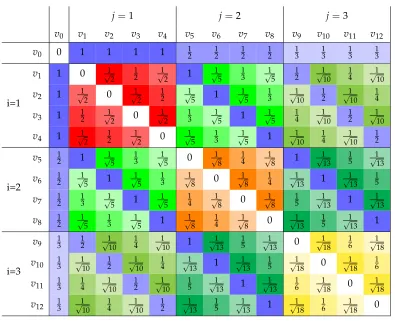
The following, Table II.7.2, is a matrix of the efficiency of a subdivided star graph as if each pair of vertices were connected with an edge weighted by the Euclidean distance between them, see Figure II.7.2. For example,

v8 andv11 would be connected by an edge of weight equal to the Euclidean distance between the points, √

22₊₃2₌√_{13. Here the efficiency∈(v}

Table II.7.2:Euclidean efficiency matrix forS(4, 3).

j=1 j=2 j=3

v0 v1 v2 v3 v4 v5 v6 v7 v8 v9 v10 v11 v12

v0 0 1 1 1 1 1₂ 1₂ 1₂ 1₂ 1₃ 1₃ 1₃ 1₃

v1 1 0 √1₂ 1₂ √1₂ 1 √1₅ 1₃ √1₅ 1₂ √1₁₀ 1₄ √1₁₀

i=1 v2 1

1

√

2 0

1

√

2 1

2 √1₅ 1 √1₅ 13 √1₁₀ 12 √1₁₀ 14

v3 1 12 √1₂ 0 √1₂ 13 √1₅ 1 √1₅ 14 √1₁₀ 12 √1₁₀

v4 1 √1₂ 1₂ √1₂ 0 √1₅ 1₃ √1₅ 1 √1₁₀ 1₄ √1₁₀ 1₂

v5 1₂ 1 √1₅ 1₃ √1₅ 0 √1₈ 1₄ √1₈ 1 √1₁₃ 1₅ √1₁₃

i=2 v6

1

2 √1₅ 1 √1₅ 13 √1₈ 0 √1₈ 14 √1₁₃ 1 √1₁₃ 15

v7 1₂ 1₃ √1₅ 1 √1₅ 1₄ √1₈ 0 √1₈ 1₅ √1₁₃ 1 √1₁₃

v8 1₂ √1₅ 1₃ √1₅ 1 √1₈ 1₄ √1₈ 0 √1₁₃ 1₅ √1₁₃ 1

v9 1₃ 1₂ √1₁₀ 1₄ √1₁₀ 1 √1₁₃ 1₅ √1₁₃ 0 √1₁₈ 1₆ √1₁₈

i=3 v10

1

3 √1₁₀ 12 √1₁₀ 14 √1₁₃ 1 √1₁₃ 15 √1₁₈ 0 √1₁₈ 16

v11 1₃ 1₄ √1₁₀ 1₂ √1₁₀ 1₅ √1₁₃ 1 √1₁₃ 1₆ √1₁₈ 0 √1₁₈

v12 13 √1₁₀ 14 √1₁₀ 12 √1₁₃ 15 √1₁₃ 1 √1₁₈ 16 √1₁₈ 0

Notice that the blocks of 4 identical terms with diagonals directed downward are identical to those appearing in the non-weighted case. These are the efficiencies between vertices on the same spoke or the center. For the pairs of vertices on different spokes, we focus on the squares which represent efficiencies between two vertices, where one is distanceifrom the center and the other is distancejfrom the center. For box,i=1 andj=2, the sum equals 8· √1

5+4· 1

3 = √4₅+43+√4₅. In Figure 5, going fromv1tov8requires a turn of an angle of π2. The

terms can be expressed using the law of cosines: 4

q

12₊₂2_{−2·1·2·cos} π

2

+_p 4

12₊₂2_{−2·1·2·cos(π)}+

4

q

12₊₂2_{−2·1·2·cos} 3π

2 .

Theorem II.7.4.

Ew_glob(Sd,l) =

1

l(dl+1)



2(l+1)H_l−2l+

l

∑

i=1

l

∑

j=1

d−1

∑

θ=1

1

q

i2_+j2_−2ijcos 2π

d θ



. (II.7.2)

lines in the Euclidean plane. We also assume that every spoke is spaced around the center vertex at equal angle intervals.

The sum of the efficiencies for vertices on the same spoke including the center is almost the same as in the proof of the previous theorem, 2d((l+1)Hl−l). We need to double this now as we are not doubling all terms

later. Next we consider the pairs of vertices that are found on different spokes. In general the number of paths of lengthkinSd,l will equal the number of partitions ofkintoaandbwherea,b≤l. Each partitionk=a+b

corresponds to a path inSd,l that travels through the center with a subpath of length afrom the starting

vertex to the center and a subpath of lengthbfrom the center to the end vertex. These form entries equal to √ 1

a2_+b2_−2abcosθ whereθis the angle between spokes. We focus on thed×d submatrices which represent

efficiencies between two vertices, where one is distanceifrom the center and the other is distancejfrom the center.

The generic terms in a givend×dsubmatrix could then be written as q d i2_+j2_−2ij·cos(2π

d θ)

whereθvaries from

1 to d−1. We then sum over all d×d submatrices and add the diagonal terms to yield the sum of the Euclidean efficiencies forSd,l, ∑

i6=j

∈ (vi,vj) = 2d((l+1)Hl−l) + l

∑

i=1

l

∑

j=1

d−1

∑

θ=1

d q

i2_+j2_−2ijcos(2π

d θ)

. Normalizing withn=dl+1 gives the result.

An alternate formula for faster computation can be found in Corollary VIII.1.7.

Instead of normalizing by the maximum number of edges, n(n−1), we can normalize by the maximum weighted efficiency. The efficiency ratio, ERatio for a subdivided star graph Sd,l is found by dividing the

unweighted global efficiency by the maximum weighted global efficiency.

Theorem II.7.5.

ERatio(Sd,l) =

(d−1) (2l+1)H2l−(d−2)(2l+2)Hl−2l (2l+2)Hl−2l+∑il=1∑lj=1∑dθ−=11

1

q

i2_+j2−2ijcos(2π

d θ)

. (II.7.3)

II.7.2 New Unweighted Global Efficiency and Double Sum Reduction

The method used to find the weighted global efficiency also gives us a different way to calculate the unweighted global efficiency.

Corollary II.7.7.

Eglob(Sd,l) =

1

l(dl+1)

"

2(l+1)Hl−2l+ l

∑

i=1

l

∑

j=1

d−1

i+j

#

.

Proof. The law of cosines term in Theorem II.7.4 can be replaced with the graph path distance(i+j). Then the triple sum reduces to the double sum above.

We can now equate the two formulas to find a reduction for the double sum.

Corollary II.7.8.

(2l+1)H2l−(2l+2)Hl = l

∑

i=1

l

∑

j=1

1

i+j. (II.7.4)

Proof. Equating the two formulas for the unweighted global efficiency of a star graph in Theorem II.7.3 and Corollary II.7.7 gives the following reduction:

2

l(dl+1)

(d−1)

l+1

2

H2l−(d−2)(l+1)Hl−l

= 1

l(dl+1)

"

2(l+1)Hl−2l+ l

∑

i=1

l

∑

j=1

d−1

i+j

#

,

(d−1) (2l+1)H2l−(d−2)(2l+2)Hl−2l= (2l+2)Hl−2l+ l

∑

i=1

l

∑

j=1

d−1

i+j,

(d−1) (2l+1)H2l−(d−1)(2l+2)Hl = l

∑

i=1

l

∑

j=1

d−1

i+j,

(2l+1)H2l−(2l+2)Hl = l

∑

i=1

l

∑

j=1

1

i+j.

II.8

Cartesian Products

Definition II.8.1. The Cartesian Product of two graphs G and H is a graph G×H, with the vertex set

V(G)×V(H), where vertices{(i1,i2),(j1,j2)}are adjacent if{i1,j1} ∈ E(G)andi2 = j2, or{i2,j2} ∈E(H)

II.8.1 Kr×Pnm

In the figure below, we show the graph of the Cartesian product ofK4and P42.

v

v

v

v

v

v

v

v

v

v

v

v

v

v

v

v

Figure II.8.1:The Cartesian product of a complete graph and a path power. The efficiency matrix is given in Table II.8.1

Table II.8.1:The efficiency matrix forK4×P42.

v1,1 v1,2 v1,3 v1,4 v2,1 v2,2 v2,3 v2,4 v3,1 v3,2 v3,3 v3,4 v4,1 v4,2 v4,3 v4,4

v1,1 0 1 1 1 1 1₂ 1₂ 1₂ 1 1₂ 1₂ 1₂ 1₂ 1₃ 1₃ 1₃

v1,2 0 1 1 12 1 12 12 21 1 12 12 13 12 13 13

v1,3 0 1 1₂ 1₂ 1 1₂ 1₂ 1₂ 1 1₂ 1₃ 1₃ 1₂ 1₃

v1,4 0 12 12 12 1 12 12 12 1 13 13 13 12

v2,1 0 1 1 1 1 12 21 12 1 12 12 12

v2,2 0 1 1 12 1 21 12 12 1 12 12

v2,3 0 1 1₂ 1₂ 1 1₂ 1₂ 1₂ 1 1₂

v2,4 0 12 12 21 1 12 12 12 1

v3,1 0 1 1 1 1 12 12 12

v3,2 0 1 1 12 1 12 12

v3,3 0 1 1₂ 1₂ 1 1₂

v3,4 0 12 12 12 1

v4,1 0 1 1 1

v4,2 0 1 1

v4,3 0 1

v4,4 0

We next extend to the general case.

Theorem II.8.2.

Eglob(Kr×Pnm) =

2

n(nr−1) n−1

∑

i=1

(n−i)





1

l

i m

m+

r−1

l

i m

m +1



+

r−1

nr−1. (II.8.1)

Proof. Notice that the matrix is very similar to that of a path power. Eachinow corresponds to a block. Each block hasrterms on the main diagonal of a block and these correspond to the pairs of vertices in theradjacent path powers. All other terms correspond to the distance between vertices in different path powers and then within the copies of the complete subgraphs. For this, we haververtices in the initial class to choose from and

vertex, and so the efficiency is only slightly smaller. There are also ‘triangles’ of 1s next to the main diagonal; these correspond to movements within a singleKr. The number of 1’s is thenntimes the number of edges in Kr which equals r(r₂−1). Averaging the efficiencies over all pairs yields Eq. (II.8.1).

An alternate formula for faster computation can be found in Corollary VIII.1.8.

II.8.2 Kr×Cnm

We next investigate the global efficiency of a Cartesian product of a complete graph and a cycle power. The graph of the Cartesian product ofK3andC62is shown in Figure II.8.2.

v

v

v

v

v

v

v

v

v

v

v

v

v

v

v

v

v

v

Figure II.8.2:The Cartesian product of a complete graph and a cycle power. Note that there is also aC2

6 between thevi,1

Table II.8.2:The efficiency matrix forK3×C26.

v1,1 v1,2 v1,3 v2,1 v2,2 v2,3 v3,1 v3,2 v3,3 v4,1 v4,2 v4,3 v5,1 v5,2 v5,3 v6,1 v6,2 v6,3

v1,1 0 1 1 1 1₂ 1₂ 1 1₂ 1₂ 1₂ 1₃ 1₃ 1 1₂ 1₂ 1 1₂ 1₂

v1,2 1 0 1 12 1 12 12 1 12 13 12 13 12 1 12 12 1 12

v1,3 1 1 0 12 12 1 12 12 1 13 13 12 12 12 1 12 12 1

v2,1 1 12 12 0 1 1 1 12 12 1 12 12 12 13 13 1 12 12

v2,2 1₂ 1 1₂ 1 0 1 1₂ 1 1₂ 1₂ 1 1₂ 1₃ 1₂ 1₃ 1₂ 1 1₂

v2,3 12 12 1 1 1 0 12 12 1 12 12 1 13 13 12 12 12 1

v3,1 1 12 12 1 12 12 0 1 1 1 12 12 1 12 12 12 13 13

v3,2 1₂ 1 1₂ 1₂ 1 1₂ 1 0 1 1₂ 1 1₂ 1₂ 1 1₂ 1₃ 1₂ 1₃

v3,3 1₂ 1₂ 1 1₂ 1₂ 1 1 1 0 1₂ 1₂ 1 1₂ 1₂ 1 1₃ 1₃ 1₂

v4,1 12 13 13 1 12 12 1 21 12 0 1 1 1 12 12 1 12 12

v4,2 13 12 13 12 1 12 12 1 12 1 0 1 12 1 12 12 1 12

v4,3 1₃ 1₃ 1₂ 1₂ 1₂ 1 1₂ 1₂ 1 1 1 0 1₂ 1₂ 1 1₂ 1₂ 1

v5,1 1 1₂ 1₂ 1₂ 1₃ 1₃ 1 ₂1 1₂ 1 1₂ 1₂ 0 1 1 1 1₂ 1₂

v5,2 12 1 12 13 12 13 12 1 12 12 1 12 1 0 1 12 1 12

v5,3 12 12 1 13 13 12 12 12 1 12 12 1 1 1 0 12 12 1

v6,1 1 12 12 1 12 12 12 31 13 1 12 12 1 12 12 0 1 1

v6,2 1₂ 1 1₂ 1₂ 1 1₂ 1_{3 2}1 1₃ 1₂ 1 1₂ 1₂ 1 1₂ 1 0 1

v6,3 12 12 1 12 12 1 13 31 12 12 12 1 12 12 1 1 1 0

For a Cartesian product between a complete graph Kr and a cycle power Cmn, we must divide the global

efficiency into two cases wherenis either odd or even.

Theorem II.8.3. If n=2k+1then

Eglob(Kr×Cmn) =

1

r(2k+1)−1



2

k

∑

i=1 



1

l

i m

m+

r−1

l

i m

m +1



+r−1 

If n=2k then

Eglob(Kr×Cmn) =

1 2rk−1



2

k

∑

i=1 



1

l

i m

m+

r−1

l

i m

m +1



+r−1− 



1

l

k m

m+

r−1

l

k m

m

+1



 

. (II.8.3)

Proof. Eachi corresponds to a single line of each block. Also, eachi has one entry that falls on the main diagonal of anr×rblock that corresponds to pairs of vertices within a cycle power. All other terms correspond to pairs of vertices that are in different cycle powers but in different copies ofKr. There are also 1’s next to the

main diagonal; these correspond to movements within a single complete graph. The number of 1’s is then

r−1: the number of vertices that are available for the final position. Averaging the efficiencies over all pairs of vertices yields Eqs. (II.8.2) and (II.8.3).

Eglob(Kr×Cmn) =

1

nr(nr−1)·nr·



2

n−1 2

∑

i=1 



1

l

i m

m+

r−1 1+l_mi m



+r−1 



= 1

nr−1



2

n−1 2

∑

i=1 



1

l

i m

m+

r−1 1+l_mi m



+r−1 

.

For the even case, note that the term corresponding to the efficiency of moving across the diameter is counted twice, so it must be subtracted to obtain Eq. (II.8.3).

An alternate formula for faster computation can be found in Corollary VIII.1.9.

II.8.3 Km×Kn

Theorem II.8.4.

Eglob(Km×Kn) = nm

+m+n−3

Proof. We obtain the global efficiency forKm×Kn usingEglob Km×Pnn−1

andEglob

Km×Cb

n

2c

n

.

Eglob(Km×Kn) =Eglob(Km×Pnn−1)

= 2

nm(nm−1)





n−1

∑

i=1

(n−i)





m

l

i n−1

m+

m(m−1)

l

i n−1

m

+1



+

nm(m−1)

2





= 2

n(nm−1)

"_n−1

∑

i=1

(n−i)

1 1+

m−1 1+1

+n(m−1)

2

#

= 1

n(nm−1)

"_n−1

∑

i=1

i(m+1) +n(m−1)

#

= 1

n(nm−1)

(n−1)(n−1+1)

2

(m+1) +n(m−1)

= 1

nm−1

n−1

2 (m+1) + (m−1)

= 1

nm−1

_nm 2 − m 2 + n 2 − 1

2+m−1

= nm+m+n−3

2(nm−1) .

We note that the ceiling functions were dropped since 1≤i≤n−1 implies 0< _n−1₁≤ _n−i₁ ≤1 which makes the ceiling terms always equal to 1. We can also use the Cartesian product of a complete graph and a cycle power graph. If we use the case of an odd cycle power graph, we have:

Eglob(Km×Kn) =Eglob

Km×C

n−1 2

n

= 1

nm−1



2

n−1 2

∑

i=1 



1

l

i

(n−1)/2 m+

m−1

l

i

(n−1)/2 m

+1



+m−1 



= 1

nm−1



2

n−1 2

∑

i=1

1 1+

m−1 1+1

+m−1





= 1

nm−1



2

n−1 2

∑

i=1

m+1

2 +m−1





= 1

nm−1

n−1

2 (m+1) +m−1

= nm+m+n−3

For the Cartesian product of a complete graph and an even cycle, we have:

Eglob(Km×Kn) =Eglob

Km×C

n

2

n

= 1

nm−1



2

n

2

∑

i=1   1 l i n/2 m+

m−1

l i n/2 m +1 

+m−1− 



1

l

n

2(n/2)

m+

m−1

l

n

2(n/2)

m +1     = 1

nm−1



2

n

2

∑

i=1 ₁

1 +

m−1 1+1

+m−1− ₁

1+

m−1 1+1





= 1

nm−1



2

n

2

∑

i=1

m+1

2 +m−1− 1

2(m+1)





= 1

nm−1

n

2(m+1) +m−1− 1

2(m+1)

= 1

nm−1

n−1

2 (m+1) +m−1

= nm+m+n−3

2(nm−1) .

All three derivations agree. ThusEglob(Km×Kn)is given by Eq. (II.8.4).

II.8.4 Grid Graphs: Pm×Pn

Consider the grid graphPm×Pnwhich is embedded in the cartesian plane. The vertex in the upper left corner

is labeledv1,1 andvi,j is used to label vertex that is obtained by starting at vertexv1,1 and travellingi−1

positions to the right and thenj−1 units downward.

v

v

v

v

v

v

v

v

Figure II.8.3:A generic grid Ggaph composed ofPn×Pm.

v

v

v

v

Figure II.8.4:A Grid Graph composed ofP3×P6.

The initial block of 9 vertices fromv1,1tov3,3creates the graphP3×P3. Adding sets of 3 additional vertices,

v1,4 to v3,4 up to v1,6 to v3,6 we obtain the entire graph of P3×P6. This can be seen in Figure II.8.4. The

v1,1 v2,1 v3,1 v1,2 v2,2 v3,2 v1,3 v2,3 v3,3 v1,4 v2,4 v3,4 v1,5 v2,5 v3,5 v1,6 v2,6 v3,6

v1,1 0 1 1₂ 1 ₂1 1₃ 1₂ 1₃ 1₄ 1₃ 1₄ 1₅ 1_{4 5}1 1₆ 1₅ 1₆ 1₇

v2,1 0 1 12 1 12 13 12 13 41 13 14 15 41 15 16 15 16

v3,1 0 13 12 1 14 13 12 15 14 13 16 15 14 17 16 15

v1,2 0 1 1₂ 1 1₂ 1₃ 1_{2 3}1 1₄ 1₃ 1₄ 1₅ 1₄ 1₅ 1₆

v2,2 0 1 12 1 12 13 12 13 14 13 14 15 14 15

v3,2 0 13 12 1 14 13 21 15 14 13 16 15 14

v1,3 0 1 12 1 12 13 12 13 14 13 14 15

v2,3 0 1 12 1 12 31 12 13 14 13 14

v3,3 0 1₃ 1₂ 1 1₄ 1₃ 1₂ 1₅ 1₄ 1₃

v1,4 0 1 12 1 21 13 12 13 14

v2,4 0 1 12 1 12 13 12 13

v3,4 0 1₃ 1₂ 1 1₄ 1₃ 1₂

v1,5 0 1 12 1 12 13

v2,5 0 1 1₂ 1 1₂

v3,5 0 1₃ 1₂ 1

v1,6 0 1 12

v2,6 0 1

v3,6 0

Table II.8.3:The efficiency matrix forP3×P6.

Our first goal is to sum the efficiencies ofPm×Pn. We shall consider the copies ofPmto be ‘vertical’ and the Pn copies to be ‘horizontal’. To sum the efficiencies we begin by considering then copies ofPm. The sum

of efficiencies between a singlePmis simply∑m_k=−₁1m−_kk. So our total for vertical connections isn∑m_k=−₁1m−_kk.

Similarly, our total for horizontal connections ism∑n−1

k=1 n

−k k .

Next we determine the remaining efficiencies. Consider two copies of Pm. There are n−i pairs of Pm

that are separated by a horizontal distance ofi ≤ n−1. There are 2(m−j)pairs of points in separate Pm

that are separated by a vertical distance of j ≤ m−1. Thus the sum of efficiencies of the cross terms is ∑n−1

i=1 ∑

m−1

j=1

2(n−i)(m−j)

Eglob(Pm×Pn) = 2 mn(mn−1)

"

n m−1

∑

k=1

m−k

k +m

n−1

∑

k=1

n−k

k +

n−1

∑

i=1

m−1

∑

j=1

2(n−i)(m−j) i+j

#

= 2

mn(mn−1)

"_m−1

∑

k=1

nm

k −n(m−1) + n−1

∑

k=1

mn

k −m(n−1) +2 n−1

∑

i=1

m−1

∑

j=1

(n−i)(m−j) i+j

#

= 2

mn(mn−1)

"

m+n−2nm+ m−1

∑

k=1

nm

k +

n−1

∑

k=1

nm k +2

n−1

∑

i=1

m−1

∑

j=1

(n−i)(m−j) i+j

#

= 2

mn(mn−1)

" _m

∑

k=1

nm

k +

n

∑

k=1

nm

k −2nm+2 n−1

∑

i=1

m−1

∑

j=1

(n−i)(m−j) i+j

#

.

We shall restate this in a theorem.

Theorem II.8.5.

Eglob(Pn×Pm) = 2 mn−1

"

Hn+Hm−2+ 2 nm

n−1

∑

i=1

m−1

∑

j=1

(n−i)(m−j) i+j

#

.

Conjecture II.8.6. Without loss of generality, assume m≥n.

Eglob(Pn×Pm) = 2

3nm(nm−1)

_9mn2_−27mn+11n3_+6n2_−5n+6

6

+n3mn+n2−1

m−1

∑

k=n

1

k

+ n−2

∑

k=0

(n−k)

(n−k)2₋₁

k+m

.

This formula was found to be consistent but is not called a theorem due to the inadequate description of derivation.

Using a weight corresponding to the Euclidean distance, we can obtain the global efficiency ratio which compares the efficiency using distances along the lines of the grid versus the ideal Euclidean distance.

Theorem II.8.7. The global efficiency ratio is given by:

ERatio(Pm×Pn) =

(Hn+Hm−2)nm+2∑n_i=−₁1∑m_j=−₁1(n−i_i)(₊m_j−j) (Hn+Hm−2)nm+2∑n_i=−₁1∑m_j=−₁1(n√−i)(m−j) i2_+j2

æ

æ

æ

ææ æ æ æ ææ æ ææ æ æ

æ æ ææ æ æ

æ æ æ ææ æ æ æ

æ æ æ æ ææ æ æ æ ææ æ æ æ æ æ

æ æ æ æ æ æ ææ æ æ æ æ æ æ æ à à à à à à à

à à_{à à à à à à à à à à à}à à à àà à à à

à à à àà à à à

à à à àà à à àà à à à à

à à à à àà à à à àà

ì ì ì ì ì ì ì ì ì ì ì

ì ì ì ììììììììììììììììììì ì ì ì ì ìì ì ì ì ì ìì ì ì ì ì ì

ì ì ì ì ì ìì ì ì ì

ò ò ò ò ò ò ò ò ò ò ò ò

ò ò ò_{ò ò ò ò ò ò ò ò ò ò ò ò ò ò ò ò ò ò ò ò ò ò ò ò ò}ò ò ò ò ò ò òò ò ò ò ò ò ò

ò ò ò ò ò ò

ô ô ô ô ô ô ô ô ô ô ô ô ô

ô ô ô

ô ô ô ô ô ô ô ôô ô ô ô ô ô ô ô ô ô ô ô ô ô ô ô ô ô ô ô ôô ô ô ô ô ô ô ô ô

ô ô ô ô ô ô

ç ç ç ç ç ç ç ç ç ç ç ç ç ç

ç ç ç

ç ç ç ç ç_{ç ç ç ç ç ç ç ç ç ç ç ç ç ç ç ç ç ç ç ç ç ç ç ç ç ç ç ç ç ç ç ç ç ç ç ç}ç ç

á á á á á á á á á á á á_á á á á á á

á á á á á_{á á á á á á á á á á á á á á á á á á á á á á á á á á á á á á á á á á á á á}

0

10

20

30

40

50

60

0.80

0.85

0.90

0.95

1.00

m

Weighted

Global

Efficiency

Efficiencies of Grid Graphs

á

n

=

32

n

=

27

n

=

22

n

=

17

n

=

12

n

=

7

n

=

2

Figure II.8.5:A plot ofERatio(Pm×Pn)for fixednas a function ofm. Fixingnand increasingmtends to initially decrease

ERatiountil aroundn=mand then increases asymptotically towards 1: resembling a path. The minimum

value is due to the extreme non-path like nature of a square grid. Note though that the minimum occurs

slightly past a square grid. Future research could be into why this is the case.

II.8.5 Harary Index

We can use the close relationship between global efficiency and the Harary index, H(G) = n(n₂−1)Eglob(G),

wherenis the size of the vertex set, to obtain new results. Note that H(G)denotes Harary index of a graph whereas Hn denotes thenth harmonic number.

Corollary II.8.8. Let H(G)be the Harary index of a graph G. Then:

1. H(Pnm) =∑ki=1_dn−i i me

,

2. n=2k: H(C_nm) =k

2∑k i=1_d1i

me − 1 dk me ,

3. n=2k+1: H(Cm_n) = (2k+1)_∑k_i=1 1 di me

4. H(Ks1,...,st) =

n(n−1)

2 −14

∑t

i=1s2i −n

,

5. H(Kn,m) =nm+1₄n2−n+m2−m,

6. H(Kr;n) = nr(2nr₄−r−1), 7. H(Sd,l) =d

(d−1)l+1₂H2l−(d−2)(l+1)Hl−l

,

8. H(Kr×Pnm) =r∑ki=1(n−i)

1 di

me

+ r−1

1+di me

+nr(r₂−1), 9. n=2k: H(Kr×Cnm) =rk

2∑k_i=1

1 di me

+ r−1 di

me+1

+r−1−

1 dk me

+ r−1 dk

me+1

,

10. n=2k+1: H(Kr×Cmn) =r(2k+1)

∑k i=1

1 di me

+ r−1 di

me+1

+r−₂1

,

11. H(Km×Kn) = 1₄nm(nm+m+n−3),

12. H(Pm×Pn) = (Hn+Hm−2)nm+2∑_in₌−₁1∑m_j=−₁1(n−i_i)(₊m_j−j).

A listing of Harary index values using faster computation are available in Corollary VIII.1.10.

II.9

Applications

II.9.1 Metropolitan Atlanta Rapid Transit Authority Subway

The Metropolitan Atlanta Rapid Transit Authority Subway has 38 stations (see Figure II.9.1). We note that 33 of the 38 stations fall within a subdivided star formation. Approximating the network as the graphS4,8, we

have

ERatio(S4,8) =

(4−1) (2·8+1)H2·8−(4−2)(2·8+2)H8−2·8

(2·8+2)H8−2·8+∑8i=1∑8j=1∑4

−1

θ=1

1

q

i2_+j2_−2ijcos(2π

4 θ)

=0.914 27.

After obtaining rail distances along each of the lines directly from MARTA, we calculated the rail distance between every pair of stations. The distances are shown in Table VIII.1.1 (Appendix). Using Google Earth we determined the Euclidean distance between every pair of stations (see Table VIII.1.2 in Appendix).

In our analysis we only consider distances between stations, and not the length of a track in a particular station. Using Google Earth, we found the Euclidean distances (in miles) between every pair of rail stations. For a map of the MARTA Subway network where the scale is Euclidean distance, see Figure II.9.1. The sum of the maximum Euclidean efficiencies was then computed to be 379.8169. Using rail distances provided by MARTA we calculated the actual efficiencies with total sum of 311.7036. Hence,ERatio(MARTA)= 311.7036379.8169=

0.8207.

This means that the MARTA