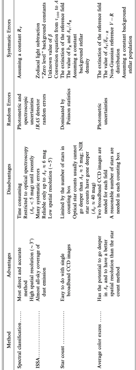
An Extinction Study of the Taurus Dark Cloud Complex

An Extinction Study of the

Taurus Dark Cloud Complex

The Harvard community has made this

article openly available.

Please share

how

this access benefits you. Your story matters

Citation

Arce, Hector G., and Alyssa A. Goodman. 1999. “An Extinction Study

of the Taurus Dark Cloud Complex.” The Astrophysical Journal 517

(1): 264–81. https://doi.org/10.1086/307168.

Citable link

http://nrs.harvard.edu/urn-3:HUL.InstRepos:41397446

Terms of Use

This article was downloaded from Harvard University’s DASH

repository, and is made available under the terms and conditions

applicable to Other Posted Material, as set forth at

http://

THEASTROPHYSICALJOURNAL, 517 : 264È281, 1999 May 20

1999. The American Astronomical Society. All rights reserved. Printed in U.S.A.

(

AN EXTINCTION STUDY OF THE TAURUS DARK CLOUD COMPLEX HECTORG. ARCE1ANDALYSSAA. GOODMAN2

Harvard-Smithsonian Center for Astrophysics, 60 Garden Street, Cambridge, MA 02138 ; harce=cfa.harvard.edu, agoodman=cfa.harvard.edu

Received 1998 May 26 ; accepted 1998 December 29

ABSTRACT

We present a study of the detailed distribution of extinction in a region of the Taurus dark cloud complex. Our study uses new BV R images of the region, spectral classiÐcation data for 95 stars, and

IRAS Sky Survey Atlas (ISSA) 60 and 100 km images. We study the extinction of the region in four di†erent ways, and we present the Ðrst intercomparison of all these methods, which are as follows : (1) using the color excess of background stars for which spectral types are known, (2) using the ISSA 60 and 100 km images, (3) using star counts, and (4) using an optical (V and R) version of the average color excess method used by Lada et al. We Ðnd that all four methods give generally similar resultsÈwith important exceptions. As expected, all the methods show an increase in extinction due to dense dusty regions (i.e., dark clouds and IRAS cores) and a general increase in extinction with increasing decli-nation, due to a larger content of dust in the northern regions of the Taurus dark cloud complex. Some of the discrepancies between the methods are caused by assuming a constant dust temperature for each line of sight in the ISSA extinction maps and not correcting for unexpected changes in the background stellar population (i.e., the presence of a cluster or Galactic gradients in the stellar density and average

V[R color). To study the structure in the dust distribution, we compare the ISSA extinction and the extinction measured for individual stars. From the comparison, we conclude that in the relatively low

-extinction regions studied, with 0.9\A mag (away from Ðlamentary dark clouds and IRAS cores),

V\3.0

there are no Ñuctuations in the dust column density greater than 45% (at the 99.7% conÐdence level), on scales smaller than 0.2 pc. We also report the discovery of a previously unknown open cluster of stars behind the Taurus dark cloud near R.A. 4h19m, decl. 27¡30@(B1950).

Subject headings :dust, extinction È infrared : ISM : continuum È

ISM : individual (Taurus Dark Cloud) È techniques : photometric È techniques : spectroscopic

1.

INTRODUCTION

In order to understand how molecular clouds evolve and eventually produce stars, it is necessary to study the dis-tribution of their star-forming matter. Since the cloudsÏ main constituent, molecular hydrogen, is generally unob-servable, it is necessary to use other tracers, whose abun-dance relative to hydrogen can be reliably estimated, to map out the distribution of material. The extinction of background starlight is the result of the absorption and scattering of photons o† dust grains, so, for a given line of sight, the amount of extinction is directly proportional to the amount of dust. If the gas-to-dust ratio is known and constant (e.g., Bohlin, Savage, & Drake 1978), then a detailed study of the dust distribution in a cloud serves as a detailed study of its mass distribution.

The study of Ñuctuations in the dust distribution is also interesting independent of its usefulness as a mass tracer. Strong Ñuctuations in the dust distribution have consider-able impact on both the physics and chemistry of the inter-stellar medium (ISM), which both depend heavily on the extinction (opacity) structure on all scales (see Thoraval, & Duvert 1997, and references therein). In addition, Boisse,

knowledge of the spatial structure and amount of extinction in the Galactic ISM is important since it a†ects the appar-ent colors of background sources, such as stars and gal-axies.

The most direct measure of reddening is the color excess of a star with known spectral type. Unfortunately, mapping

1National Science Foundation Minority Graduate Fellow.

2National Science Foundation Young Investigator.

out extended distributions of extinction (reddening) by obtaining photometry and a spectrum for large numbers of stars is very tedious and time consuming and usually impractical. Therefore, the traditional way of undertaking an extinction study of a fairly large region of the sky has been, until recently, through the use of optical star counts using photographic plates (Bok & Cordwell 1973). This method can only be used up to an extinction of approx-imately 4 mag, with a resolution [email protected], recent advances in technology have led to the development of new methods of deriving the extinction in dark cloud regions. For example, in a study of the structure of nearby dark clouds, Wood, Myers, & Daugherty (1994) use 60 and 100

km images taken by IRAS to calculate 100 km optical depth, from which they obtain the extinction(A_V).Lada et al. (1994, hereafter LLCB) took advantage of the improve-ments in infrared array cameras to devise a clever new method of measuring extinction. The LLCB technique,3

which combines measurements of near-infrared (HandK) color excess and certain techniques of star counting, has a higher angular resolution and can probe greater optical depths than those achieved by optical star counting alone.

In this study we use four di†erent methods of measuring using (1) the color excess of individual background stars

A

V,

for which we could obtain spectral types, (2) ISSA 60 and 100km images to estimate dust opacity, (3) traditional star counting, and (4) an optical (V andR) version of the average color excess method used by Lada et al. (1994). To our

3This technique has been called the ““ NICE ÏÏ (near-infrared color excess) method by Alves et al. (1998).

TAURUS COMPLEX EXTINCTION STUDY 265

knowledge, this is the Ðrst time that all of these di†erent methods have been directly intercompared. We describe the acquisition and reduction of the data in ° 2. In ° 3 we present the results of the observations, and in°4 we o†er analysis and discussion. Readers interested primarily in intercomparison of the various methods and limits on density Ñuctuations should skim°°2 and 3 and focus more on°°4 and 5. In°5 we compare and rate the four di†erent methods of obtainingA We devote°6 to our conclusions.

V.

2.

DATA

The new photometric and spectroscopic observations used in this paper were originally obtained to conduct the polarization-extinction study described in Arce et al. (1998). The photometry consists ofB,V, andRCCD images of two 10@byD5¡ ““ cuts ÏÏ through the Taurus dark cloud complex (see Fig. 1). In the spectroscopic observations, we observed 95 stars (most of them in cut 1), in order to determine their

FIG. 1.ÈExtinction(A map of part of the Taurus dark cloud region. The map was obtained using the method described in°2.3. The two cuts for which

V)

2000

1500

1000

500

0

Number

22 21 20 19 18 17 16 15 14

mR [mag]

266 ARCE & GOODMAN

spectral types. The cuts shown in Figure 1 pass through two well-known Ðlamentary dark clouds (L1506 and B216[217, both at a distance of 140 pc from the Sun), as well as very low extinction regions, giving our photometric observations a fairly large dynamic range in extinction. In the spectroscopic observations, we selected our target stars along the two cuts by virtue of their relative brightness, in that we attempted to exclude foreground stars by not selec-ting stars that appear unusually bright. Table 1 lists the spectral type, apparentV magnitude andB[V color, and the derived spectroscopic parallax distance for each target star. Our stellar sample has only one star with a distance less than 140 pc, which conÐrms that we largely succeeded in excluding foreground stars. In addition to the new photo-metric and spectroscopic observations we also obtained co-added images of Ñux density from the IRAS Sky Survey Atlas (ISSA), in order to examine the far-infrared emission from dust in the region.

2.1. Photometric Data

The broadband imaging data of the two cuts (Fig. 1) through the Taurus dark cloud complex were obtained using the Smithsonian Astrophysical Observatory (SAO) AndyCam on the Fred Lawrence Whipple Observatory (FLWO) 1.2 m telescope on Mount Hopkins, Arizona. AndyCam is a camera with a thinned backside illuminated AR coated Loral 2048]2048 CCD chip. All the frames were taken in 2]2 bin mode, giving a plate scale of 0A.63 pixel~1. In 1995 November, a total of 64 frames in di†erent positions in the sky were taken in theB,V, andRbands, whereRis the CousinsR-band Ðlter with an e†ective wave-length equal to 0.64km. In each position we obtained one 200 s exposure for each broadband Ðlter. Each telescope pointing was a little less than 10@ north of the previous position, and since each frame is slightly larger than 10@]10@, there is a small sky overlap between the frames successive positions. The Ðrst cut extends from declination of 22¡30@ to 28¡20@, centered on right ascension 4h22m36s

(J2000), with a total of 36 frames. The second cut extends from declination 24¡00@to 28¡30@, centered on right ascen-sion 4h21m29s(J2000), with a total of 28 frames. In addition to the frames acquired in 1995 November, 17 frames were taken in theU,B, andV bands in 1996 October, four frames were taken in theB andV bands in 1996 November, and two frames were taken in the B and V bands in 1997 MarchÈall with the same instrument conÐguration as the 1995 November frames. The additional frames were taken because not all of the original frames were of good quality ; several frames were of regions of special interest around the two dark clouds peripheries (outside the cuts), which the original frames did not include, and because shorter expo-sure images of some of the regions covered by the original frames were needed. The exposure times were 80, 150, and 200 s for V, B, andU, respectively, for frames of new sky positions, and 30 s inV, 50 s inB, and 100 s inUfor frames with repeated positions in the sky.

All of the stellar photometric data reduction was accom-plished using standard Image Reduction and Analysis Facility (IRAF) routines. For stars whose spectra had been measured (see° 2.2), photometry was obtained in the Ñat-Ðelded, background-subtracted images using the APPHOT routine. After analyzing the dependence of magnitude value with aperture size in the standard stars for all nights, it was decided to use an aperture radius of 14 pixels. With this

aperture size, less than 10% of the stars in the most crowded Ðeld, with R-band apparent magnitude (m between 14.5

R)

and 18.0 mag, have neighbors within the aperture. The cor-rection to the standard photometric system was accom-plished using Landolt standards (Landolt 1992). A set of standards were observed for each night, at di†erent times of the night, at varying air masses. These were then used to solve a set of linear equations that would give the starsÏV

magnitude,B[V andV[Rcolors using the routines in the IRAF package PHOTCAL. The errors obtained from the APPHOT routine and the errors in the transformation equation Ðt were summed in quadrature to give the Ðnal errors in the photometry. These were^0.02 to 0.06 mag for

V andB[V for stars withV between 12.3 and 17.4 mag. We calculated the photometry of the standard stars used to derive the transformation equation and compared our results with those quoted by Landolt (1992). By doing so we convinced ourselves that the values of our Ðnal 1p errors (Table 1) are a reasonably good estimation of the true pho-tometry uncertainties.

In addition to obtaining apparent magnitudes and colors for stars, the photometric data were also used to do a star count of the region. The routine DAOFIND was used to detect sources in theRÐlter frames. This routine automati-cally detects objects that are above a certain intensity threshold, and within a limit of sharpness and roundness, all of which the user speciÐes. We used a Ðnding threshold of 5 times the rms sky noise in each frame. The objects detected by the routine are then stored in a Ðle with the objectsÏ coordinates. Although care was taken to select a limit of sharpness and roundness so that DAOFIND would only detect stars, other objects (like cosmic rays and galaxies) were also detected, and some stars clearly above the thresh-old level were not detected. Thus, theRframes were pains-takingly inspected visually to erase detected objects that were not stars and add the few stars that were clearly above the threshold but were not originally detected. We obtained the photometry of all the stars in the sample and then made a histogram (Fig. 2) of the number of stars versus apparent

R magnitude in order to study the completeness of the sample. From Figure 2 we estimate the upper completeness

FIG. 2.ÈHistogram of the distribution of stars with respect to apparent

R-band magnitude(m is shown. These are the stars detected in the 64

R)

R-band frames taken in 1995 November. Stars withm are

saturat-R\14.5

ed in the 200 s exposures, and thus we do not include them in the distribu-tion. From this Ðgure we estimate our sample is at least 90% complete for 14.5¹m

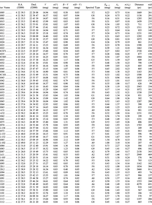
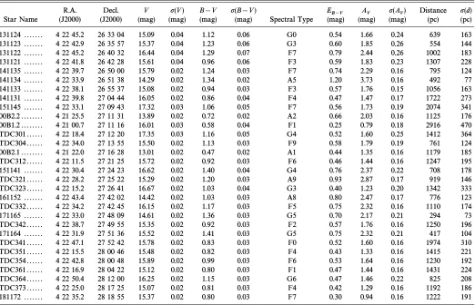
TABLE 1

PHOTOMETRIC ANDSPECTROSCOPICDATA

R.A. Decl. V p(V) B[V p(B[V) E

B~V AV p(AV) Distance p(d)

Star Name (J2000) (J2000) (mag) (mag) (mag) (mag) Spectral Type (mag) (mag) (mag) (pc) (pc)

011005 . . . 4 22 39.3 22 28 08 14.94 0.02 0.58 0.03 F2 0.23 0.73 0.16 1669 261

011003 . . . 4 22 38.5 22 38 47 16.57 0.02 0.97 0.04 G8 0.24 0.75 0.22 1156 291

011001 . . . 4 22 35.5 22 45 39 14.87 0.02 0.62 0.03 F6 0.16 0.51 0.16 1295 202

021015 . . . 4 22 35.5 22 48 02 15.99 0.02 0.83 0.03 F8 0.31 0.97 0.18 1459 235

021014 . . . 4 22 36.2 22 53 01 15.81 0.02 1.07 0.03 G8 0.34 1.05 0.21 711 177

021013 . . . 4 22 36.9 22 57 46 15.41 0.02 0.69 0.06 F6 0.23 0.72 0.23 1511 262

021012 . . . 4 22 39.5 23 03 30 14.94 0.02 0.71 0.03 F7 0.21 0.64 0.16 955 149

021011 . . . 4 22 36.3 23 05 39 15.18 0.02 0.74 0.03 F7 0.24 0.73 0.16 1231 192

00N5.2 . . . 4 22 34.4 23 08 09 14.40 0.02 0.58 0.02 F3 0.21 0.65 0.15 1292 199

031025 . . . 4 22 33.4 23 10 38 15.37 0.02 0.84 0.03 G0 0.26 0.81 0.18 1075 263

031024 . . . 4 22 29.7 23 12 54 15.47 0.02 0.90 0.03 G4 0.26 0.79 0.19 861 212

031023 . . . 4 22 29.7 23 16 11 15.23 0.02 0.69 0.03 F6 0.23 0.70 0.16 1398 219

031022 . . . 4 22 29.9 23 19 32 16.34 0.02 0.94 0.03 F9 0.39 1.21 0.18 1462 236

TDC071 . . . 4 22 22.5 23 20 07 15.60 0.02 0.54 0.03 A9 0.27 0.82 0.17 2720 434

041035 . . . 4 22 33.7 23 28 24 14.57 0.04 0.78 0.07 F7 0.28 0.86 0.25 877 158

TDC085 . . . 4 22 18.6 23 33 10 16.25 0.05 0.81 0.07 F6 0.34 1.07 0.25 1884 342

041033 . . . 4 22 33.6 23 37 38 16.23 0.04 1.17 0.06 G5 0.51 1.59 0.27 809 212

041032 . . . 4 22 32.4 23 41 30 15.01 0.04 0.98 0.06 F7 0.48 1.50 0.23 798 139

041031 . . . 4 22 35.3 23 45 31 16.16 0.04 1.50 0.06 F8 0.99 3.05 0.25 605 109

051045 . . . 4 22 30.2 23 47 47 15.15 0.04 1.07 0.06 F5 0.65 2.02 0.23 805 140

051044 . . . 4 22 34.6 23 52 36 14.90 0.04 0.81 0.06 F3 0.44 1.38 0.23 1163 202

TDC101 . . . 4 22 44.6 23 53 49 15.51 0.04 0.75 0.06 F5 0.33 1.02 0.23 1508 263

051043 . . . 4 22 37.8 23 55 57 16.08 0.02 0.77 0.03 F6 0.31 0.96 0.16 1839 288

051042 . . . 4 22 36.0 23 59 45 15.02 0.02 0.79 0.02 F6 0.33 1.01 0.15 1103 170

051041 . . . 4 22 36.8 24 03 60 14.37 0.02 0.90 0.02 F9 0.35 1.08 0.17 626 99

061055 . . . 4 22 38.7 24 12 10 16.43 0.04 0.84 0.06 F6 0.38 1.19 0.22 1943 334

061054 . . . 4 22 43.4 24 15 44 15.29 0.04 0.87 0.05 F7 0.37 1.14 0.21 1072 181

061053 . . . 4 22 39.6 24 19 04 14.94 0.04 0.74 0.05 F0 0.43 1.32 0.21 1530 259

061052 . . . 4 22 35.9 24 21 58 15.83 0.04 1.03 0.06 G1 0.43 1.34 0.24 951 243

061051 . . . 4 22 37.1 24 24 34 15.09 0.04 1.42 0.05 G9 0.64 1.98 0.26 302 78

071065 . . . 4 22 39.4 24 29 30 16.04 0.04 1.02 0.06 F7 0.52 1.63 0.22 1207 208

071064 . . . 4 22 37.6 24 34 02 12.93 0.02 0.86 0.02 F5 0.44 1.37 0.15 390 60

071063 . . . 4 22 32.9 24 37 16 14.63 0.04 0.95 0.05 F9 0.40 1.25 0.23 655 114

N14.51 . . . 4 22 41.9 24 37 49 14.15 0.02 0.77 0.02 A9 0.50 1.57 0.16 991 155

N14.52 . . . 4 22 58.2 24 40 35 15.25 0.02 0.78 0.03 F6 0.32 1.00 0.16 1231 192

071062 . . . 4 22 40.3 24 41 14 12.82 0.02 1.34 0.02 G9 0.56 1.74 0.30 199 32

071061 . . . 4 22 40.3 24 45 56 15.14 0.04 0.85 0.05 F3 0.48 1.49 0.21 1231 208

081075 . . . 4 22 34.3 24 49 39 15.40 0.04 1.31 0.05 G9 0.53 1.65 0.26 406 105

081074 . . . 4 22 31.2 24 53 44 15.78 0.04 0.93 0.05 F0 0.62 1.93 0.21 1703 288

AG-136 . . . 4 22 44.0 24 57 04 12.32 0.02 0.93 0.02 F7 0.43 1.33 0.15 249 38

081073 . . . 4 22 35.2 24 57 59 15.66 0.04 1.12 0.05 F7 0.62 1.93 0.21 883 149

AG-133 . . . 4 21 48.0 25 05 20 14.15 0.03 0.91 0.04 F7 0.41 1.27 0.18 596 96

AG-132 . . . 4 21 31.0 25 05 48 14.17 0.02 1.14 0.02 G1 0.54 1.67 0.19 379 93

091085 . . . 4 22 30.3 25 09 19 16.96 0.04 2.12 0.09 G0 1.54 4.78 0.33 358 99

AG-102 . . . 4 22 49.0 25 11 23 12.29 0.03 1.27 0.10 A9 1.00 3.10 0.34 207 43

091084 . . . 4 22 31.0 25 12 40 15.91 0.04 1.36 0.06 G3 0.73 2.27 0.24 586 150

091083 . . . 4 22 36.5 25 15 57 16.32 0.04 1.23 0.06 G9 0.45 1.41 0.27 696 182

092087 . . . 4 21 26.0 25 19 49 15.75 0.02 0.85 0.03 A2 0.79 2.45 0.17 2158 343

00Ld.1 . . . 4 21 31.5 25 20 39 15.41 0.02 0.53 0.03 A2 0.47 1.46 0.17 2949 469

AG-105 . . . 4 21 28.0 25 20 51 15.16 0.03 1.29 0.04 G9 0.51 1.58 0.24 376 96

091081 . . . 4 22 34.2 25 25 32 14.22 0.02 0.78 0.02 F5 0.36 1.11 0.15 795 123

101095 . . . 4 22 32.0 25 27 51 15.27 0.02 0.85 0.03 F5 0.43 1.34 0.16 1162 182

0N20.1 . . . 4 22 43.0 25 28 18 16.14 0.03 0.78 0.05 F6 0.32 1.00 0.19 1854 304

0N20.2 . . . 4 22 58.9 25 28 32 16.34 0.03 0.40 0.05 A2 0.34 1.05 0.20 5460 911

101094 . . . 4 22 30.5 25 32 13 13.61 0.02 0.89 0.02 F6 0.43 1.35 0.15 493 76

101092 . . . 4 22 24.3 25 42 15 15.55 0.02 1.01 0.04 F7 0.51 1.57 0.17 986 157

101091 . . . 4 22 30.3 25 44 58 13.27 0.02 0.74 0.02 A8 0.50 1.57 0.16 692 108

0N22.1 . . . 4 22 28.9 25 46 24 14.61 0.02 0.64 0.02 A5 0.50 1.55 0.16 1553 244

111105 . . . 4 22 32.8 25 48 49 16.85 0.02 0.64 0.04 A6 0.48 1.49 0.18 4279 691

111104 . . . 4 22 34.0 25 51 39 14.83 0.02 0.88 0.02 F5 0.46 1.41 0.15 918 142

111102 . . . 4 22 30.2 25 58 31 15.90 0.02 1.24 0.03 G9 0.46 1.43 0.22 567 142

111101 . . . 4 22 38.2 26 02 53 12.76 0.05 1.18 0.10 G1 0.58 1.80 0.35 186 52

121115 . . . 4 22 37.4 26 08 34 14.27 0.04 1.17 0.06 G1 0.57 1.78 0.22 378 97

121113 . . . 4 22 36.1 26 15 12 15.64 0.04 0.93 0.06 F6 0.47 1.45 0.22 1197 206

268 ARCE & GOODMAN Vol. 517

TABLE 1ÈContinued

R.A. Decl. V p(V) B[V p(B[V) E

B~V AV p(AV) Distance p(d)

Star Name (J2000) (J2000) (mag) (mag) (mag) (mag) Spectral Type (mag) (mag) (mag) (pc) (pc)

131124 . . . 4 22 45.2 26 33 04 15.09 0.04 1.12 0.06 G0 0.54 1.66 0.24 639 163

131123 . . . 4 22 42.9 26 35 57 15.37 0.04 1.23 0.06 G3 0.60 1.85 0.26 554 144

131122 . . . 4 22 45.2 26 40 32 16.44 0.04 1.29 0.07 F7 0.79 2.44 0.26 1002 183

131121 . . . 4 22 41.8 26 42 28 15.61 0.04 0.96 0.06 F3 0.59 1.83 0.23 1307 228

141135 . . . 4 22 39.7 26 50 00 15.79 0.02 1.24 0.03 F7 0.74 2.29 0.16 795 124

141134 . . . 4 22 33.9 26 51 38 14.29 0.02 1.34 0.02 A5 1.20 3.73 0.16 492 77

141133 . . . 4 22 38.1 26 55 37 15.08 0.02 0.94 0.03 F3 0.57 1.76 0.15 1056 163

141131 . . . 4 22 39.8 27 04 44 16.05 0.02 0.86 0.04 F4 0.47 1.47 0.17 1722 273

151145 . . . 4 22 33.1 27 09 43 17.32 0.03 1.06 0.05 F7 0.56 1.73 0.19 2074 341

00B2.2 . . . 4 21 25.5 27 11 31 13.89 0.02 0.72 0.02 A2 0.66 2.03 0.16 1125 176

00B1.2 . . . 4 21 00.7 27 11 16 16.01 0.03 0.58 0.04 F1 0.25 0.79 0.18 2916 470

TDC301 . . . 4 22 18.4 27 12 20 17.35 0.03 1.16 0.05 G4 0.52 1.60 0.25 1412 364

TDC304 . . . 4 22 34.0 27 13 55 15.50 0.02 1.13 0.03 F9 0.58 1.79 0.19 761 124

00B2.1 . . . 4 21 22.0 27 16 28 13.01 0.02 0.47 0.02 A1 0.44 1.35 0.16 1179 185

TDC312 . . . 4 22 11.5 27 21 25 15.72 0.02 0.92 0.03 F6 0.46 1.44 0.16 1247 195

151141 . . . 4 22 30.4 27 24 23 16.62 0.02 1.40 0.04 G4 0.76 2.37 0.22 708 178

TDC321 . . . 4 22 28.2 27 25 22 15.29 0.02 1.20 0.03 A9 0.93 2.87 0.17 919 146

TDC323 . . . 4 22 15.2 27 26 41 16.67 0.02 1.03 0.04 G3 0.40 1.23 0.20 1342 333

161152 . . . 4 22 43.4 27 42 02 14.42 0.02 1.03 0.03 A8 0.80 2.47 0.17 776 123

TDC332 . . . 4 22 34.2 27 42 45 16.15 0.02 1.17 0.03 F5 0.75 2.32 0.16 1110 174

171165 . . . 4 22 33.0 27 48 09 14.61 0.02 1.36 0.03 G5 0.70 2.17 0.21 294 73

TDC342 . . . 4 22 38.7 27 49 55 15.35 0.02 0.92 0.03 F2 0.57 1.76 0.16 1250 196

171164 . . . 4 22 31.9 27 51 36 15.52 0.02 1.41 0.03 G5 0.75 2.32 0.21 417 104

TDC341 . . . 4 22 47.1 27 52 42 15.78 0.02 0.83 0.03 F0 0.52 1.60 0.16 1974 310

TDC351 . . . 4 22 15.5 28 00 46 15.48 0.02 0.82 0.03 F4 0.43 1.33 0.16 1415 221

TDC354 . . . 4 22 42.8 28 00 48 15.89 0.02 0.99 0.03 F6 0.53 1.64 0.16 1230 192

TDC361 . . . 4 22 16.9 28 04 22 15.12 0.02 0.80 0.03 F1 0.47 1.44 0.16 1431 224

TDC364 . . . 4 22 50.4 28 12 00 16.25 0.02 1.15 0.03 G6 0.47 1.46 0.22 825 208

TDC373 . . . 4 22 25.0 28 17 25 15.07 0.02 0.81 0.03 F4 0.42 1.29 0.16 1192 186

181172 . . . 4 22 35.2 28 18 55 15.37 0.02 0.80 0.03 F7 0.30 0.94 0.16 1222 191

NOTE.ÈUnits of right ascension are hours, minutes, and seconds, and units of declination are degrees, arcminutes, and arcseconds.

limit to bem_RB18.0mag. Stars brighter than 14.5 mag in theR-band 200 s exposures are saturated ; thus, the photo-metry of stars with m_R\14.5 is unreliable. Therefore we estimate that our sample is at least 90% complete for stars with 14.5¹m

R\18.0.

2.2. Spectroscopic Data

The spectra of 95 stars along the cuts were obtained using the SAO FAST spectrograph on the FLWO 1.5 m telescope on Mount Hopkins, Arizona. The observations were carried out during the fall trimesters of 1995 and 1996. FAST was used with a 3A slit and a 300 line mm~1 grating. This resulted in a resolution of D6 AŽ , a spectral coverage of

D3800 AŽ (from approximately 3600 to around 7400 AŽ), a dispersion of 1.47 AŽ pixel~1, and 1.64 pixels arcsec~1

along the dispersion axis.

The spectrum of each star was used to derive its spectral type. In order to spectroscopically classify the stars, we fol-lowed OÏConnell (1973) and Kenyon, Dobrzycka, & Hartman (1994) and computed several absorption-line indices from the spectra :

I

j\ [2.5 log

C

F(j₂)

F@(j₂)

D

where

F@(j₂)\F(j₁)][F(j₃)[F(j₁)]

C

j 3[j1

D

is the interpolated continuum Ñux at the feature,j₁andj₃

are continuum wavelengths, j is the feature wavelength,

2

andF(j_i)is the average Ñux in ergs cm~2s~1AŽ ~1 over a bandwidth speciÐed in Table 2 of OÏConnell (1973). We measured the CaIIH (j3933), Hd(j4101), CH (j4305), Hv

No. 1, 1999 TAURUS COMPLEX EXTINCTION STUDY 269

Once each star was classiÐed, its reddening was calcu-lated. Intrinsic B[V values for each spectral type were obtained from Table A5 in Kenyon & Hartmann (1995). The observedB[V value, from the photometric study, was then used to obtain the color excess :E_B~V\(B[V)[(B

where (B[V) is the observed color index and

[V)

0,_{is the unreddened intrinsic color of the star. An error}(B [V)₀

in the stellar classiÐcation of^1È2 subclasses in AÈF stars transforms into an error of ^0.04È0.05 mag in E

B~V,

whereas an error in the stellar classiÐcation of^2È4 sub-classes in G stars transforms into an error of ^0.05È0.08 mag inE_B~V.We assumed thatA_V\R_VE_B~V,withR_V(the ratio of total-to-selective extinction) equal to 3.1 (Savage & Mathis 1979 ; Vrba & Rydgren 1985)Èthe validity of this assumption is discussed below. Using absolute magnitude values for each spectral type from Lang (1992), we then obtained distances for each star (see Table 1).

When we calculated the extinction to each star using a constant value ofR_V\3.1, we made the implicit assump-tion that the ratio of total-to-selective extincassump-tion is constant for di†erent lines of sight. In fact,R_Vvaries along di†erent lines of sight in the Galaxy and only has a mean ofD3.1 (Savage & Mathis 1979). In contrast with other regions, the Taurus-Auriga molecular cloud complex seems to have a fairly constant interstellar reddening law with R

VB3.1

through most of the region (Vrba & Rydgren 1985 ; Kenyon et al. 1994). OurBV Rphotometry is not ample enough to derive R_V for each line of sight. We would need obser-vations at shorter wavelengths to be able to independently obtain the value of the ratio of total-to-selective extinction for each line of sight we observed. Thus we decided to use the ISM (and Taurus) average ofR and to caution

V\3.1

the reader that we do not take the errors caused by assuming a constantR into account when we calculate the

V

errors inA_V. In°3.1 we show how the ISSA data conÐrm that R is a good estimate of the ratio of

total-to-V\3.1

selective extinction for our region.

2.3. ISSA Data

TheIRAS Sky Survey Atlas (ISSA) was used to obtain images of Ñux density at 60 and 100km of the Taurus dark cloud complex. Our region of interest lies in two di†erent (but overlapping) ISSA Ðelds. Each of these is a 500]500 pixel image, covering a12¡.5by12¡.5Ðeld of sky with a pixel size [email protected] maps have units of MJy Sr~1, are made with gnomic projection, have spatial resolution smoothed to the

IRASbeam at 100km (approximately 5@), and the zodiacal emission has been removed from them. The12¡.5 by12¡.5

images were cropped in order to keep only the region of the Taurus dark cloud complex shown in Figure 1. This resulted in a total of four di†erent images : two (60 and 100

km) images of the northern part and two images of the southern part of the map.

Although they have the zodiacal emission removed, ISSA Ðelds are not calibrated so that the ““ zero point ÏÏ corre-sponds to no emission, so another ““ background ÏÏ needs to be subtracted. This background-subtraction procedure went as follows. First, the minimum value of each of the four 12¡.5 by 12¡.5 images (see Table 2) was obtained and subtracted from them. The resulting images were then used to obtain an optical extinction(A map through a process

V)

to be discussed below. At this point, after just a simple subtraction of the minimum value in each image, the north and the southA_Vmaps (see Fig. 1) did not agree within the errors in the region of overlap. So, the values used for the background subtraction were iterated until the best agree-ment for the overlap region was found while keeping the background-subtraction constants less than 1 MJy Sr~1

away from the minimum Ñux value of the original12¡.5 by ISSA Ðelds. Table 2 lists the values that were ultima-12¡.5

tely used for this purpose. These values resulted in a di†er-ence of 0.1 mag between the mean in the distribution ofA_V

values in the northern image and the mean in the distribu-tion ofA_Vvalues in the southern image. Tests using other values for background subtraction showed that the result-ant extinction values did not change signiÐcresult-antly for small (less than D1 MJy Sr~1) changes in the background-subtraction constants. As discussed below, the o†set between ISSA plates winds up being the limiting error in determining extinction from ISSA data.

The extinction map was computed from the ISSA images using a method very similar to that described by Wood et al. (1994), and references therein. Note, however, that in their study, Wood et al. (1994) usedIRASimages that had not gone through a zodiacal emission removal process. They devised their own zodiacal light subtraction, which they state is not very efficient for regions near the ecliptic, like Taurus. One of the regions they study was in fact the Taurus dark cloud region itself. We believe that our extinc-tion map is of better quality because we use ISSA images that have a more elaborate zodiacal light subtraction algo-rithm.

The 60 and 100km dust temperatureT_dat each pixel in an image can be obtained by assuming that the dust in a single beam can be characterized by one temperature (T_d), and that the observed ratio of 60 to 100km emission is due to blackbody radiation from dust grains atT_d,modiÐed by

TABLE 2

BACKGROUNDSUBTRACTION FORISSA IMAGES

MINIMUMFLUX BACKGROUND-SUBTRACTIONCONSTANT

100km 60km 100km Flux 60km Flux

IMAGE (MJy Sr~1) (MJy Sr~1) (MJy Sr~1) (MJy Sr~1)

Northa. . . 8.89 [0.57 8.50 [0.70

Southb. . . 7.27 [1.05 6.60 [1.04

aThe north images come from the ISSA images i311b3h0 and i311b4h0, which are cen-tered at 4h36m, 30¡ (B1950).

270 ARCE & GOODMAN Vol. 517

a power-law emissivity. The Ñux density of emission at a wavelengthj_i,is given by

F_i\

A

i

3

1

ehc@jikTd[1

B

daji~b)i, (3)

where N_d is the column density of dust grains, b is the power-law index of the dust emissivity,) is the solid angle

i

atj_i,andais a constant of proportionality.

In order to use equation (3) to calculate the dust color temperature(T_d)of each pixel in the image, we have to make some assumptions. The Ðrst assumption is that the dust emission is optically thin. We believe this is a safe assump-tion because in our maps there is not a single line of sight that could be optically thick(q In fact, the largest

100[1).

we Ðnd in our processed images is 0.002. The second

q₁₀₀

assumption we have to make is that) which is

60+)100,

true for all ISSA images. With these two assumptions we can then write the ratioRof the Ñux densities at 60 and 100

km as

R\ F60 F

100

\0.6~(3`b)

A

B

In order to proceed we need to assume a value of b. For now we will assume that b\1, and we will discuss the implications of this assumption later on. We constructed a look-up table with the value of R calculated for a wide range ofT_d,with steps inT_dof 0.05 K. For each pixel in the image, the table was searched for the value ofT that

repro-d

duces the observed 100 to 60km Ñux ratio. Using the dust color temperature, we then calculate the dust optical depth for each pixel

q₁₀₀\Fj(100km)

B

j(j,Td)

, (5)

whereB_j(j,T_d)is the Planck function andF_j(100km) is the observed 100km Ñux.

We use equation (5) of Wood et al. (1994) to convert from optical depth to extinction inV:

A_V\15.078(1[e~q100@a) , (6) whereq is the optical depth and a is a constant with a

100

value of 6.413]10~4. This equation relies on the work of Jarrett, Dickman, & Herbst (1989), who present a plot (their Fig. 8) of the relation between 60km optical depth(q₆₀)and based on star counts. Assuming optically thin emission,

A_V

Wood et al. (1994) multiply the Jarrett et al. (1989) q 60

values by 100/60 to convert toq₁₀₀and obtain equation (6), above. Thus, extinction values obtained using the ISSA images are subject to the uncertainties in the conversion equation. But, Figure 8 of Jarrett et al. (1989) shows that there is a very tight correlation between q₆₀ and A_V for mag, implying very little uncertainty in the

conver-A_V¹5

sion of far-infrared optical depth to visual extinction. In the Taurus region under study in this paper, all of the extinc-tion values measured are less than 5 mag, so we do not consider any errors caused by uncertainty in the coefficients of equation (6).

After all this processing was done, we were left with two extinction maps (a northern and a southern one) that had some overlap (see Fig. 1). The area of overlap was averaged and the north and south extinction maps were combined to produce a Ðnal image (Fig. 1) extending from R.A. of

4h09m00sto 4h24m30s(B1950) and from decl. 22¡00@to 28¡35@

(B1950).

An interesting point to note is that several ““ elliptical holes ÏÏ in the extinction appear in Figure 1. These ““ holes ÏÏ are unphysical depressions in the extinction produced by the hot sources seen in the 60km maps. The 60km point sources (mostly embedded young stars) heat the dust around them and create a region where there is an excess of hot dust. This limitation, caused by the low spatial resolution of IRAS and assuming a single T_d, will then create an unphysically low extinction, when calculating the in the region nearIRASpoint sources, using the method

A_V

described above. Unfortunately, cut 2 (see Fig. 1) passes near two of these unphysically low-extinction areas. (In Figs. 4 and 6 we mark the position of the unreal dip in extinction.) These unphysical holes inA are each

associ-V

ated with two very close IRAS point sources (one hole is produced by IRAS 0418]2654 and IRAS 0418]2655 and the other one by IRAS 0418]2650 and IRAS 0419]2650) inside the dark cloud B216[217 (see end of°3.2).

As mentioned above, in order to calculate the optical depth we assumed that the dust emissivity is proportional to a power law (q_dPj~b), with index b\1. Although studies di†er in the values they Ðnd forb, there is a general agreement that the emissivity index depends on the grainÏs size, composition, and physical structure (Weintraub, Sandell, & Duncan 1991). The general consensus in recent years has been thatbhas a value most likely between 1 and 2, that in the general ISM b is close to 2, and in denser regions with bigger grains b is closer to 1 (Beckwith & Sargent 1991 ; Mannings & Emerson 1994 ; Pollack et al. 1994). Our region of interest has both lines of sight that pass through low- and high-density medium with di†erent environments. Thus, there is no way we can use a ““ perfect ÏÏ or ““ preferred ÏÏ value of b, since it might be di†erent for di†erent lines of sight. In our case we had to choose the same value as Jarrett et al. (1989) and Wood et al. (1994), which is b\1, since we use their results to convert from to extinction. The errors introduced by assuming a

q₁₀₀

constant bare hard to estimate, since we do not have any way to measure how muchbchanges in our region of study. We do not include these errors in the error estimate ofA_V

using ISSA images (from now onA but it must be kept

VISSA),

in mind thatbis not necessarily equal to 1 and that its value may vary for di†erent lines of sight.

In order to estimate the pixel-to-pixel (random) errors in we examined a circular area of 800 pixels centered at

A_V

ISSA,

4h19m, 22¡24@ (B1950), which appears to have a constant extinction. We compared pixels that are 1.5 IRAS beams apart and obtained a standard deviation in the extinction value of this region to be 0.06 mag. We use this value as an estimate of the pixel-to-pixel errors inA

VISSA.

Ultimately, though, we need an estimate of the total error inA_V not just pixel-to-pixel errors. As explained above,

ISSA,

the north and south extinction maps give slightly di†erent extinction values for matching pixels in the region where they overlap. By Ðtting a Gaussian to a histogram of the di†erence inA_V value between the north and the south

ISSA

extinction map, we Ðnd a 1pwidth of 0.11 mag. We use this value as an estimate of the 1 p error in A_V caused by

ISSA

uncertainty in the zero level constants and zodiacal subtrac-tion in the ISSA plates. Adding this ““ plate-to-plate ÏÏ error in quadrature to the pixel-to-pixel error (previous paragraph) gives a total error inA of 0.12 mag. We use

No. 1, 1999 TAURUS COMPLEX EXTINCTION STUDY 271

this value as an estimate of the error in A_V but we

ISSA,

remind the reader that this error does not include any errors caused by assuming a constantb.

3.

RESULTS

The data described above o†er the opportunity to measureA_Vin four di†erent ways : (1) using the 85 stars in cut 1 for which we have color excess data (see Table 1), (2) using 60 and 100km ISSA images as described in°2.3, (3) using star-counting techniques on theR-band frames, and (4) using an optical (V andR) version of the average color excess method used by LLCB, described in more detail in

°3.3.

Throughout the paper we assume that the extinction we calculate, independent of the way it was obtained, is pro-duced by the dust associated with the Taurus dark cloud complex at a distance of 140^10 pc (Kenyon et al. 1994). The region of Taurus we observed lies at Galactic coordi-natelB172¡,bB[17¡. Thus, our stars lie toward lines of sight where there is little or no dust except for that associ-ated with the Taurus dark cloud, and we can safely assume that in the area under study, virtually all the extinction is produced by the dust associated with the Taurus dark cloud complex.

3.1. Extinction from the Color Excess of Stars with Measured Spectral T ypes

Using the color excess and position data for the stars in Table 1 that lie on cut 1 and have a distance larger than 150 pc, we construct the extinction versus declination plot shown in Figure 3a. This technique easily detects the rises in extinction associated with Tau M1 around decl. 23¡.65, L1506 around decl. 25¡, B216[217 around 26¡.7, and the area near theIRAS cores Tau B5 and Tau B11 (hereafter Tau B5ÈB11) around decl. 27¡.5. As in the ISSA A_V map (Fig. 1), the extinction obtained from the color excess of stars(A shows an overall rise in extinction with

increas-Vsp)

ing declination. Also plotted in Figure 3aare the extinction values obtained from the ISSA extinction map(A for

VISSA)

the same coordinates on the sky where there is an A_V

sp

point. The value of eachA point is obtained from the

VISSA

pixel nearest to the coordinates of each star with measured in cut 1. The error bars, set at ^0.12 mag for each

A_V

sp _{point, show the total error (including pixel-to-pixel}

A_V

ISSA

and plate-to-plate variations, but not including systematic errors) discussed above.

As a check on the assumed value ofR_V, we letR_V vary in the calculation of A and then calculate

Vsp *tot\

(whereirepresents theith point in

£

i/1

N oR_VE_B~V[A_V

ISSAoi

the plot) for di†erent values ofR We found that

V. RVD3.05

minimizes the di†erence between the two curves(*_tot).This reassures us that the choice of a constantR_V\3.1is a good assumption.

The traces ofA_V versus declination in Figure 3a show a very striking similarity. Although the beam size of ISSA is

D5@andA_V has a beam, due to seeing e†ects, of

approx-sp

imately 3A (which transform into 0.2 and 0.002 pc, respec-tively, at a distance of 140 pc), both values agree within the errors in most places. A plot of(A_V versus

decli-sp[AVISSA)

nation is shown in Figure 3b. It can be seen that A

Vsp

within errors, for all points not in the vicinity

[A_V

ISSAB0,

of a steep increase in extinction (i.e., away from dark clouds

and IRAS cores). In other words, in the low-extinction regionsA is very similar to despite the great

di†er-Vsp AVISSA,

ence in the resolution of the two methods. This leads us to believe that there are no or only very small Ñuctuations in the extinction inside a 5@beam, inlow-A_Vregions. In order to put an upper limit to the magnitude of the Ñuctuations,

we present a plot of A_V divided by in

sp[AVISSA AVISSA,

Figure 3c. We discuss this plot more in°4.1.

The gently sloping solid lines in Figures 3b and 3c are unweighted linear Ðts to the points in each of the plots. Both Ðts have a very small, but detectable, slope (0.1 mag deg~1

for Fig. 3b). Previous studies usingIRASdata have attrib-uted the existence of gradients like these to imperfect zodia-cal light subtraction (Wood et al. 1994). Moreover, the fact that the linear Ðt of the middle panel crosses the A_V

sp

zero line at a declination of around near the

[A_V

ISSA 25¡.4,

middle of the overlap region between the northern and southern A (Fig. 1) map, leads us to believe that the

VISSA

small gradient is due to imperfect ISSA image reduction. The gradient inA gives a pixel-to-pixel o†set of 0.008

VISSA

mag beam~1, which is much less than the pixel-to-pixel random errors in A and much, much less than other

VISSA

systematic errors (e.g., constant b) so we do not need to correct for it.

3.2. Star Counting

With the help of IRAF, as described in°2.1, we located a total of 3715 stars in cut 1 and 3074 stars in cut 2, with from the 1995 NovemberR-band images. 14.5¹m

R\18.0,

With this database of stellar positions we measure the extinction over the region covered by both cuts, using clas-sical star-counting techniques. First, we subdivide each cut into a rectilinear grid of overlapping squares, and then we count the total number of stars in each square. Our ultimate goal in star counting is to obtain the extinction of the region in a way that can be compared to the other techniques used in this paper. Therefore, in order to mimic the resolution and sampling frequency of the ISSA data, we made the counting squares 5@on a side (the resolution of ISSA) and the centers of the squares were separated [email protected](the size of an ISSA pixel).

Conventionally, measuring extinction from star counts involves comparing the integrated number of stars within a given cell toward the region of interest to a nearby reference Ðeld that is assumed to be free from extinction (Bok & Cordwell 1973). Several assumptions need to be made in order to use this method : (1) the population of stars that are background to the region of interest does not vary substan-tially and is similar to the reference Ðeld, (2) the extinction (A) is uniform over the count cell, and (3) the integrated surface density of stars for the reference Ðeld(N_ref) of stars brighter than the apparent magnitude,m, follows an expo-nential law withlog [N_ref(\m)]\a]bm. The integrated surface density of stars for any other Ðeld under study,N_on, follows a similar law, log [N

on(\m)]\a]b(m[A).

In our case, the extinction to each square was obtained via

A

Von\AVref]

A_V A_R

log (n_ref/n_on)

b_R , (7)

whereA is the extinction of the reference Ðeld, is the

Vref nref

number of stars in the reference Ðeld, andn_onis the number of stars in any of the other counting cells. The quantityb is

5

4

3

2

1

0

Av

[mags]

28 27

26 25

24 23

Declination [deg] (B1950)

Tau M1

L1506

B216-217

Tau B5-B11

reference field in section 3.3 Extinction from spectra

Extinction from ISSA

a

1.5

1.0

0.5

0.0

-0.5 -1.0

AV

sp

-A

VISSA

[mag]

28 27

26 25

24 23

Declination [deg] (1950)

b

2.5

2.0

1.5

1.0

0.5

0.0

-0.5

(A

Vsp

- A

VISSA

)/A

VISSA

28 27

26 25

24 23

Declination [deg] (B1950)

c

FIG. 3.È(a) Shows the extinction of every star we classiÐed by spectral type with distances larger then 140 pc in cut 1, as well as the extinction at the same position on the sky using the ISSA extinction map (Fig. 1). The error bars shown represent only the 1prandom errors for each of the two methods. Also shown in (a) is the region used as reference Ðeld for the extinction obtained using the technique described in°3.3. (b) Shows the di†erence between the two di†erent extinction values from (a). (c) Shows the di†erence (from [b]) divided by the ISSA extinction(A The solid lines in (b) and (c) are the unweighted

VISSA).

linear Ðts to the points in each of the two plots. These lines indicate the small gradient in extinction with declination inA which we believe is due to an

TAURUS COMPLEX EXTINCTION STUDY 273

the slope of the cumulative number of stars as a function of

R apparent magnitude (see assumption [3] in previous paragraph). We calculateb_Rby Ðtting a line tolog [N_ref(\

for and obtain a value of 0.34^0.02.

m

R)] 14.5¹mR\18.0

The ratio A_V/A_R is the reddening law between V and R

wavelengths, which gives the value of 1.24 (He et al. 1995) used in the conversion for star counts in (Cousins) R to extinction inV.

As mentioned above, in conventional star count studies, the reference Ðelds are areas in the sky, close to the region under study, which haveA This is not so in our case.

Vref\0.

Since our CCD data were not originally obtained for star-counting purposes, we did not take any images of a refer-ence Ðeld with A_V Thus, the reference Ðelds were

ref\0.

chosen to be regions where we could safely assume the value of A_V SpeciÐcally, the reference Ðelds were chosen by

ref.

virtue of their having a spectroscopic probe star to which we derived the extinction through its color excess.

One of the major assumptions in conventional star-counting studies is that the population of background stars to the cloud is similar to that in the reference Ðeld. This is why star count studies are only done over small regions of the sky. In our case, cut 1 (the longer cut) expands 6¡ in declination that transforms to nearly 4¡ in Galactic latitude This span in Galactic latitude is ([18¡.8\b\[14¡.9).

enough to have a big e†ect on the surface density of stars due to Galactic variations ; one detects more stars per cell, for a constantA_V,the closer one observes to the Galactic plane. (The star count Galaxy model of Reid et al. 1996 predicts that a 10 deg2Ðeld with no extinction centered at

b\ [14¡,l\ [172¡ will have approximately a factor of 2 more stars than a 10 deg2Ðeld with no extinction centered at b\ [19¡, l\ [172¡.) Thus, it was imperative that we correct for Galactic changes in the stellar density. Not doing this would have resulted in an unreal drop in the derived extinction for lower Galactic latitudes. We account for the Galactic gradient by using four di†erent, more or less evenly spaced, reference Ðelds at di†erent Galactic lati-tudes along the cut. Each of these Ðelds has a star with measured reddening (from Table 1), which was used to esti-mate the extinction of the reference Ðeld in question. Thus, for example, the star count extinction located betweenb\

and (which transforms to

[18¡.9 b\ [17¡.9 22¡25@¹

in cut 1) is tied to the reference Ðeld where

d_J2000\23¡56@

star 011001 lies, the star count extinction in the region with (which transforms to

[17¡.9¹b\[16¡.9 23¡56@¹

in cut 1) is tied to the reference Ðeld where

d_J2000\25¡25@

star 051043 lies, and so forth. The number of stars(n the

ref),

visual extinction(A_V and the range inbII, which each of

ref),

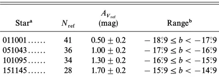
the four reference Ðelds calibrates are given in Table 3. It is important to stress that by doing this calibration we are

TABLE 3

CONTROLFIELDS FORSTARCOUNT

A

Vref

Stara N

ref (mag) Rangeb

011001 . . . 41 0.50^0.2 [18¡.9¹b\[17¡.9 051043 . . . 36 1.00^0.2 [17¡.9¹b\[16¡.9 101095 . . . 34 1.30^0.2 [16¡.9¹b\[15¡.9 151145 . . . 28 1.70^0.2 [15¡.9¹b\[14¡.9

aEach reference Ðeld is tied to only one spectroscopic star.

bThe star count extinction in the given range ofbIIis cali-brated using the reference Ðeld of the respective star.

tyingA_V to at these four points, and thus is not

sc AVsp AVsc

totally independent ofA But this procedure only forces

Vsp.

to agree in absolute value to in four points and not

A_V

sc AVsp

to give the same structure or scale through the cuts.

In our study, where observations lie primarily along a declination cut, the best way to graphically compare the extinction measured by star counting (A_V and from the

sc)

ISSA images(A_V is to plot them both in an extinction

ISSA)

versus declination plot. (Cut 1 is about 6¡ long, but only 10@

wide, giving a ratio of 1 : 36 between length and width. This makes it practically impossible to show a legible Ðgure of a star count extinction map of the cuts.) A value of the extinc-tion was obtained for each 5@]5@ counting box and then averaged extinction over right ascension for every point in declination, so as to produce only one value ofA_Vfor each declination, independent of right ascension. Constant decli-nation slices every 5@ show that the variations in A_V

ISSA

across the 10@ width of each cut are not large. Most of the constant declination slices had standard deviations inA_V

ISSA

of less than 0.2 mag, and none exceeded 0.3 mag. Moreover, most adjacent counting boxes with the same declination di†er inA by less than 0.2 mag. Therefore, we are

con-Vsc

Ðdent that we are not introducing large errors by averaging the extinction over theD10@spanned by each cut in right ascension. On the other hand, by averaging over right ascension, the sensitivity to small-scale Ñuctuations decreases. The smoothed (averaged) extinction trace has less sensitivity in detecting Ñuctuations on 5@scales than on 10@

scales, where it reaches full sensitivity. Nevertheless, averag-ing the extinction over right ascension does not create any disadvantage for the purpose of comparing the di†erent ways of calculating the extinction since all the techniques are averaged over the same width.

Figure 4 showsA and (now both averaged over

Vsc AVISSA

theD10@ that spanned each cut in right ascension) versus declination for both cuts.4 The random errors in the star count trace are plotted for each point. The uncertainty in the number of stars in each sampling box is given by n1@2

(Poisson statistics), wheren is the number of stars counted in the box (Bok 1937). The uncertainty in the extinction (with contributions from the uncertainty inn,n and

ref,AVref,

for each sampling box with the same declination is then

b_R)

averaged to give the Ðnal (plotted) error in the extinction. Like the ratio of total-to-selective extinction(R_V),the value ofA_V/A_Rmay vary from one line of sight to the other. Also, like R_V in ° 2.2, here we use the ISM average value of We do not take the errors caused by assuming a

A_V/A_R.

constant value ofA into account when we calculate the

V/AR

errors inA_V as we have no way of calculating them.

sc,

It can be seen that bothA and show the same

VISSA AVsc

gross extinction structure. Both have local maxima and minima in the same places (in most cases), but not at neces-sarily the same value. Both traces detect rises in extinction associated with Tau M1, L1506, B216[217, and Tau B5ÈB11. It is clear thatA has more Ñuctuations than the

Vsc

trace. These Ñuctuations are not likely to be real, as

A_V

ISSA

most of them are of the same magnitude as the errors in Most of the ““ noise ÏÏ in the extinction resulted because

A_V

sc.

the star count technique is very dependent on the

assump-4Notice thatA in Fig. 4 is an average over the approximately 10@

VISSA

width of the frames taken in the optical, but still has resolutionD5@along the declination direction. Thus, these are not exactly the same values of shown in Fig. 3, where values for single ISSA pixels, with 5@

A

VISSA AVISSA [email protected]

6

5

4

3

2

1

0

AV

[mag]

28 27

26 25

24 23

Declination [deg] (1950)

Tau M1

L1506

B216-217

Tau B5-B11

A_V using ISSA

A_V using star counts

Cut 1

6

5

4

3

2

1

0

AV

[mag]

28 27

26 25

24 23

Declination [deg] (B1950)

L1506

B216-217

Tau B5-B11

Unphysical dip in A_VISSA

Cut 2

274 ARCE & GOODMAN Vol. 517

FIG. 4.ÈPlots of extinction vs. declination for both cut 1 and cut 2. The solid line is the extinction obtained through star counts. The dotted line is the extinction obtained using the ISSA 60 and 100km images. Both methods are averaged over the 10@width of the cut. Breaks in the star count extinction trace are due to missingR-band frames. The error bars in the star count extinction represent the 1perror. The rise in extinction associated with the dark clouds andIRAScores is identiÐed. The dip in the extinction peak associated with B216[217 in theA trace of cut 2 is due to an unreal drop in the extinction

VISSA caused by the presence ofIRASpoint source in the images.

tion of a constant background stellar surface density. Real (small) changes in the background surface density of stars (not caused by extinction) will produce unreal Ñuctuations in the resultantA

Vsc.

Note the unreal dip in the cut 2 trace ofA_V (see Fig. 4),

ISSA

caused by assuming a constant dust temperature for those

lines of sight where there areIRASpoint sources that heat the dust around them (see°2.3). This shows the potentially large errors inA_V that can arise from assuming a single

ISSA

dust temperature(T for each line of sight. The other place

d)

where there is a signiÐcant discrepancy betweenA_V and

ISSA

is in the rise in extinction associated with Tau B5ÈB11

A

60

50

40

30

20

10

0

Number

1.4 1.2 1.0 0.8 0.6 0.4 0.2 0.0 -0.2

V-R [mag]

No. 1, 1999 TAURUS COMPLEX EXTINCTION STUDY 275

(see Fig. 4), where the two methods disagree by more than 1pof the error in A This discrepancy will be discussed

Vsc.

further in°4.2.

3.3. Extinction Measured via Average Color Excess Method

Taking advantage of the fact that we had taken our 1995 November images in more than one broadband Ðlter, we used the method developed by LLCB to study the extinc-tion along both cuts in yet another way. This method con-sists of assuming that the color distribution of stars observed all along the cut is identical in nature to that of stars in a control Ðeld. With this assumption one can use the meanV[Rcolor of the stars in the control Ðeld to approx-imate the intrinsic V[R color of all stars that are back-ground to the cloud. (Note that LLCBÏs analysis was in the near-infrared, and they used H[K colorsÈwhich have even less intrinsic variation thanV[Rcolors.) If we use the same technique as in star counting, the region under study is divided into a grid of overlapping counting boxes, and then an average of the color excess (and extinction) of the stars in each counting box is obtained.

To derive extinction from the average color excess method, we used the same sample of stars, with 14.5¹

used in our star-counting study (° 3.2). The

m

R\18.0,

region between declinations 22¡.9 and 23¡.22 (B1950) was used as our reference Ðeld since, as can be seen in Figure 3a, this region has a uniform extinction within the errors. We took an average of the extinction of the six stars for which we had spectral types and which lie inside this region, and obtained a value of A_V We did not divide

ref\0.72^0.2.

the area under study into square sampling boxes as is usually done in star count studies (see previous section). Instead, the area under study was divided into rectangular cells, where the right ascension side of the rectangle was dictated by the framesÏ width (D10@) and the declination side was set to be 5@. The centers of the rectangles were separated in declination [email protected]. This was done in order to keep the same resolution and sampling frequency in the declination direction as in the ISSA and star-counting methods (described in the previous sections). We are not sensitive to any variations in extinction within each mea-surement rectangle, but Figure 3asuggests that such varia-tions are very small.

The number of stars in each rectangle was counted and the color excess of each star was obtained using the formula :

E

V~R\(V [R)[SV [RTref, (8)

whereSV[RT_ref is the mean V[Rcolor of the reference Ðeld, which in our case is 0.60^0.05 mag. Figure 5 shows the distribution ofV[Rcolors in the reference Ðeld.5We then apply equation (8) to each star in a counting rectangle and obtain a mean color excess to each rectangle :

SE_V~RT\;iN(EV~R)i

N , (9)

whereNis the number of stars in a counting rectangle and is the color excess of theith star. The mean visual (E

V~R)i

5Notice that the width of the color distribution in Fig. 5 is signiÐcantly larger than the error in the mean (0.05 mag). The spread in near-IR (e.g.,

H[K) color for a Ðeld like this would be much narrower, which is why it is preferred to use the average color excess method in the near-IR (LLCB).

FIG. 5.ÈDistribution of V[R colors in the reference Ðeld for the average color excess method described in°3.3.

extinction is obtained using

SA_VT\A_V

ref]

A

V

E

V~R

]SE_V~RT , (10)

whereA_V is the extinction of the reference Ðeld (0.72 mag),

ref

and we use the ISM average value of 5.08 for the expression (He et al. 1995). Similar to the extinction from star

A_V/E_V~R

counts, the extinction using the average color excess (from now onA is not totally independent of the spectral

clas-Vce)

siÐcation method. Recall thatA_V which is used to

cali-ref,

brateA is determined using measurements of This

Vce, AVsp.

calibration forces A_V to agree in absolute value with the

ce

average ofA in the reference Ðeld, but it does not force

Vsp

to give the same structure or scale in the extinction

A_V

ce

curves throughout the cuts.

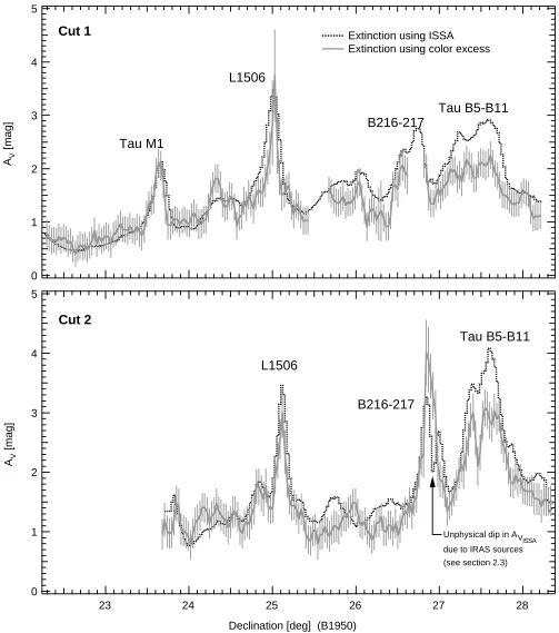
Using the average color excess technique, we are able to detect the same overall trends in extinction found from the ISSA plates, spectral analysis, and star counting (see Fig. 6). The rises in extinction due to Tau M1, L1506, B216[217, and Tau B5ÈB11 can be seen as well-pronounced peaks in

Again, note the unreal dip in the cut 2 trace of

A_V. A_V

ISSA,

caused by the presence of four IRAS point sources in the dark cloud B216[217 (see°2.3). In Figure 6 we also show the random errors of each point in theA_V trace. The

mea-ce

surement uncertainty inA for any given counting cell is

Vce

given by

p_AV

ce\

S

ref

2 ](5.08)2

A

1

N p_(V~R)

i

2

N2

B

wherep_refis the uncertainty inA_V (which is equal to 0.2

ref

mag), N is the number of stars in the counting cell, and is the photometric error in V[R of the ith star

p_(V~R)

i

inside the cell. The quantityp_meanis the error in the mean of the V[Rcolor distribution of the counting cell. The dis-tribution of the V[R colors does not have a Gaussian distribution ; thus, p was obtained using Monte Carlo

mean

simulations. We obtainedN_mcvalues ofV[R, representing theV[Rcolors ofN stars in a counting cell, drawn from

mc

a distribution given by the reference Ðeld distribution (Fig. 5). We then computed the average V[Rcolor over these stars. The procedure was repeated 1000 times with the

N mc

5

4

3

2

1

0

AV

[mag]

28 27

26 25

24 23

Declination [deg] (1950)

Tau M1

L1506

B216-217

Tau B5-B11

Cut 1

Extinction using color excess

5

4

3

2

1

0

AV

[mag]

28 27

26 25

24 23

Declination [deg] (B1950)

L1506

B216-217

Tau B5-B11

Unphysical dip in A_V

ISSA

due to IRAS sources (see section 2.3)

Cut 2

276 ARCE & GOODMAN Vol. 517

FIG. 6.ÈSimilar to Fig. 4, but this time the solid line is the extinction obtained through the average color excess method described in°3.3. Breaks in the solid line trace in cut 1 are due to missingR-band frames. The error bars in the average color excess extinction represent the 1perror. The dip in the extinction peak associated with B216[217, in theA trace of cut 2 is due to an unreal drop in the extinction caused by the presence ofIRASpoint source

VISSA in the images.

then used as the value ofp_mean.This procedure was repeated for di†erent values ofN_mc(representing di†erent numbers of stars inside a counting cell). We do not include the errors in caused by assuming a constant for all lines of

A_V

ce AV/EV~R

sight.

AlthoughA_V and agree very well for the low

decli-ce AVISSA

No. 1, 1999 TAURUS COMPLEX EXTINCTION STUDY 277

in the average V[Rcould be due to (1) a gradient in the

SV[RT caused by a greater fraction of early type stars close to the Galactic plane and/or (2) a sudden drop in the value ofSV [RT in the north edge of the cuts due to the presence of a star cluster. Concerning the Ðrst point, the star count Galaxy model of Reid et al. (1996) predicts that a 10 deg2Ðeld with no extinction centered atb\ [14¡,l\172¡ will have approximately an average star (V[R) color 0.04 mag greater than a 10 deg2Ðeld with no extinction centered atb\ [19¡,l\172¡. A di†erence of 0.04 mag inSV[RT

transforms to a di†erence of 0.2 mag in A Thus, it is

Vce.

possible that at least some of the discrepancy betweenA_V

ce

andA for the northern parts of both cuts is due to this

VISSA

uncorrected e†ect of varyingSV[RT. We will discuss the possibility of a cluster in°4.3.

4.

ANALYSIS AND DISCUSSION

4.1. Structure in the Cloud

Figure 3a shows a striking resemblance between the extinction obtained through the use of the ISSA 60 and 100

km images(A and the extinction obtained through the

VISSA)

color excess of individual stars that we had classiÐed by spectral type (A_V Our stellar reddening (color excess)

sp).

sample represents a map of the distribution of extinction which, although it has a ““ pencil beam resolution, ÏÏ is (A_V

sp),

measured in a spatially nonuniform fashion. On the other hand, the extinction data obtained from the ISSA images is spatially continuous, [email protected] and a resolution of 5@

(D0.2 pc at a distance of 140 pc). Most stars with measured are less than 5@from their nearest star with measured

A_V

sp _{and there are a number of cases where three and even}

A

Vsp,

four stars lie within 5@of each other. Therefore if one were to place a 5@beam anywhere along cut 1, one would Ðnd that 1 to 4 stars would lie, in random places, inside the beam. Thus, if there were to exist big Ñuctuations in the dust dis-tribution inside the 0.2 pc beam of IRAS, we would see strong variations between the value ofA_V and the value of

sp

Note that this Ñuctuation probe can only be used

A

VISSA.

where there are stars that have been classiÐed by spectra. Using the extinction measurements shown in Figure 3, we can place an upper limit on the Ñuctuations in the dust distribution within a 5@ beam. In Figure 3c we plot the di†erence betweenA_V and divided by (from

sp AVISSA AVISSA

now on *A_V/A_V) versus declination. Here the errors are obtained using the quoted errors forA_V (see Table 1) and

sp

(0.12 mag) and propagation of errors. One can think

A_V

ISSA

of *A as a measurement of the deviations in the

V/AV

average extinction within a Ðxedareaof the sky. In our case the area is given by the 5@beam ofA

VISSA.

Figure 3chas only four points with an absolute value that is more than 3 times its 1p error (independent of whether

i

we correct for the small gradient inA_V with declination), wherep_i is the error of each individual point on Figure 3c. Each of these four points is associated with one of the extinction peaks created by dark clouds and IRAS cores intersecting the cut. The high values of*A could be

V/AV

due to two e†ects indistinguishable by our data ; spatially unresolved steep gradients in the extinction or random Ñuc-tuations in the dust distribution inside dark clouds and

IRAScores. These possibilities will each be discussed later. All of the remaining lines of sight, in the more uniform extinction areas, have absolute values of*A_V/A_V,which are less than 3 times their 1p error. If we exclude points near

i

dramatic extinction peaks (see Fig. 3), then we do not detect any deviations from zero in*A within our sensitivity.

V/AV

We can characterize our sensitivity to extinction Ñuctua-tions using the average error in*A which is given by

V/AV,

The 1 error in for points with

p_av\£

i

Np_i/N. p_av *A_V/A_V

mag is 0.41, whereas for points with

A

VISSA\0.9 AVISSAº0.9

it is 0.15. We chooseA_V as the dividing line since

ISSA\0.9

points withA_V mag have consistently large

uncer-ISSA\0.9

tainties. Assuming that 0.15 is the ““ typical ÏÏ error in for points with we can then state that

*A_V/A_V A_V

ISSAº0.9,

a real detection (using a 3p detection limit) of sub-IRAS av

beam structure would be if*A_V/A_VZ0.45.Therefore only in places where*A can we say that there are

V/AV[0.45

sub-IRASbeam structures in the cloud. Any value less than 0.45 would be considered part of the ““ noise ÏÏ and not sig-niÐcant enough to be considered a detection of sub 0.2 pc structure. So, ultimately, we onlydetectdeviations from the meanA within a 0.2 pc beam in the vicinity ofIRAScores

V

and dark clouds. Outside of those regions, deviations within a 0.2 pc beam are limited to be less than*A (for

V/AV\0.45

For points with extinction less than 0.9 mag the

A_V[0.9).

larger uncertainty in the extinction determinations means that only points with*A_V/A_VZ1.23would be real Ñuctua-tion detecÑuctua-tions, and no such points are found.

4.2. Evidence for Smooth Clouds

In a very important study, Lada, Alves, & Lada (1999, hereafter LAL) recently showed that smoothly varying density gradients can produce the ““ Ñuctuations ÏÏ observed in extinction studies of Ðlamentary clouds. Two studies of dust extinction in Ðlamentary dark clouds had been con-ducted previous to LAL : (1) the study of IC 5146 by LLCB and (2) a study of L977 by Alves et al. (1998). Both studies Ðnd that [email protected]][email protected], the dispersion of extinction mea-surements within a square map pixel (what LLCB name increases in a systematic way with the average in

p_disp) A_V,

the range of0\A_V\25mag. Both studies conclude that the systematic trend in their p_disp-A plot, an increase of

V

with is due to variations in the cloud structure on

p_disp A_V,

scales smaller than the resolution of their measurements. But neither of the studies could deÐnitively determine the nature of the Ñuctuations in the extinction. This prompted LAL to study IC 5146 in the same way as LLCB, but at a higher spatial resolution (30A). With the help of Monte Carlo simulations LAL conclude that the form and slope of thep_disp-A_Vrelation, and hence most (if not all) of the small-scale variations in the extinction, are due to unresolved gradients in the dust distribution within the Ðlamentary clouds. LAL note that random spatial Ñuctuations in the dust distribution could exist, at a very low level, in addition to the smooth gradients. They state that p due to

ran/AV

random Ñuctuations is much less than 25% atA_VD30mag, which is consistent with our (3p) upper limit of*A_V/A_V\

at mag.

0.45 0.9\A

V\3.0

Recently, Thoraval et al. (1997, hereafter TBD) observed alow-A area of the IC 5146 dark cloud complex. Similar

V

to our study, TBD concentrate their observations in a low and uniform extinction region (A but unlike our

V\5),

study, the region that TBD studied did not include a Ðla-mentary cloud. They conclude that the variations in the extinction are present at a level no larger than*A

V/AVD

0.25, again consistent with our (3 p) upper limit of and similar to what LAL obtain in the

*A