with equal-length operations.
White Rose Research Online URL for this paper:
http://eprints.whiterose.ac.uk/81535/
Version: Accepted Version
Article:
Brucker, P and Shakhlevich, NV (2011) A polynomial-time algorithm for a flow-shop
batching problem with equal-length operations. Journal of Scheduling, 14 (4). 371 - 389.
ISSN 1094-6136
https://doi.org/10.1007/s10951-009-0150-8
[email protected]
https://eprints.whiterose.ac.uk/
Reuse
Unless indicated otherwise, fulltext items are protected by copyright with all rights reserved. The copyright
exception in section 29 of the Copyright, Designs and Patents Act 1988 allows the making of a single copy
solely for the purpose of non-commercial research or private study within the limits of fair dealing. The
publisher or other rights-holder may allow further reproduction and re-use of this version - refer to the White
Rose Research Online record for this item. Where records identify the publisher as the copyright holder,
users can verify any specific terms of use on the publisher’s website.
Takedown
If you consider content in White Rose Research Online to be in breach of UK law, please notify us by
(will be inserted by the editor)
A Polynomial-Time Algorithm for a Flow-Shop Batching
Problem with Equal-Length Operations
Peter Brucker · Natalia V. Shakhlevich
Received: date / Accepted: date
Abstract A flow-shop batching problem with consistent batches is considered in which the processing times of all jobs on each machine are equal to pand all batch set-up times are equal tos. In such a problem one has to partition the set of jobs into batches and to schedule the batches on each machine. The processing time of a batchBiis the
sum of processing times of operations inBiand the earliest start of Bi on a machine
is the finishing time of Bi on the previous machine plus the set-up time s. Cheng et
al. [2] provided anO(n) pseudopolynomial-time algorithm for solving the special case of the problem with two machines. Mosheiov & Oron [3] developed an algorithm of the same time complexity for the general case with more than two machines. Ng and Kovalyov [9] improved the pseudopolynomial complexity toO(√n). In this paper we provide a polynomial-time algorithm of time complexityO¡log3n¢.
Keywords Batch scheduling·Flow shop·Polynomial-time algorithm
1 Introduction
Ng and Kovalyov [9] investigated batching problems in a flow-shop environment and derived complexity results for several special cases. One result is anO(√n)-time algo-rithm for the following problem.
There arenidentical jobsj= 1, . . . , n. Each job is ready for processing at time zero and it has to be processed on machinesM1, M2, . . . , Mmin this order. The processing
time of job j is equal to p > 0 on each machine and is equal for all jobs. Batches are formed on each machine. They may include any number of jobs. Jobs in a batch are processed on each machine sequentially so that the processing time of batch Bi
on one machine is equal topbi, wherebi =|Bi|is the number of jobs inBi. In other
words, jobs of batchBibecome available for downstream processing on machineMl+1
P. Brucker
Universit¨at Osnabr¨uck, Fachbereich Mathematik/Informatik, 49069 Osnabr¨uck, Germany E-mail: [email protected]
N.V. Shakhlevich
after completion ofBi on machineMl. A setup times≥0 immediately precedes the
processing of a batch on each machine and it cannot start until processing of a batch has ended on the previous machine. No machine can process a job while performing a setup.sandpare assumed to be integer. On each machine one has to partition the jobs into batches and to sequence the batches so that the makespan is minimized. Using standard three-field notation, the problem can be denoted asF|pij=p, s−batch|Cmax,
see, e.g., [1].
Ng and Kovalyov [9] show that there exists an optimal permutation schedule, i.e., a schedule in which the jobs (and therefore the batches) are scheduled in the same order on each machine. Furthermore, for theO(√n) algorithm they assume that the building of batches is consistent among the machines, i.e., the batch partitioningB1, . . . , Bk is
the same on each machine. In such a situation one has to partition the set of jobs into batches and to sequence these batches.
Let B1, . . . , Bk be a sequence of batches to be scheduled in this order on each
machine. Then the makespan of this schedule is equal to
Cmax=
k
X
i=1
(s+pbi) + (m−1)(s+pbi∗), (1) wherebi∗ = max{bi|i= 1, . . . , k}. Minimizing the right hand side of (1) for a fixedk is equivalent to solving the integer program
minPki=1(s+pbi) + (m−1)(s+py)
s.t. Pki=1bi=n
1≤bi≤yand integer, 1≤i≤k.
(2)
As the objective function of (2) can be written
k
X
i=1
(s+pbi) + (m−1)(s+py) =ks+pn+ (m−1)s+p(m−1)y,
(2) is equivalent to the integer program miny
s.t. Pki=1bi=n
1≤bi≤yand integer, 1≤i≤k.
(3)
Summation of the constraints 1≤bi≤ytogether withPki=1bi=nprovides
n=
k
X
i=1
bi≤ky or n
k ≤y.
This implies⌈nk⌉ ≤y becauseymust be integer. Thus ⌈nk⌉is a lower bound for the optimal solution value of (3). If nk is integer, this lower bound is achieved by setting
bi=y:= n
k fori= 1, . . . , k.
Otherwise we set
bi=
¥n
k
¦
fori= 1, . . . , k§nk¨−n,
§n
k
¨
i.e., we choosex=k§nk¨−nbatches of size¥nk¦andk−x=k−(k§nk¨−n) =n−k¥nk¦
batches of size§n k
¨
.
Thus the batching problem reduces to finding an integer 1 ≤ kopt ≤ n which
minimizes
ϕ(k) =ks+p(m−1)ln
k
m
=p(m−1)
µ
s p(m−1)k+
ln
k
m¶
or
g(k) =ak+ln
k
m
(4) with
a= s
p(m−1).
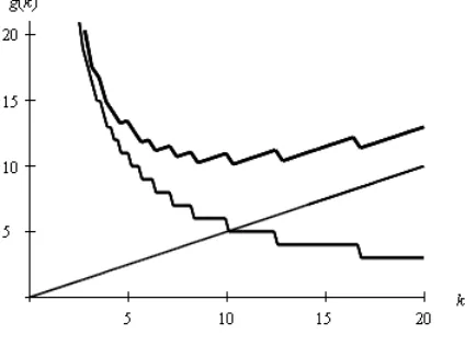
In this paper we present a polynomial-time algorithm which calculates an integer 1≤kopt≤nwhich minimizes the function (4) for any fixed positive rational number
a. The shape of the graph of the function g(k) is shown in Figure 1.
Fig. 1 Functiong(k) and its two componentsakand§n k
¨
The paper is organized as follows. In Sections 2 and 3 properties of the function
g(k) =ak+§nk¨are derived. It is shown in Section 2 that the problem can be solved easily ifais an integer. Additionally some symmetry properties for the values§nk¨are derived. For non-integer valuesathe difficulties of calculating a valuekopt∈ {1, . . . , n}
which minimizes g(k) arise because g(k) is oscillating in a neighborhood of kopt. In
Section 3 this oscillation behavior is studied in detail. It leads to a polynomial-time algorithm which is derived in Sections 4 and 5. In Section 6 it is shown that the running time of this algorithm isO(log3n). Section 7 contains some concluding remarks.
2 Symmetry and reduction to the casea >1
In this section we first show that it is easy to minimize
g(k) =ak+ln
k
[image:4.595.141.353.285.443.2]ifais a non-negative integer. Then for non-integer positive valuesawe reduce the case
a <1 to the casea >1 by using some symmetry properties of the values§n k
¨
. To calculate a value kopt which minimizes the function g(k) if a is integer we
consider the continuous function
f(k) =ak+n
k.
The functionsf andghave the following properties:
– f(k) is strictly decreasing (increasing) fork < pna (k > pna) and reaches its minimum if k=pna,
– g(k) =ak+§n k
¨
=§ak+n k
¨
=⌈f(k)⌉holds for integera. Using these two properties we have for allk≤¥pna
¦
f³jqnak´≤f(k) and therefore
g³jqnak´=lf³jqnak´m≤ ⌈f(k)⌉=g(k).
Similarly it can be shown that
g
³lq
n a
m´
≤g(k) for allk≥lqna
m
.
Thus,
kopt=
¥pn
a
¦
, if g¡¥pna¦¢≤g¡§pna¨¢,
§pn
a
¨
, otherwise.
From now on letabe a positive non-integer number.
Definition 1 Integer valuesKiare defined recursively as follows:
– K1= 1;
– given Ki, letKi+1be the integerw with Ki<w≤n, such that§nν¨=§νn−1
¨
for
ν=Ki+ 1, . . . ,w−1, and
§n
w
¨
6
=§wn−1
¨
.
Let r be the number of allKi-valuesK1, . . . , Kr =n. Notice, that the function
g(k) is strictly increasing in the interval [Ki, Ki+1−1]. Therefore, one can restrict to
theKi-values when searching for an integer value koptminimizing the functiong.
The following theorem describes an important symmetry relation between theKi
-values and§ni¨-values.
Theorem 1 There exists a symmetry relation between the valuesKi and Kr−i+1 of
the form:
Ki=
»
n Kr−i+1
¼
fori= 1, . . . , r. (5)
Equivalently,
Kr−i+1=
»
n Ki
¼
fori= 1, . . . , r (6)
Before proving Theorem 1 we derive some useful properties. For all positive integersjthe inequality
1
j+ 1− 1
j+ 2= 1
(j+ 1)(j+ 2) ≤ 1
j(j+ 1)= 1
j−
1
j+ 1 holds, which implies the inequality
n j+ 1−
n j+ 2 ≤
n j −
n
j+ 1 for allj≥1. (7)
Lemma 1 If lnjm=lj+1n m, then§nν¨−§ν+1n ¨≤1for allν≥j . Proof Assume that§nν¨−§ n
ν+1
¨
>1 , i.e., §nν¨−§ n ν+1
¨
≥2 for someν > j. Then
n ν −1≥
ln
ν
m
−2≥l n
ν+ 1
m
≥ν+ 1n
or
n ν −
n ν+ 1≥1. Furthermorelnjm=lj+1n mimplies
n j −
n j+ 1 <1. Together with (7) we have the contradiction:
1≤n
ν− n ν+ 1≤
n ν−1−
n ν ≤ · · · ≤
n j −
n j+ 1<1.
⊓ ⊔
Definition 2 The indextis defined as the largest index such thatKν=Kν−1+ 1 for ν= 2, . . . , t.
Observe that
Kν=ν forν= 1, . . . , t
and ln ν m < l n
ν−1
m
forν= 2, . . . , t,
ln
t
m
=l n
t+ 1
m
. (8)
Furthermore, due to Lemma 1
l n Kν m = » n Kν+1
¼
+ 1 for allν≥t. (9)
Lemma 2 Fori= 1, . . . , r−t+ 1the equality »
n Kr−i+1
¼
=i (10)
Proof Due to (9) and Definition 1 of theKν-values
»
n Kr−i
¼
=
»
n Kr−i+1
¼
+ 1 holds for alliwithr−i≥t. Thus, by induction we have
»
n Kr−i+1
¼
=i for alliwithr−i≥t−1, i.e.,i≤r−t+ 1
becauselKnrm= 1. ⊓⊔
Lemma 3 Fori= 1, . . . , r−t+ 1the equality ln
i
m
=Kr−i+1
is valid.
Proof By Definition 1 of theKν-values we have
»
n Kr−i+1
¼
6
=
»
n Kr−i+1−1
¼
which together with (10) implies
»
n Kr−i+1−1
¼
> i. With
n Kr−i+1 ≤
»
n Kr−i+1
¼
=i and n
Kr−i+1−1> i
we conclude
Kr−i+1−1<n
i ≤Kr−i+1or
ln
i
m
=Kr−i+1.
⊓ ⊔
Lemma 4 r−t < t and therefore lr
2
m
≤t.
Proof Assume thatr−t≥t. Then
»
n Kr−t+1
¼
=t=Kt=
l n
r−t+ 1
m
, (11)
where the first equality holds due to Lemma 2 takingi=t,the second equality holds due to Definition 2 and the third equality holds due to Lemma 3 takingi=r−t+ 1.
On the other hand, by Definition 2
ln
t
m
=l n
t+ 1
m
,
which together withr−t+1≥t+1 impliesKr−t+1> r−t+1 orKr−t+1−1≥r−t+1.
Together with Definition 1 we have:
»
n Kr−t+1
¼
<
»
n Kr−t+1−1
¼
≤lr n −t+ 1
m
,
Lemma 5 Fori=r−t+ 1, . . . , tthe equality
Ki=
»
n Kr−i+1
¼
holds.
Proof First we observe that in accordance with Lemma 4
r−t+ 1≤t,
so that
r−t+ 1 =Kr−t+1.
It follows that »
n Kt
¼
Lemma 2
= r−t+ 1 =Kr−t+1
and »
n Kr−t+1
¼
=l n
r−t+ 1
mLemma 3
= Kt.
The statement of Lemma 5 now follows from the relations:
Kr−t+1 =Kr−t+ 1, Kr−t+2=Kr−t+1+ 1, . . . , Kt=Kt−1+ 1,
l n Kt m < l n Kt−1
m
< · · · <
l
n Kr−t+1
m
together with the equalities
»
n Kt
¼
=Kr−t+1 and
»
n Kr−t+1
¼
=Kt.
⊓ ⊔
Proof of Theorem 1The proof is based on the above lemmas and equality
Ki=i fori= 1, . . . , t.
By Lemma 4 we have r−t+ 1≤t. Therefore, condition (5) holds due to Lemma 2 fori= 1, . . . , r−t, due to Lemma 5 for i=r−t+ 1, . . . , t, and due to Lemma 3 for
i=t+ 1, . . . , r. ⊓⊔
In what follows we demonstrate that if 0< a <1, then the problem of minimizing function gcan be reduced to a symmetric problem witha >1. For this purpose, we indicate that the functiong depends on the parameter adenoting the functiong by
ga. We have to find an indexi∗such thatKi∗ minimizesga(Ki) =aKi+
l
n Ki
m
for all
i= 1, . . . , r. Due to Theorem 1
Ki=
»
n Kr−i+1
¼
fori= 1, .., ror
»
n Ki
¼
=Kr−i+1 fori= 1, .., r.
Therefore fora >0 we have
ga(Kr−i+1) =aKr−i+1+
l
n Kr−i+1
m
=alKn
i m
+Ki
=a
³
1
aKi+
l
n Ki
m´
=ag1
a(Ki).
Thus, with (12) the Case 0< a <1 can be reduced to the Casea >1. One has to find
Ki∗ such thatg1
a(Ki∗) (where
1
a >1) is minimal. ThenKr−i∗+1=
l
n Ki∗
m
provides an optimal solutionga
³l
n Ki∗
m´
forga.
Now we derive an estimate on the valuer of the possibleKi-values.
Lemma 6 The value ofr is either 2s or 2s−1 with a unique integer s≤t defined from the condition: r
n+1 4−
1 2 ≤s <
r
n+1 4+
1 2.
Proof Conditionr= 2simplies together with Lemma 4 thats=r2 < t. Thus
s=KsTheorem 1=
»
n Kr−s+1
¼
=
»
n K2s−s+1
¼
=
»
n Ks+1
¼
Definition 2
= l n
s+ 1
m
.
Therefores−1<s+1n ≤sor
r
n+1 4−
1 2≤s <
√ n+ 1.
Observe that√n+ 1<
q
n+14+12.
Ifr= 2s−1 for somes, then we haves=Ks. Indeed, by Lemma 4
t≥lr2m=ls−12m≥s−12,
which implies
s≤t
sinces andtare integer. The latter inequality together with Definition 2 oftimplies
s=Ks. By Theorem 1
s=Ks=
»
n Kr−s+1
¼
=
»
n K2s−1−s+1
¼
=l n
Ks
m
=ln
s
m
,
which impliess−1<ns ≤sor
√ n≤s <
r
n+1 4+
1 2. Observe that
q
n+14−12≤√n. ⊓⊔
To find an integer 1≤i∗≤r such thatKi∗ minimizesgwe now assume thatais a non-integer number witha >1. As we show in the following lemma, the search for
i∗can be limited to the range {1,2, . . . , h1}withh1≤tsince the sequenceKh1+1<
Kh1+2<· · ·< Kris increasing.
Lemma 7 Ifa >1thenKi∗∈ {1, . . . , h1}where h1=
½
s, if § n s+1
¨
=§n s
¨
, s+ 1,otherwise.
Proof Due to Definition 2 oftwe haveKi=Ki−1+ 1 fori= 2, . . . , t. Together with
Theorem 1 this implies
»
n Kr−i+1
¼
=Ki=Ki−1+ 1 =
»
n Kr−i+2
¼
+ 1 fori= 2, . . . , t.
Becausea >1, this implies
g(Kν−1)−g(Kν) =aKν−1+
»
n Kν−1
¼
−aKν−
l n
Kν
m
≤ −a+
µ»
n Kν−1
¼
−lKn
ν
m¶
= =−a+ 1<0
forν=r−t+ 2, . . . , r, or
g(Kr−t+1)< g(Kr−t+2)<· · ·< g(Kr).
Due to Lemma 4 the inequalityt≥§r2
¨
holds, which implies
r−t≤r−l2rm≤r−r2 =r 2 and therefore
r−t+ 1≤ r 2+ 1
Lemma 6
≤ 22s+ 1 =s+ 1. (13)
We are on the safe side if we look for a valueKi∗ such thatg(Ki∗) is a minimum of
{g(Kν)|ν= 1,2, . . . , s+ 1}.
Notice that by Lemma 6
s≤t. (14)
Nowh1can be calculated by the following procedure.
If§s+1n ¨6=§ns¨, thens6=tand therefore by (14)s+ 1≤t. Thus, we set
h1:=s+ 1.
Otherwises=tand we can set
h1:=s.
⊓ ⊔
Notice that due to the above lemma we have
Ki=i
for all relevanti-values. For this reason in what follows we useiinstead ofKi.
Lemma 7 immediately implies an O(√n)-time algorithm just by calculating h1
3 Oscillation
The results of the previous section imply that the case of integerais easily solvable and for the non-integer case one may considera >1. From now on we assume thatais non-integer and greater than 1. The difficulties to find a positive non-integerkopt minimizing
the function g for non-integer values a arise because g is usually oscillating in the area around the optimal solution valuekopt. In this section we first present a general
description of the oscillating behavior of functiongand then proceed with details and justification.
Consider differences
∆i=
l n
i−1
m
−lnim (15)
which characterize the changes in the values of functiong:
g(i−1)−g(i) =∆i−a.
As we show later in this section,∆-values mainly decrease, but they may occasion-ally increase by 1:
∆j≤∆i+ 1 for all 1< i < j.
The increase/decrease structure of∆-values has some important structural properties. Consider the subsequence∆2,. . . ,∆h1 which contains an optimumkopt.
- The first∆jvalues are large and if∆j>⌈a⌉, then functiongis strictly decreasing.
- When ∆j achieves ⌊a⌋ for the first time for some j = l, the values of ∆j start
alternating between ⌈a⌉ and ⌊a⌋ and function g is oscillating (increasing when
∆j=⌊a⌋and decreasing when∆j=⌈a⌉).
- The oscillation range of∆-values ends after∆j changes to⌈a⌉for the last time for
somej=h−1, all subsequent∆-values are less than or equal to⌊a⌋and function
gis strictly increasing.
This means that the range{1, . . . , h1}can be narrowed to a smaller range{l, . . . , h}
with 1≤l≤h≤h1and within that range∆j∈ {⌈a⌉, ⌊a⌋}. We use notationA1=⌈a⌉
for the ∆j-value which leads to a decrease ing and andB1 =⌊a⌋ for the ∆j-value
which leads to an increase ing.
As we show later in this section, there is a certain regularity in the pattern ofA1
andB1. In particular,
(i) subsequence∆l, . . . , ∆hstarts with B1A| {z }1. . . A1B1A| {z }1. . . A1. . . B1A| {z }1. . . A1
con-sisting of repeatedA1. . . A1separated by a singleB1;
(ii) the next part is of the formB1A1. . . B1A1with single occurrences ofB1 alternat-ing with salternat-ingle occurrences ofA1;
(iii) the final part B1. . . B1
| {z }A1B| {z }1. . . B1A1. . . B| {z }1. . . B1A1 consists of repeated
B1. . . B1separated by a singleA1.
the blocksA2andB2of level 2 are alternating in a manner described by (i)-(iii) with the first partB2A| {z }2. . . A2B2A| {z }2. . . A2. . . B2A| {z }2. . . A2followed byB2A2. . . B2A2and then byB2. . . B2
| {z }A2B| {z }2. . . B2A2. . . B| {z }2. . . B2A2. Again, the search can be limited to
a smaller subsequence ∆l′, . . . , ∆h′ (l ≤ l′ ≤ h′ ≤ h) corresponding to a part of ∆l, . . . , ∆h.
The process of grouping several lower level blocks into higher level blocks and narrowing the boundaries of the search continues iteratively until at some level there are no blocks in-between the left and the right boundaries. Since any higher level block consists of at least 2 lower level blocks, the overall number of levels is no more than log2n. In what follows we explain the described approach in detail justifying its
correctness.
First we derive some properties of the∆i-values.
Lemma 8 For integers1≤i < j < n andk≥1withj+k≤n
» n j ¼ − » n j+k
¼
≤lnim−li+nkm+ 1
holds.
Proof For each non-negative integerνwithj+ν+ 1≤ndue to (7)
n j+ν −
n j+ν+ 1 ≤
n i+ν−
n i+ν+ 1 holds. This implies
n j −
»
n j+k
¼
≤ nj −j+nk
=
µ
n j −
n j+ 1
¶
+
µ
n j+ 1−
n j+ 2
¶
+· · ·+
µ
n j+k−1−
n j+k
¶
≤³ni −i+ 1n ´+³ n
i+ 1−
n i+ 2
´
+· · ·+³ n
i+k−1−
n i+k
´
= n
i − n i+k ≤
ln
i
m
−i+nk.
Therefore, together withlnjm≤ n
j + 1 » n j ¼ − » n j+k
¼
≤nj + 1−
»
n j+k
¼
≤lnim−i+nk+ 1,
i.e. » n j ¼ − » n j+k
¼
≤lnim−i+nk+ 1. In the previous inequality n
i+k is the only possible non-integer value. Hence it can be
replaced by§i+nk¨, which proves the lemma. ⊓⊔
Lemma 9 ∆j ≤ ∆i+ 1for all1< i < j.
Proof Application of Lemma 8 withk= 1 andireplaced byi−1 as well asjreplaced
Lemma 10 Letj≤h1be a positive integer. Then the following statements are correct.
(a) If∆j>⌈a⌉theng(ν−1)> g(ν)for all2≤ν≤j.
(b) If∆j<⌊a⌋theng(ν)> g(ν−1)for allh1≥ν≥j.
(c) If∆j=⌈a⌉theng(j) =g(j−1)−(⌈a⌉ −a), i.e.gdecreases by d=⌈a⌉ −a.
(d) If∆j=⌊a⌋theng(j) =g(j−1) + (a− ⌊a⌋), i.e.gincreases bye=a− ⌊a⌋.
Proof (a) By Lemma 9 for allν < j we have ∆j ≤∆ν+ 1. Furthermore,∆j >⌈a⌉
implies∆j≥ ⌈a⌉+ 1. Therefore
g(ν−1)−g(ν) =a(ν−1) +lνn −1
m
−aν−§n
ν ¨
= =∆ν−a≥∆j−1−a≥(⌈a⌉+ 1)−1−a >0.
(16)
(b) By Lemma 9 for allj≤νwe have∆ν≤∆j+ 1. Furthermore,∆j <⌊a⌋implies
∆j+ 1≤ ⌊a⌋. Therefore
g(ν)−g(ν−1) =aν+§nν¨−a(ν−1)−§ n ν−1
¨
= =a−∆ν≥a−∆j−1≥a− ⌊a⌋>0.
(17)
(c) Forν=j(16) providesg(j−1)−g(j) =∆j−a=⌈a⌉ −a.
(d) Forν=j(17) providesg(j)−g(j−1) =a−∆j =a− ⌊a⌋.
⊓ ⊔
Notice that the statements of Lemma 10 need not to be true ifj > h1because for
j > t≥h1 the equality Kj+1 =Kj+ 1 does not hold. Therefore one has to restrict
the search forkopt to the range 1, . . . , h1. Remember, we have no efficient algorithm
to calculatet.
Let l ≤h1 be the smallest positive integer with∆l ≤ ⌊a⌋. We may assume that
such an l always exists; otherwise∆j >⌊a⌋, i.e.,∆j ≥ ⌈a⌉ for all j≤h1, so thatg
decreases in [1, h1] andkopt=h1. Furthermore,∆j >⌊a⌋for at least onej; otherwise
∆j≤ ⌊a⌋for allj≤t, so thatgincreases in [1, h1] andkopt= 1.
Let hbe the smallest integer with ∆ν ≤ ⌊a⌋ for all ν, h ≤ ν ≤ h1. If such an
integer does not exist, we set h=h1. Clearlyl≤h and an optimal solution can be easily identified ifl∈ {h−1, h}. Therefore it remains to consider the casel < h−1.
By Lemma 9 we have
∆ν∈ {⌊a⌋,⌈a⌉} for allν=l, . . . , h−1.
We study the structure of the oscillation area defined by the sequence
∆l, ∆l+1, . . . , ∆h−1. We represent it as a sequence of repeated blocks of∆-values of
two typesAandB.Level 1 blocksA1 andB1are of the form
A1=⌈a⌉, B1=⌊a⌋.
More complexlevel λblocks AλandBλ,λ= 2,3, ..., are defined inductively. Each of these blocksAλorBλ consists of several blocksAλ−1 andBλ−1.
The following lemma describes the structure of the sequence ∆l, ∆l+1, . . . , ∆h−1
Lemma 11 The oscillation area has the form
∆l
B1 A1. . . A1
| {z }B1A| {z }1. . . A1 . . . B1| {z }A1. . . A1 B1A1B1A1. . .
m1 m2 ms
∆h−1 . . . B1A1B| {z }1. . . B1. . . A1| {z }B1. . . B1A1B| {z }1. . . B1 A1
ms m2 m1
(18)
where the block marked with ms(ms) corresponds to the last (first) occurrence of two
or moreA’s (B’s),
mv≤mu+ 1 for 1≤u < v≤s,
and
mv≤mu+ 1 for 1≤v < u≤s.
The structure (18) can be described informally as follows. At the beginning of the oscillation area subsequences of consecutive level 1 blocksA1are separated by a single
B1. Symmetrically, at the end of the oscillation area subsequences of consecutive level 1 blocksB1are separated by a singleA1.miandmidenote the number of repetitions of
A1 subsequences andB1 subsequences, respectively. If the middle part is non-empty, then it consists of alternating single occurrences ofA1- andB1-blocks. In what follows we prove that (18) correctly represents the oscillation area.
Proof The proof is split into 2 parts.
Part (a). First we claim that a subsequence of the form
∆i ∆i+1 ∆j∆j+1
. . . B1 B1 . . . A1 A1 . . . (19)
is not possible. Indeed, in this case we would have (with Lemma 8)
2⌈a⌉=∆j+∆j+1=
µ»
n
j−1
¼
−
»
n
j
¼¶
+
µ»
n
j
¼
−
»
n
j+1
¼¶
=
»
n
j−1
¼
−
»
n
j+1
¼
≤
»
n
i−1
¼
−
»
n
i+1
¼
+ 1 =∆i+∆i+1+ 1 = 2⌊a⌋+ 1 = 2⌈a⌉ −1
which leads to the contradiction 0≤ −1.
Due to the fact that a subsequence (19) is not possible to the left of anA1A1. . . A1 -block of length at least two, allA1. . . A1-blocks must be separated by a singleB1and to the right of aB1B1. . . B1-block of length at least two allB1. . . B1-blocks must be separated by a singleA1.
Part (b). Now assume thatmv≥mu+ 2 for some 1≤u < v≤s. Let∆i and∆i+k
be the∆’s corresponding to theB-bounds of theA-block of length ofmu and let∆j
correspond to the first A1 in the A-block of length mv, i.e., we have the following
situation:
∆i ∆i+k ∆j. . . ∆j+k. . . ∆j+k+z
. . . B1A1. . . A1
| {z } B1 . . . B1 |A1 . . . A{z1 . . . A1} B1. . .
wherez≥0. Again Lemma 8 leads to the contradiction:
(k+ 1)⌈a⌉=∆j+∆j+1+· · ·+∆j+k=
»
n
j−1
¼
−
»
n
j+k
¼
≤
»
n
i−1
¼
−
»
n
i+k
¼
+ 1 =∆i+∆i+1+· · ·+∆i+k+ 1
= (k−1)⌈a⌉+ 2⌊a⌋+ 1 = (k+ 1)⌈a⌉ −1.
Thus,mv< mu+ 2, i.e.mv≤mu+ 1 for 1≤u < v≤s. Symmetrically, it can be
shown thatmv≤mu+ 1 for 1≤v < u≤s. ⊓⊔
Consider an oscillation area of the form (18) where byA1the functiongis decreased by the valuedand by B1the functiongis increased by the valuee, see Lemma 10.
Ifd=ethen the subsequences
B1A| {z }1. . . A1 withmi≥2
mi
in the left part of the oscillation area decreaseg. The subsequences
A1B1. . . B1
| {z } withmi≥2
mi
in the right part of the oscillation area increase g. The subsequences A1B1 in the middle part do not changeg. Therefore an optimal solution is given by the end of the lastB1A| {z }1. . . A1 subsequence withmi≥2 occurrences ofA1.
It remains to consider the cased < e(the casee < dis treated symmetrically). In this case an optimal solution can be found in
B1A1. . . A1
| {z }B1A| {z }1. . . A1. . . B1A| {z }1. . . A1
m1 m2 ms
(20)
Letl′≤sbe the smallest positive integer withml′d≤e, i.e.,ml′ ≤
¥e
d
¦
. We may assume that such anl′ exists because otherwisegachieves its minimum at the end of sequence (20). Furthermore,mi >
¥e
d
¦
for at least one i; otherwise the minimum is achieved just before the oscillation area, i.e., it is given by the last position before the oscillation area.
Let h′ be the smallest positive integer with mν ≤ ¥ed¦ for all ν ≥ h′. By the
definition of l′ the function g is strictly decreasing for all mν withν < l′ and
non-decreasing for all mν with ν ≥ h′ (because in the latter case mν ≤ ¥de¦ ≤ ed or
e ≥ mνd). Clearly, l′ ≤ h′ and an optimal solution can be easily identified if l′ ∈
©
h′−1, h′ª. Therefore it remains to consider the casel′< h′−1. With Lemma 11
mν∈
nje
d
k
,le d
mo
for alll′ ≤ν≤h′−1. (21) Define
A2=B1A1. . . A1
| {z }§ and B2=B1A| {z }1. . . A1.
e d
¨ ¥e
d
Notice, that by the blockA2(B2) the functiongis decreased (increased) by
d′=le
d
m
d−e≥edd−e= 0 (e′=e−jedkd≥e−ded= 0). (23) In what follows we will show that the new (considerably smaller) oscillation area
B1A| {z }1. . . A1B1| {z }A1. . . A1. . . B1A| {z }1. . . A1
ml′ ml′+1 mh′−1
has the form
B2 A2. . . A2
| {z }B2A| {z }2. . . A2 . . . B2| {z }A2. . . A2 B2A2B2A2. . .
m′1 m′2 m′s′
. . . B2A2B2. . . B2
| {z }. . . A2 B| {z }2. . . B2 A2B| {z }2. . . B2A2
m′s′ m′2 m′1
where m′s′, ms′′ ≥ 2, m′j ≤ m′i + 1 for 1 ≤ i < j ≤ s′, and m′j ≤ m′i+ 1 for 1≤j < i≤s′.
Notice, that level 2 blocks are sequences of level 1 blocks. This process will be iter-ated considering level 2 blocksA2andB2instead ofA1andB1, etc. More specifically, given levelλblocksAλandBλ, whereAλ(Bλ) decreases (increases)gbydλ(eλ), the blocks in levelλ+ 1 are defined as
Aλ+1=BλAλ. . . Aλ
| {z }l and Bλ+1=Bλ A| {z }λ. . . Aλ.
eλ dλ
m j
eλ dλ k
Then by the blockAλ+1 (Bλ+1) the functiongis decreased (increased) by
dλ+1=
»
eλ dλ
¼
dλ−eλ≥ e
λ
dλd λ
−eλ= 0 (eλ+1=eλ−
¹
eλ dλ
º
dλ≥eλ−e
λ
dλd
λ= 0). (24)
Later we will show that to identify Kopt one has to consider at most O(logn)
levels.
The next theorem generalizes Lemma 11.
Theorem 2 The oscillation area in each levelλhas the form
∆l
BλA| {z }λ. . . Aλ BλA| {z }λ. . . Aλ. . . Bλ A| {z }λ. . . AλBλAλBλAλ. . .
mλ1 mλ2 mλsλ
∆h−1 . . . BλAλB| λ. . . B{z λ}. . . Aλ |Bλ. . . B{z λ}AλB| λ. . . B{z λ} Aλ
mλsλ mλ2 mλ1
(25)
where
mλsλ, mλsλ ≥2,
mλv ≤mλu+ 1 for 1≤u < v≤sλ,
Proof We prove the theorem by induction byλ-values. Due to Lemma 11 the theorem is correct for levelλ= 1. For the induction step we follow the structure of the proof of Lemma 11.
Part (a). Consider the oscillation area at a level λ+ 1, λ ≥1 consisting of blocks
Aλ+1 = BλAλ. . . Aλ with ledλλ m
repetitions ofAλ and Bλ+1 = BλAλ. . . Aλ with
j
eλ
dλ k
repetitions ofAλ:
Aλ+1=BλA| {z }λ. . . Aλ
l
eλ dλ
m
, Bλ+1=BλA| {z }λ. . . Aλ
j
eλ dλ
k
(26)
Again a subsequence
. . . Bλ+1Bλ+1. . . Aλ+1Aλ+1. . . (27) is not possible. Indeed (27) has the form
BλA
i′
λ. . . Aλ
| {z }
Bλ+1
BλAλ. . . Aλ
j′
| {z }
Bλ+1
Bλ. . . BλAλi′A+ρλ. . . Aλ
| {z }
Aλ+1
BλAλ. . . A
j′+ρ λAλ
| {z }
Aλ+1
. (28)
Let i′ be the index of the first∆ν in the firstAλ of the firstBλ+1, i.e., the first
position in this firstAλ. Letj′be the last position of the lastAλof the secondBλ+1. Furthermore leti′+ρbe the first position of the secondAλ inAλ+1 in (28). Notice that the sequences ∆i′. . . ∆j′ and ∆i′+ρ. . . ∆j′+ρ are identical. Let i < i′ be the
largest index with∆i 6= ∆i+ρ and ∆ν =∆ν+ρ forν =i+ 1, . . . , i′. Such an index
exists because blockBλ is the block preceding immediately positioni′ inBλ+1 and
Aλis the block preceding immediately positioni′+ρinAλ+1(see (28)). Furthermore,
∆i+ρ=⌈a⌉and∆i=⌊a⌋. To show this, we decomposeAλandBλ into blocksAλ−1
andBλ−1:
Bλ= Bλ−1 Aλ−1. . .Aλ−1, Aλ= Bλ−1 Aλ−1 Aλ−1. . .Aλ−1.
It is easy to see that only the first fragments of the above sequences are different while the final parts are the same. We continue the decomposition into lower level blocks:
Bλ= Bλ−2Aλ−2. . .Aλ−2 Aλ−1. . .Aλ−1, Aλ= Bλ−1Bλ−2 Aλ−2Aλ−2. . .Aλ−2 Aλ−1. . .Aλ−1.
Proceeding in a similar way we obtain:
Bλ= B1 A1. . .A1 A2. . .A2. . .Aλ−2. . .Aλ−2
Aλ= Bλ−1Bλ−2. . .B1 A1A1. . .A1A2. . .A2. . .Aλ−2. . .Aλ−2 (29)
which proves the claim that∆i+ρ=⌈a⌉and∆i=⌊a⌋.
Let j > j′ be the smallest index with∆ν =∆ν+ρ forν =j′+ 1, . . . , j−1 and
∆j6=∆j+ρ. Again∆j=⌊a⌋and∆j+ρ=⌈a⌉. Now we have with Lemma 8
∆i+· · ·+∆j+ 2 =∆i+1+· · ·+∆j−1+ 2⌊a⌋+ 2
=∆i+1+ρ+· · ·+∆j−1+ρ+ 2⌈a⌉ (30)
=∆i+ρ+· · ·+∆j+ρ
Lemma 8
which provides the contradiction 2≤1.
Part (b). To prove that mλv+1 ≤ muλ+1 + 1 for 1 ≤ u < v ≤ sλ+1 assume that
mλv+1≥muλ+1+ 2 for some 1≤u < v≤sλ+1. Then similar to Part (b) in Lemma 11
we have the situation with the blocksAλ+1 andBλ+1in levelλ+ 1,λ≥1:
. . . Bλ+1 A|λ+1. . . A{z λ+1}
mλ+1
u
Bλ+1. . . Bλ+1Aλ+1|Aλ+1. . . A{z λ+1}
mλ+1
u
Aλ+1. . . Aλ+1
| {z }
mλ+1
v ≥mλu+1+2
Bλ+1. . .
Substituting lower level blocks instead of some ofAλ+1andBλ+1we rewrite the above sequence as follows:
. . .
Bλ+1
z }| {
BλAλ
i′ . . .A
λ
Aλ+1. . .Aλ+1
| {z }
mλ+1
u
Bλ+1
z }| {
BλAλ. . .Aλ
j′ . . . B
λ+1
Aλ+1
z }| {
BλAλAλ
i′+ρ. . .A λ
Aλ+1. . .Aλ+1
| {z }
mλ+1
u
Aλ+1
z }| {
BλAλ. . .AλAλ
j′+ρ A λ+1
. . .Aλ+1
| {z }
mλ+1
v −mλu+1−1
Bλ+1. . . (31)
Definition of indicesi′,j′andiandjis similar to that in part (a). Namely, leti′be the index of the first∆ν in the firstAλof the firstBλ+1, i.e., the first position in this
firstAλ. Let j′ be the last position of the lastAλ of the secondBλ+1. Furthermore let i′+ρ be the first position of the second Aλ inAλ+1 (see (31)). Notice that the sequences∆i′. . . ∆j′ and∆i′+ρ. . . ∆j′+ρ are identical. Leti < i′ be the largest index
with∆i 6=∆i+ρ and ∆ν =∆ν+ρ forν =i+ 1, . . . , i′. Such an index exists because
blockBλis the block preceding immediately position i′ inBλ+1and Aλ is the block preceding immediately position i′+ρ inAλ+1 (see (31)). Furthermore, as shown in Part (a),∆i+ρ=⌈a⌉and∆i=⌊a⌋. Letj > j′be the smallest index with∆ν =∆ν+ρ
forν=j′+ 1, . . . , j−1 and∆j6=∆j+ρ.
We have
. . . Aλ
j′ B
λAλ. . .
. . . Aλ
j′+ρA λ. . .
By expandingBλAλ andAλ, which followAλ
j′ and A
λ
j′+ρ, respectively, we get BλAλ=Bλ−1Aλ−1. . . Aλ−1Bλ−1Aλ−1
Aλ =Bλ−1Aλ−1. . . Aλ−1Aλ−1
BλAλ=Bλ−1Aλ−1. . . Aλ−1Bλ−2Aλ−2. . . Aλ−2Bλ−2Aλ−2 Aλ =Bλ−1Aλ−1. . . Aλ−1Bλ−2Aλ−2. . . Aλ−2Bλ−2
.. .
Again∆j=⌊a⌋and∆j+ρ=⌈a⌉and the sequences
∆i+1, . . . , ∆j−1 and∆i+ρ+1, . . . , ∆j+ρ−1
are identical. Similar to Part (a), relation (30) holds leading to the contradiction 2≤1. Symmetrically one can provemλv ≤mλu+ 1 for 1≤v < u≤sλ. ⊓⊔ We introduce the following notations. A blockXλ(Xλ=AλorXλ=Bλ) at some arbitrary levelλcan be decomposed in a unique way into level 1 blocks∆ν∈ {⌈a⌉,⌊a⌋},
i.e.,
Xλ=∆i∆i+1. . . ∆j.
The cumulative∆-value ofXλis defined as
∆Xλ =
j
X
ν=i
∆ν=
³l n
i−1
m
−lnim´+³ln
i
m
−li+ 1n m´+· · ·+
+
µ»
n j−1
¼
−
»
n j
¼¶
=
l n
i−1
m
−
»
n j
¼
and its length is given by
lXλ=j−i+ 1.
The values of ∆Xλ and lXλ forXλ =Bλ andXλ =Aλ can be calculated level by
level using the recursive formulas which follow from (22) and (26):
∆Bλ =∆Bλ−1+
¹
eλ−1 dλ−1
º
∆Aλ−1, ∆Aλ =∆Bλ−1+
»
eλ−1 dλ−1
¼
∆Aλ−1 (32)
and
lBλ =lBλ−1+
¹
eλ−1 dλ−1
º
lAλ−1, lAλ=lBλ−1+
»
eλ−1 dλ−1
¼
lAλ−1 (33) with initial values
∆B1=⌊a⌋, ∆A1=⌈a⌉, lA1 =lB1= 1. (34) Due to Lemma 10 and (24) the valueseλ anddλare calculated recursively by
eλ=eλ−1−
¹
eλ−1 dλ−1
º
dλ−1 and dλ=
»
eλ−1 dλ−1
¼
dλ−1−eλ−1 (35)
with initial values
4 A Polynomial-Time Algorithm
In this section we formulate an algorithm for finding an integer 1≤kopt≤h1, which
minimizesgunder an assumption thata >1. The idea of our algorithm is to calculate for each relevant level the corresponding oscillation area. The levels λare considered one by one. In our description we assume that in the current levelλconditioneλ≥dλ
holds. The caseeλ< dλis symmetric and the corresponding version of the algorithm which takes care of both cases can be easily derived.
The algorithm stops when an oscillation area contains at most two blocks. In this casekoptcan be identified easily. The algorithm can be described by a recursive
pro-cedure Optimize(λ, l, h), wherel is a lower bound and his an upper bound for the oscillation area at levelλ.
Procedure Optimize(λ, l, h)
1. If λ≥2then h:=Rightboundary(λ−1, l, h); 2. l:=Updateleft(λ, l, h);
3. h:=Updateright(λ, l, h);
4. Calculate the blocksXlλ+1 andXhλ+1, which can be of typeAλ+1orBλ+1at level
λ+ 1 in whichlandhare contained;
5. Ifat least one (λ+1)-block exists betweenXlλ+1andXhλ+1,then Optimize(λ+1,
l, h)
6. else CalculateOptimum³λ+ 1, Xlλ+1, Xhλ+1´
Rightboundary(λ−1, l, h) provides an upper bound for the right boundary of the oscillation area for λ ≥ 2. Such a boundary is provided by the last position of the last Aλ−1Aλ−1-subsequence in an oscillation area at levelλ−1. The procedure
Updateleft(λ, l, h) andUpdateright(λ, l, h) calculate the left boundarybland right boundary bh of the oscillation area at the next higher level, given a lower bound l
forbland an upper boundhforbh. Notice, that Rightboundary(λ, l, h) and Upda-teright(λ, l, h) withλ≥2 are different procedures.Rightboundary(λ, l, h) identifies the last position of the lastAλAλ-subsequence in an oscillation area at levelλwhich defines the inputhfor the procedureUpdateright(λ, l, h).Rightboundary(λ, l, h) is needed to cut off theBλAλBλAλ· · ·AλBλ· · ·BλAλ-part which under the assumption
eλ≥dλis not relevant for identifying an optimal solution.
The procedureCalculateOptimum³λ, Xlλ, Xhλ´ provides an optimal solution if only one block Xlλ=Xhλ or two adjacent blocksXlλ andXhλ are left. If Xlλ andXhλ
coincide and are equal toBλ, thenk−1 provides an optimal solution where kis the first index inXlλ. IfXlλ and Xhλ coincide and are equal to Aλ, then the last index inXlλ provides an optimal solution. IfXlλ andXhλ are two adjacent blocks, then for
XlλXhλwe have the four cases:AλAλ,AλBλ,BλAλ, andBλBλ. In the last two cases againk−1 provides an optimal solution wherekis the first index inXlλ. In CaseAλAλ
the last index inXhλprovides an optimal solution and in CaseAλBλthe last index in
Xlλ provides an optimal solution.
Minimize gis the main procedure which calculatesKopt.
Minimize g
1. l:= 1;h:=h1; 2. λ:= 1;
In the first iteration of Minimize g the procedure Optimize(1,1, h1) is called in which l and h are calculated by Updateleft(1,1, h1) and Updateright(11, h1), respectively. Due to Lemma 11, the search can be narrowed to the subsequence
∆l, . . . , ∆h−1, marked by (18), with ∆l corresponding to the first occurrence of B1
and∆h−1corresponding to the last occurrence ofA1. This is depicted in (20)
z }| {
B1
z }| {
A1. . .A1. . .B1
z }| {
A1. . .A1B1A1. . .B1A1
z }| {
B1. . .B1A1. . .
z }| {
B1. . .B1A1
l l l
∆2. . . ∆l · · · ∆h′ · · · ∆h−1
| {z }∆h. . .∆h1
Ifl < h−1 thenOptimize(2, l, h) is called which first callsRightboundary(1, l, h) to find the last positionh′ of the last subsequenceA1A1. Now the level 2 starts which is restricted to the range∆l, . . . , ∆h′ marked by (20).
Next we describe the procedures Updateleft(λ, l, h) and Updateright(λ, l, h), which by binary search provides the beginning and end of the oscillation area at level
λ+ 1;£l′, l′′¤and £h′, h′′¤are the corresponding search intervals. The description of
Updateleft(λ, l, h) and Updateright(λ, l, h) for λ= 1 differs slightly from the de-scription forλ >1.
First we formulate Updateleft(λ, l, h) for λ= 1, afterwards we describe Upda-teright(λ, l, h) forλ= 1 and finally the update procedures forλ >1.
Procedure Updateleft(1,1, h1) 1. l′:= 1;l′′:=h1;∆1:=∞; 2. Whilel′′≥l′+ 2do
3. j:=jl′+2l′′k;
4. If ∆j>⌈a⌉thenl′:=j;
5. If ∆j≤ ⌊a⌋thenl′′:=j;
6. If ∆j=⌈a⌉then
7. Find the maximal⌈a⌉-block
∆j′ ∆j ∆j′′ ⌈a⌉. . .⌈a⌉. . . ⌈a⌉
containing∆j;
8. If ∆j′′+1>⌈a⌉thenl′:=j′′+ 1; 9. If ∆j′′+1≤ ⌊a⌋then
10. if j′′+ 1< l′′thenl′′:=j′′+ 1
11. else if ∆j′−1>⌈a⌉then returnj′′+ 1
12. elsel′′:=j′−1;
13. Returnl′′
The procedure used in Step 7 for finding the maximal⌈a⌉-block to which∆jbelongs
will be discussed in Section 5.
If on the other hand ∆j′′+1 ≤ ⌊a⌋,l′′ ≤j′′+ 1 (which impliesl′′ =j′′+ 1), and ∆j′−1>⌈a⌉, then againl′′ marks the start of the oscillation area.
Notice, that Updateleft(1,1, h1) returns an indexl with∆l≤ ⌊a⌋. If ∆l <⌊a⌋
thenl−1 provides an optimal solution. Otherwise,∆l=⌊a⌋, i.e., lis the index of a
B-block.
The procedure Updateright(λ, l, h) forλ= 1 is shown below. It is symmetric to
Updateleft(λ, l, h) forλ= 1.
Procedure Updateright(1,1, h1) 1. h′:= 1;h′′:=h1;∆1:=∞; 2. Whileh′′≥h′+ 2do
3. j:=jh′+2h′′k;
4. If ∆j<⌊a⌋thenh′′:=j;
5. If ∆j≥ ⌈a⌉thenh′:=j;
6. If ∆j=⌊a⌋then
7. Find the maximal⌊a⌋-block
∆j′ ∆j ∆j′′ ⌊a⌋. . .⌊a⌋. . . ⌊a⌋
containing∆j;
8. If ∆j′−1<⌊a⌋thenh′′:=j′−1;
9. If ∆j′−1≥ ⌈a⌉then
10. if j′−1> h′ thenh′:=j′−1
11. else if ∆j′′+1<⌊a⌋then returnj′−1
12. elseh′:=j′′+ 1;
13. Returnh′
Updateright(1,1, h1) returns an index h with ∆h ≥ ⌈a⌉. If ∆h >⌈a⌉, then h
provides an optimal solution. Otherwise,∆h=⌈a⌉, i.e.his the index of anA-block.
Next we describeUpdateleft(λ+ 1, l, h) forλ≥1. The corresponding oscillation area has the form (25) where blockAλ decreases the objective functiongbydλ and block Bλ increases g byeλ. l is the first index in (25) and h is the last index. We assume that eλ ≥dλ. The case eλ ≤ dλ is treated symmetrically. In the caseeλ ≥ dλ the last occurrence of an Aλ. . . Aλ-block with at least two Aλ repeated defines a right boundary of the relevant BλAλ. . . Aλ-area. The blocksXλ+1 considered in
Updateleft(λ+ 1, l, h) forλ≥1 have the form
Xλ+1=BλAλ. . . Aλ
| {z }
mXλ+1
and its type depends on the number mXλ+1 of repetitions of Aλ.
Up-dateleft(λ+ 1, l, h) for λ≥1 is similar to Updateleft(1,1, h1), see the description below.
Procedure Updateleft(λ+ 1, l, h)
1. l′:=l;l′′:=h;
2. Calculate the blocksXlλ′+1 andX
λ+1
l′′ in which∆l′ and∆l′′ are contained; 3. l′:= the last index inXlλ′+1;l
′′:= the first index inXλ+1
l′′ ; 4. Whilea (λ+ 1)-block exists betweenXlλ′+1andX
λ+1
5. j:=jl′+l′′ 2
k
;
6. LetXjλ+1 be the block to which∆j belongs;
7. If mXλ+1
j > l
eλ dλ m
thenl′:= the last index inXjλ+1; 8. If mXλ+1
j ≤
j
eλ dλ k
thenl′′:= the first index inXjλ+1; 9. If mXλ+1
j
=leλ
dλ m
then
10. find the maximal sequence of repetitions of the blockXλ+1=Xjλ+1:
Cλ+1Xλ+1. . . Xλ+1
j . . . X
λ+1Dλ+1³Cλ+1, Dλ+1
6
=Xλ+1´;
11. If mDλ+1>
l
eλ
dλ m
then
replacel′ by the last index inDλ+1 and setXlλ′+1=D
λ+1;
12. If mDλ+1≤
j
eλ
dλ k
then
13. if the first index inDλ+1is smaller thanl′′
thenletl′′ be the first index inDλ+1and setXlλ′′+1=D
λ+1
14. else if mCλ+1 >
l
eλ dλ m
then returnthe first index inDλ+1
15. elsereplacel′′by the first index inCλ+1and setXlλ′′+1=C
λ+1;
17. Returnl′′
The procedure for identifying blockXjλ+1to which∆j belongs and for calculating
the first and last indices ofXjλ+1 will be discussed in Section 5.
Notice, that during the performance of the procedure Updateleft(λ+ 1, l, h) for
λ ≥ 1 the inequalities mXλ+1
l′′ ≤
j
eλ
dλ k
and mXλ+1
l′ >
l
eλ
dλ m
always hold. Therefore
Xlλ′′+1 is to the right and X
λ+1
l′ is to the left of the X
λ+1, . . . , Xλ+1-block. This
implies thatCλ+1andDλ+1 always exist.
The procedureUpdateright(λ+ 1, l, h) is symmetric toUpdateleft(λ+ 1, l, h). It remains to describe the procedureRightboundary(λ, l, h) which calculates the last position of the lastAλAλ-subsequence in an oscillation area at levelλ,λ≥2, if such a position exists. Again binary search is applied to find this position. More specifically, we calculate a positionj in a block in AλAλBλAλBλAλ. . .where AλAλ is the last occurrence of two consecutiveAλ. In the second step the last position inAλAλ must be calculated. This is easy if∆j belongs to AλAλ. Otherwise, the first occurrence of
BλAλ inAλAλBλAλBλAλ. . . Bλ
j A
λ must be identified. A corresponding method is
discussed in Section 5.3.
We start by calculating the last index h′ of the block containing l and the first indexh′′ of the block containing h. If there exists another block between these two blocks, we calculate the blockXjλ containingj:=
l
h′+h′′ 2
m
then the following three subcases are considered:
Case 1:
h′
AλBλ. . .AλBλAλBλ. . .Aλ
j
Bλ(the fragment∆h′, . . . , ∆j is covered by
AλBλ-sequences) Case 2: AλAλBλ. . .AλBλ(nearest repeatedAλwhich appear to the left ofXjλ) Case 3: BλBλAλBλ. . .AλBλ(nearest repeatedBλwhich appear to the left
ofXjλ) If Case 3 holds, then due to Part (a) in the proof of Theorem 2 there is no AλAλ -subsequence to the right ofXjλ. In this case we set h′′ equal to the first index in the
j-blockXjλ. In the other two cases noBλBλ-subsequence occurs to the left ofXjλbut anAλAλ-subsequence may occur to the right ofXjλand we seth′ equal the last index in thej-blockXjλ.
The caseXjλ=Aλ is treated symmetrically.
In either case we proceed with the new valuesh′andh′′and continue until there is no other block between theh′-block and theh′′-block. If both blocks areBλ-blocks then we sethequal toh′. Otherwise we sethequal toh′′. Now we have reached a situation in which noBλBλ occurs to the left of theh-block and we calculate the last position of the lastAλAλwhich occurs before theh-block. The algorithm is summarized below.
Procedure Rightboundary(λ, l, h) 1. h′:= last index of the block containingl; 2. h′′:= first index of the block containingh;
3. Whileat least one block exists between theh′-block and theh′′-blockdo
4. j:=lh′+h′′ 2
m
;
5. Xjλ= the block containing∆j;
6. If Xjλis aB-blockthen
7. if
BλBλAλBλ. . .Aλ
j
Bλ
8. then h′′:= the first index in thej-block Bλ
9. else h′:= the last index in thej-blockBλ
10. else if
BλBλAλBλ. . .AλBλ
j
Aλ
11. thenh′′:= the first index in thej-blockAλ
12. elseh′:= the last index in thej-blockAλ; 13. If Xhλ′ =Bλ andXhλ′′=Bλhold,thenh:=h
′
14. elseh:=h′′;
15. Returnthe last position of the lastAλAλ-block which does not end later than theh-block
Steps 13 and 14 are such that hbelongs to the block in the BλAλBλAλ. . .-area after the last occurrence of AλAλ. Notice that procedure Rightboundary always deals with the blocksXhλ′ and Xhλ′′ in different positions in the λ-oscillation area so that these two blocks never coincide.
5 Calculating Block Boundaries
In Step 7 of the procedureUpdateleft(1,1, h1) and in a corresponding step in Upda-teright(1,1, h1) one has to calculate the boundaries of anAA . . . A-block andBB . . . B -block, respectively. Similar calculations are needed for higher level Updateleft and
Updaterightprocedures. We also have to identify at the current levelλthe blockXjλ
in which ∆j is contained and to find the first and the last index of Xjλ. This is done
by first calculating the boundaries of the level 2 blocks in which∆j is contained, then
calculating the boundaries of the level 3 blocks in which∆j is contained, etc.
In the next two subsections it is shown how to calculateAλAλ. . . Aλ-block bound-aries for level λ = 1 and for higher levels λ. BλBλ. . . Bλ-block boundaries can be calculated in a similar way. We also need to calculate the boundaries of an
AλBλAλBλ. . . AλBλ-block. A corresponding procedure is described in the third sub-section.
5.1 Calculating Boundaries forAA . . . A-Blocks at Level 1
To calculate the left boundary of anAA . . . A-block at level 1 we consider the following two situations:
Case 1 : B A A . . . A
∆i−δ ∆i−δ+1∆i−δ+2. . . ∆i
Case 2 : D A A . . . A
∆i−δ ∆i−δ+1∆i−δ+2. . . ∆i
withA=⌈a⌉,B=⌊a⌋andD >⌈a⌉(cf. Lemma 9). In both cases
§ n
i−ν
¨
−§ni
¨
=¡§i−nν¨−§i−nν+1¨¢+¡§i−nν+1¨−§i−νn+2¨¢+... ...+§i−n1¨−§n
i
¨
=⌈a⌉ν forν= 0, ..., δ.
Thus,
l n
i−ν
m
=ξi+⌈a⌉ν forν= 0, ..., δ (37)
withξi=
§n
i
¨
holds. Additionally,
»
n i−(δ+ 1)
¼
=ξi+⌈a⌉δ+⌊a⌋=ξi+⌈a⌉(δ+ 1)−1 (38)
holds in Case 1 and
»
n i−(δ+ 1)
¼
=ξi+⌈a⌉(δ+ 1) +x withx≥1 (39)
holds in Case 2.
Proof The necessary part has just been proved. It remains to show that (37) and (38) ((37) and (39)) are sufficient for Case 1 (Case 2).
In Case 1 in which (37) and (38) hold, subtracting §i−nν¨ = ξi +⌈a⌉ν from
l
n i−(ν+1)
m
=ξi+⌈a⌉(ν+ 1) yields∆i−ν =⌈a⌉forν= 0, ..., δand∆i−(δ+1)=⌊a⌋.
In Case 2 in which (37) and (39) hold, a similar subtraction provides∆i−ν =⌈a⌉
forν= 0, ..., δand∆i−(δ+1)=⌈a⌉+xwithx≥1. ⊓⊔
We give a geometric interpretation of Cases 1 and 2. Consider first Case 1. Condition (37) is equivalent to
n
i−ν ≤ξi+⌈a⌉νand n
i−ν > ξi+⌈a⌉ν−1. (40)
Furthermore, (38) implies
n i−(δ+ 1) ≤
»
n i−(δ+ 1)
¼
=ξi+⌈a⌉(δ+ 1)−1. (41)
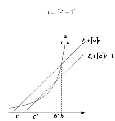
In this case the lineξi+⌈a⌉ν−1 intersects the hyperbola i−nν in one pointc
′=b′or two pointsc′< b′.
Furthermore, the interval£c′, b′¤contains the integer point δ+ 1 and c≤0 < c′
where in cthe line ξi+⌈a⌉ν intersects the hyperbola. The situation with c′ < b′ is
depicted in Figure 2.
To calculateδ one has to find the smallest solutionc′ of the equation
n
i−ν =ξi+⌈a⌉ν−1
which is equivalent to the quadratic equation
⌈a⌉ν2+ (ξi−1−i⌈a⌉)ν+n−i(ξi−1) = 0.
δis calculated by
δ=§c′−1¨ (42)
[image:26.595.145.332.441.637.2]Now consider Case 2 in which (37) and (39) are satisfied. Then besides (40) the
inequality »
n i−(δ+ 1)
¼
> ξi+⌈a⌉(δ+ 1)
holds. The hyperbola does or does not intersect the lower lineξi+⌈a⌉ν−1. In the
latter case, due to (40)c≤0< b, wherecandbare intersection points of the hyperbola and the upper lineξi+⌈a⌉ν, see Figure 2.
On the other hand, if the hyperbola intersects the lower lineξi+⌈a⌉ν−1, then
due to (40) eitherc≤0< c′ orb′ <0≤b, wherec′ andb′ are intersection points of the hyperbola and the lower lineξi+⌈a⌉ν−1. Observe that ifc≤0< c′, then due
to (39) and (40), interval£c′, b′¤ cannot contain an integer point. In both cases case
δ=⌊b⌋wherebis the largest solution of the equation
n
i−ν =ξi+⌈a⌉ν.
We conclude that in order to find out which case applies and to calculate the corresponding valueδone has to solve two quadratic equations.
The right boundary of anA...A-block can be calculated in a similar way.
5.2 Calculating Boundaries forAλAλ. . . Aλ-Blocks
We describe how to calculate the left boundary ofAλAλ. . . Aλ-blocks at some levelλ
2
7
Aλ-sequence : Bλ−1 Aλ−1 Aλ−1. . .Aλ−1Aλ. . . .Aλ Bλ−1 Aλ−1 Aλ−1. . .Aλ−1
Case 2 : Bλ−1Aλ−1. . .Aλ−1 Aλ−1 Aλ−1 Aλ−1. . .Aλ−1Aλ. . . .Aλ Bλ−1 Aλ−1 Aλ−1. . .Aλ−1
↑ i−lAλ(δ+1)
↑ j−lAλ(δ+1)
↑ i
↑ j
(43)
Bλ−1= B A. . .A A(2). . .A(2). . .Aλ−2. . .Aλ−2
Aλ−1= Bλ−2Bλ−3. . .B A A. . .A A(2). . .A(2). . .Aλ−2. . .Aλ−2 (44)
Case 1 : BA . . . A . . . Aλ−2. . . Aλ−2 Aλ−1. . . Aλ−1Aλ. . . Aλ Aλ-sequence : BA . . . A . . . Aλ−2. . . Aλ−2 Bλ−2. . . B AA . . . A . . . Aλ−2. . . Aλ−2 Aλ−1. . . Aλ−1Aλ. . . Aλ
Case 2 : Bλ−1Aλ−1. . .Aλ−1 Bλ−2. . .B AA . . . A . . . Aλ−2. . . Aλ−2 Bλ−2. . . B AA . . . A . . . Aλ−2. . . Aλ−2 Aλ−1. . . Aλ−1Aλ. . . Aλ
↑ ↑
i−lAλ(δ+1) j−lAλ(δ+1)
Case 1 (cont.) : BA . . . A . . . Aλ−2. . . Aλ−2 Bλ−2. . . BA A . . . A . . . Aλ−2. . . Aλ−2 Aλ−1. . . Aλ−1 Aλ-sequence (cont.) : BA . . . A . . . Aλ−2. . . Aλ−2 Bλ−2. . . BA A . . . A . . . Aλ−2. . . Aλ−2 Aλ−1. . . Aλ−1 Case 2 (cont.) : BA . . . A . . . Aλ−2. . . Aλ−2 Bλ−2. . . BA A . . . A . . . Aλ−2. . . Aλ−2 Aλ−1. . . Aλ−1
↑ ↑
i j
To calculate the block Bλ (Case 1) or Dλ (Case 2) at the left boundary of a sequenceAλ...Aλ where
Bλ= Bλ−1Aλ−1...Aλ−1 Aλ= Bλ−1 Aλ−1Aλ−1...Aλ−1 Dλ=Bλ−1Aλ−1... Aλ−1 Aλ−1Aλ−1...Aλ−1
we compare the following sequences
Case 1 :BλAλ...AλAλ Aλ-sequence : AλAλ...AλAλ
Case 2 :DλA| {z }λ...Aλ
δ
Aλ
which can be written in the form (43). In (43), i(j) is a position of a∆i (∆j) value
contained in the blockBλ−1(Aλ−1) marked withi(j). Consequently,i−lAλ(δ+ 1)
(j−lAλ(δ+ 1)) are contained in the blocks with offsetlAλ(δ+ 1), as indicated in (43).
Recall thatlAλ denotes the length of blockAλ, as introduced at the end of Section 3.
To define positioni−lAλ(δ+1) compare the Case 2 sequence with theAλ-sequence
in representation (43). Scanning these sequences from right to left there is the first column where the blocks in the two sequences are different. This column is marked by
i−lAλ(δ+ 1). Similarly, if we compare the Case 1 sequence with the Aλ-sequence in
representation (43) by scanning these sequences from right to left there, we get the first column where the blocks are different marked byj−lAλ(δ+ 1). The precise position
ofi−lAλ(δ+ 1) andj−lAλ(δ+ 1) will be explained after a further decomposition of
the blocks in the columns marked byi,j.
Notice thatA(1):=A=⌈a⌉andB(1):=B=⌊a⌋. Also, ifλ= 2 then (43) provides directly the relevant structure and the precise positionsi−lAλ(δ+ 1) andj−lAλ(δ+ 1)
and correspondinglyiandj.
If λ ≥3 consider a further decomposition of Bλ−1 and Aλ−1 of the form (44), which has been derived in Section 3, see (29). Substituting (44) the comparison (43) can be extended to (45).
In representation (45), when scanning from right to left,i−lAλ(δ+ 1) marks the
first position where the Case 2 sequence and theAλ-sequence are different. Similarly,
j−lAλ(δ+ 1) marks the first position where the Case 1 sequence and theAλ-sequence
are different.
To establish the boundaries of the Aλ. . . Aλ block we need to derive formulas similar to (37)-(39). For Case 1 we compare the first two lines in (45) and conclude
that »
n j−lAλν
¼
=ξj+∆Aλν forν= 0, . . . , δ, (46) »
n j−lAλ(δ+ 1)
¼
=ξj+∆Aλ(δ+ 1)−1, (47) »
n i−lAλν
¼
=ξi+∆Aλν forν= 0, . . . , δ, (48)
where i and j are the positions marked in (45) and ∆Aλ is the cumulative∆-value
(47) can be derived; the other conditions are similar. Consider the difference between
l
n j−lAλ(δ+1)
m
andξj:
»
n j−lAλ(δ+ 1)
¼
−ξj =
»
n j−lAλ(δ+ 1)
¼ − » n j ¼ = µ» n j−lAλ(δ+ 1)
¼
−
»
n
j−lAλ(δ+ 1) + 1 ¼¶
+
+
µ»
n
j−lAλ(δ+ 1) + 1 ¼
−
»
n j−lAλ(δ+ 1) + 2
¼¶
+
+· · ·+
µ»
n j−1
¼ − » n j ¼¶
=∆j−lAλ(δ+1)+1+∆j−lAλ(δ+1)+2+· · ·+∆j =
=∆Aλ(δ+ 1)− ⌈a⌉+⌊a⌋=∆Aλ(δ+ 1)−1.
For Case 2 a comparison of the last two lines in (45) leads to
»
n i−lAλν
¼
=ξi+∆Aλν forν= 0, . . . , δ (49) »
n i−lAλ(δ+ 1)
¼
=ξi+∆Aλ(δ+ 1) + 1 (50) »
n j−lAλν
¼
=ξj+∆Aλν forν= 0, . . . , δ. (51)
Theorem 4 (a) Case 1 holds if and only if (46) to (48) are satisfied. (b) Case 2 holds if and only if (49) to (51) are satisfied.
Proof Again it remains to prove that (46) to (48) and (49) to (51) are sufficient for Case 1 and Case 2, respectively. Notice that the sequences in (45) are part of the oscillation area of levelλ−1, i.e. they consist of blocks of typeAλ−1andBλ−1only. The structure of this oscillation area is described by Theorem 2.
Part (a). Similar to the proof of Theorem 3 it follows from equalities (46) to (48) that
»
n j−lAλ(ν+ 1)
¼
−
»
n j−lAλν
¼
=∆Aλ forν= 0, . . . , δ−1 (52) »
n j−lAλ(δ+ 1)
¼
−
»
n j−lAλδ
¼
=∆Aλ−1 (53)
»
n i−lAλ(δ+ 1)
¼
−
»
n i−lAλδ
¼
=∆Aλ forν= 0, . . . , δ−1. (54)
(52) to (54) imply that the firstδ blocks to the left of theAλ-block containing∆i
and∆j must beAλ-blocks and the next block is aBλ-block.
The proof of Part (b)is similar. ⊓⊔
5.3 Calculation of Boundaries forAλBλAλBλ. . . AλBλ-Areas
To calculate the left boundary of anAλBλAλBλ. . . AλBλ-area we proceed in a similar way as in the previous section.
Forλ≥3 consider the sequences given by (55). These sequences can be expanded to (56) by substituting the expressions forBλ andAλ.
Forλ= 1 the sequences (55) can be simplified by replacingAλ by⌈a⌉andBλ by
3
1
AλBλ-sequence : Bλ Aλ BλAλ. . . BλAλ Bλ Aλ
Case 2 : Aλ Aλ BλAλ. . . BλAλ Bλ Aλ
↑ ↑ ↑ ↑
i−(lAλ+lBλ)(δ+1) j−(lAλ+lBλ)(δ+1) i j
(55)
Case 1 : Bλ−1Aλ−1. . . Aλ−1 BλAλ. . . BλAλ Bλ−1Aλ−1. . . Aλ−1Bλ−1 Aλ−1. . . Aλ−1 AλBλ. . . : Bλ−1Aλ−1. . . Aλ−1 Bλ−1 Aλ−1Aλ−1. . . Aλ−1 BλAλ. . . BλAλ Bλ−1Aλ−1. . . Aλ−1Bλ−1 Aλ−1. . . Aλ−1 Case 2 : Bλ−1 Aλ−1Aλ−1. . . Aλ−1 Bλ−1 Aλ−1Aλ−1. . . Aλ−1 BλAλ. . . BλAλ Bλ−1Aλ−1. . . Aλ−1Bλ−1 Aλ−1. . . Aλ−1
↑ ↑ ↑ ↑
i−(lAλ+lBλ)(δ+1) j−(lAλ+lBλ)(δ+1) i j
Sequences (56) lead to the following case dependent equations which are similar to (46)-(48) and (49)-(51) and are necessary and sufficient for the corresponding situa-tions.
Case 1:
»
n j−(lAλ+lBλ)ν
¼
=ξj+ (∆Aλ+∆Bλ)ν forν= 0, . . . , δ (57) »
n
j−(lAλ+lBλ)(δ+ 1) ¼
=ξj+ (∆Aλ+∆Bλ)(δ+ 1)−1 (58) »
n i−(lAλ+lBλ)ν
¼
=ξi+ (∆Aλ+∆Bλ)ν forν= 0, . . . , δ (59)
Case 2:
»
n i−(lAλ+lBλ)ν
¼
=ξi+ (∆Aλ+∆Bλ)ν forν= 0, . . . , δ (60) »
n
i−(lAλ+lBλ)(δ+ 1) ¼
=ξi+ (∆Aλ+∆Bλ)(δ+ 1) + 1 (61) »
n j−(lAλ+lBλ)ν
¼
=ξj+ (∆Aλ+∆Bλ)ν forν= 0, . . . , δ. (62)
As before the two cases can be checked and a correspondingδcan be calculated by solving two quadratic equations.
6 Complexity
The complexity of the overall algorithmMinimize gwhich identifies an integerkopt
minimizingg(k) can be estimated as follows.
In each level λ the blocks Aλ and Bλ contain oneBλ−1-block and at least one
Aλ−1-block of the previous level. Therefore the length of levelλ+ 1 blocks is bounded from below by 2λ. On the other hand, the length of the oscillation area is not increasing which implies that the recursive procedureOptimizeperforms no more thanO(logn) recursive calls because the algorithm stops when reaching a level in which the oscillation area has no more than two blocks. Using the recursive formulas (32) to (36) we calculate the values∆Aλ, ∆Bλ, lAλ andlBλ also in timeO(logn).
To identify the level λ block in whichj is contained, we calculate for each level
ν= 2, . . . , λthe first and the last indices of the levelνblock in whichjis contained. If
jis contained in aBν−1-block orAν−1-block at levelν−1 with known first and last indices, we can find out in constant time whetherjis contained in aBν-blockBνj or in aAν-blockAνj at levelν. Furthermore, the first and the last indices of the levelνblock can be calculated in time O(1). All this can be accomplished using the techniques described in Section 5. Thus, the first and the last indices of the level ν = 2, . . . , λ
blocks containingjcan be calculated inO(logn) time. The overall time complexity of each of the proceduresUpdateleftandUpdaterightisO(log2n) because the while-loops in these procedures are iterated at mostO(logn) times. Similarly, the procedure