Comparison of linear and nonlinear active disturbance rejection control method for hypersonic vehicle

Comparison of linear and nonlinear active disturbance rejection control

method for hypersonic vehicle

JIA Song

1

_{, KE Gao}

1

_{, LUN Wang}

1

_{, ERFU Yang}

2 1. School of Astronautics, Beihang University, Beijing 100191, China

E-mail: songjia@buaa.edu.cn

2. Space Mechatronic Systems Technology Laboratory Strathclyde Space Institute, University of Strathclyde Glasgow, UK E-mail: erfu.yang@strath.ac.uk

Abstract: Near space hypersonic vehicles have features of strong coupling, nonlinearity and acute changes in aerodynamic parameters, which are challenging for the controller design. Active disturbance rejection control (ADRC) method does not depend on the accurate system model and has strong robustness against disturbances. This paper discusses the differences between the fractional-order PID (FOPIλDμ) ADRC method and the FOPIλDμ LADRC method for hypersonic vehicles. The FOPIλDμ ADRC controller in this paper consists of a tracking-differentiator (TD), a FOPIλDμ controller and an extended state observer (ESO).The FOPIλDμ LADRC controller consists of the same TD and FOPIλDμ controller with the FOPIλDμ ADRC controller and a linear extended state observer (LESO) instead of ESO. The stability of LESO and the FOPIλDμ LADRC method is detailed analyzed. Simulation results show that the FOPIλDμ ADRC method can make the hypersonic vehicle nonlinear model track desired nominal signals faster and has stronger robustness against external environmental disturbances than the FOPIλDμ LADRC method.

Key Words: nonlinear active disturbance rejection control, active disturbance rejection control, FOPIλDμ control, near space hypersonic vehicle



1

Introduction

Near space hypersonic vehicles have potential values in both military and civil applications and have received much attention in recent years [1]. Compared to the traditional aerial vehicles, hypersonic vehicles are characterized by large envelops, high speed, low launch cost, dynamics and reusability [2]. However, their features of nonlinearity, strong coupling and aerodynamic uncertainty may lead to poor robustness properties of the closed-loop control systems, and thereby result in challenging for the robust controller design [3].

Many control methods have been discussed to achieve the flight control of the hypersonic vehicles during the last two decades. In [4], an adaptive output feedback controller was presented and applied to a linearized hypersonic vehicle model, and simulation results showed good tracking performance with the controller. A control method based on aero propulsive and elevator-to-lift couplings was proposed in [5] for an air breathing hypersonic vehicle and simulation results showed good performance of the controller. In [6], a linear parameter-varying theory based on the fractional transformation model was applied to design the controller for a hypersonic reentry vehicle, and simulations showed the accuracy and robustness of the proposed closed-loop control system for hypersonic reentry vehicles. An approximate back-stepping fault-tolerant controller was designed in [7] for a flexible air-breathing hypersonic vehicle and simulation results demonstrated good tracking properties. A composite controller was proposed in [8] for an air-breathing hypersonic vehicle to achieve the velocity and height

*_{This work is supported by National Science Foundation project}

(Contract No. 51206007) and Aeronautical Science Foundation of China (2013ZC51).

tracking control. Duan and Li [9] summarized the limitations of some control methods on high quality and realization.

The remainder of the paper is organized as follows. In Section 2, the hypersonic vehicle vertical model (VM) is established. In Section 3, the differences between the FOPIλDμ ADRC method and FOPIλDμ LADRC are analyzed and clarified, the stability of LESO and FOPIλDμ LADRC controller is detailed discussed. In section 4, verification simulation analysis results are shown. Finally, Section 5 draws conclusions.

2

Hypersonic vehicle vertical model

This paper uses the generic hypersonic vehicle (GHV) as the control object [22]. The aerodynamic equations and model parameters are obtained from [23]. The atmospheric model refers to the U.S. standard atmosphere 1976. The three-view drawing is shown in Fig. 1 and the notations related to GHV are shown in Fig. 2, according to [24].

rudder

elevon canard

moment reference center

lz

xm

[image:2.595.69.291.185.483.2]

lx

Fig. 1: Three view of the GHV

o xb

xh

V

β

α

R

yh

ψ

yb

mg

zb

zh

β

xo

yo

zo

o

P

Fig. 2: Notations related to GHV

In Fig. 2,ox y zo o o , ox y zh h h and ox y zb b b denote the

inertia coordinate system, the speed coordinate system and the body axes coordinate system, respectively, m, R and P denote the mass of vehicle, aerodynamic force and propulsion, respectively, α, β and V represent the attack angle, sideslip angle and velocity, respectively, ϑ, ψ and γ denote the pitch angle, yaw angle and roll angle, respectively.

Therefore, the pitch channel equation can be written as follows:









z x y

z x y z x z z

Lsec mg cos / mV

cos tan sin tan

I I / I N / I

 

       

  

  

      

 

  

    

    







(1)

Where ⍵x, ⍵y and ⍵z represent roll, yaw and pitch angular

rate, respectively, L and N represent lift force and pitch moment, respectively, Ix, Iy and Iz represent x, y and z

coordinate moment of inertia, respectively. In this paper, fuel

slosh is not considered and the products of inertia are neglected in order to simplify the vehicle model.

3

Comparation of FOPI

λ

D

μ

ADRC method and

FOPI

λ

D

μ

LADRC method

3.1 FOPIλDμADRC and FOPIλDμ LADRC controller design

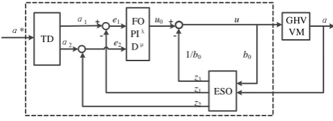
The ADRC method carries over the essence of the classical PID method and assimilates characteristics of the modern control theory. The traditional ADRC method consists of a tracking-differentiator (TD), a nonlinear state error feedback control law (NLSEF) and an extended state observer (ESO). The TD can coordinate the contradiction between rapidity and overshoot, the ESO can regard all disturbances as “unknown disturbances” [25, 26]. Compared with the traditional ADRC method, the FOPIλDμ ADRC method results in a FOPIλDμ controller instead of the NLSEF.A new nonlinear FOPIλDμ ADRC method is proposed and adopted to hypersonic vehicle control problem, the structure diagram is shown in Fig. 3. The structure diagram of the hypersonic vehicle VM FOPIλDμ ADRC method is shown in Fig. 3.

TD

FO PIλ Dμ

ESO

GHV VM

α*

α1 + +

-

-e1

z1

z3

u0 u

b0

1/b0

α

z2

e2 α2

Fig. 3: The structure diagram of the VM FOPIλDμ ADRC method for hypersonic vehicle

In Fig. 3, the desired attack angle α* _{is the input signal, the}

attack angle α is the output signal. TD, FOPIλDμ and ESO inside dashed line frame are the proposed controllers. The controlled object GHV VM is the vertical model of a hypersonic vehicle. α1 and α2 are the tracking signal of α* and

derivative signal of α1 from the TD, respectively. z1, z2 and z3

[image:2.595.313.554.569.657.2]

angle and unknown disturbances obtained from ESO, respectively. u0 is the ideal control variable and u is the

actual control variable.

The TD discrete form can be described by the following equations:

     

   





   



 



1 1 2

2 *

2 2 1 2

1

1 2

  

    

  

     

k k h k

k k h r k k r k (2)

where ₁

 

k and ₁



k1



denote estimated attack angle value of current time and next time, respectively, ₂

 

k and





2 1

 k are derivatives of ₁

 

k and ₁



k1



, respectively, r and h represent speed factor and filtering factor, respectively. The larger r values, the shorter the transition processes, the faster the response. The larger h values, the better for the noise filtering.

The FOPIλDμ equation is shown as follows:

 

 

_{ }

i

c p d

U s K

G s K K s

E s s

 

    (3)

Where  and  are restricted to0 , 1. The FOPIλDμ

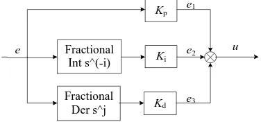
controller increases two degrees of freedom variables  and, thus making the control affect more precisely and stable. The structure diagram of the FOPIλDμ controller is shown in Fig. 4.

e

Kp

Fractional Int s^(-i)

Fractional Der s^j

e1

e2

e3 u Ki

[image:3.595.315.543.180.263.2]

Kd

Fig. 4: The structure diagram of the FOPIλDμ controller

In Fig. 4, e and u represent the error and control variable, respectively, e passes through Kp, FO integral method and

FO derivative method to get e1, e2 and e3, respectively.

The ESO in Fig. 3 is a third-order system and the extended state observer can be described by the following equation:

 

 

10 1

1 2 01 10

1 2

2 3 02 10 10 0

1 4

3 03 10 10

e

z

z

z

e

z

z

e

sign e

b u

z

e

sign e









 



  



  







 



(4)

where β01, β02 and β03 are adjustable parameters with

different values, which can affect the effect of signal observed, z1 and z2 are the estimated attack angle α and

estimated derivative signal of attack angle α, respectively, z3

is the estimated “unknown disturbances” of GHV VM and b0 is to affect the compensation of unknown disturbances.

With appropriate values of β01, β02 and β03, the ESO can have

good effect.

The LADRC method and the FOPIλDμ ADRC method are almost the same, except for the ESO method. The ESO of the FOPIλDμ ADRC method is nonlinear, while the ESO of the LADRC method is linear (LESO), which can be shown as follows:

10 1

1 2 01 10

2 3 02 10 0

3 03 10

e z

z z e

z z e b u

z e









  

   

   

    

(5)

Where meanings of variables are the same as those in Equation 4.

Therefore, the structure diagram of a hypersonic vehicle VM LADRC method is shown in Fig. 5.

TD

FO PIλ

Dμ

LESO

GHV VM

α*

α1 + +

-

-e1

z1

z3

u0 u

b0

1/b0

α

z2

e2

α2

Fig. 5: The structure diagram of the hypersonic vehicle VM LADRC method

In Fig. 5, the LESO is different from the ESO in Fig. 3 and the other parts are the same, and the meanings of variables are the same as those in Fig. 3. The ADRC method and the LADRC method both have more tuning parameters than the traditional PID method, while the appropriate controller parameters depend on the experiences of experts. Sometime, the number of the ADRC method parameters can be reduced to one or two [16, 20]. To compare the traditional ADRC method and the LADRC method clearly, this paper does not reduce parameters.

3.2 Analysis of FOPIλDμ ADRC method

We have analyzed the stability of the second-order ESO and the FOPIλDμ ADRC method [28]. The stability analysis of LESO and the FOPIλDμ LADRC method is the same.

3.2.1 The stability analysis of LESO

The pitch channel equation (1) can be written as follows:

1 2 2 ( ) 0

 

   

 _{ }

 f b u

(6)

Suppose the first-order derivative of f( ) exists and is bounded and define₃f( ), ( ) f t_w f( ) , (6) can be extended to (7).The LESO for (6) is (8).

1 2 2 3 0 3 ( )

 

 

    

 _ _



b u f

(7)

1 1 1

1 2 01 1

2 3 02 1 0

3 03 1 

         

   

    

e z

z z e

z z e b u

z e

(8)

Define e1 z1 1,e2z22,e3z33, from (7) and (8),

[image:3.595.74.262.360.448.2]

1 2 01 1

2 3 02 1

3 03 1 ( )

               w

e e e

e e e

e e f t

(9)

01

02

03

1 0 0

0 1 , 0 , ( )

0 0 1

       _{   }   _{ }  _  _           _{   }  w e Ae Bu

A B u f t

(10)

3 2

01 02 03

1

1 01

2 3 2

01 02 03

3 2

01 02

3 2

01 02 03

( ) ( ) ( ) ( ) ( ) ( ) ( ) ( ) ( ) ( )                          _{ }    _{   }   _{    }      _{  }     _{  }    W sf

s s s

E s

s s f

E s sI A BF s

s s s

E s

s s s f

s s s

(11)

The characteristic equation of (9) is:

3 2

01 02 03 0

  

   

s s s (12)

When

 

01 02



03,the LESO is stable. When f( ) is step

function or ramp function, LESO is able to track  1, 2, 3.

When f( ) _{is acceleration function, LESO is not able to}

track the desired signal.

3.2.2 The stability analysis of FOPIλDμ LADRC method

From Fig 5. , u₀and u can be shown as

*

0 1 1 1 1

*

2 2 2 2

3 0 0 ( )( ) ( )( )              _{   }       u p i d

u p i d

u K K s K s z

K K s K s z

z u u

b

(13)

*

1 1 1 1

*

2 2 2 21

1 2

2 3 3 0 ( )( )

( ( )( ))             _{  }            u p i d

u p i d

K K s K s z

s z

K b

K s K z

Let * *

1 0 , 0

        ,

*

1 1 1 1

* 2 3 2 2 0 2 (( )( ) ( )( ))                           u p i d

u p i d

K K s K s e

K K s K s e

e b (14) 2 0 2 0 0 0 0 2

01 02 1 1 1 0 01 2 2 2

3 3 2

01 02 03 2 2 2 1 1 1

*

1 1 1 2 2 2

2 ( ) ( ) ( )( ) ( ) ( ) ( )) ( ( ) ( )) (                                                   u u

p i d p i d

u u

p i d p i d

u u

p i d p i d b s

s sb b

b b s

s s s K K s K s b s s K K s K s

s s s K K s K s K K s K s

K K s K s K K s K

s

s sb₀( ₂ ₂  ₂ u) ₀( ₁ ₁  ₁ u)

p i d b p i d K K s K s K K s K s

(15)

1 2 2

01 02 1 1 1 0 01 2 2 2

* 3 3 2 01 0 2 0 0

02 03 2 2 2 1 1 1

*

2 2 2 2 2 0 ( ) ( ) ( )( ) ( ) ( ) ( )) ( (                                                           u u

p i d p i d

u u u

p i d p i d

p i d b

s b s b

s

s s s s K s K K s b s s K s K K s

s s s K s

s

K K s K s K K s

K s K K

b s ) 0( 1 1 1 )

  

 _{  } 

u u

p i d s b K s K K s

(16)

So the characteristic equation of (14) is:

2 2 2 0 1 1

2

0 ( ) ( 1 ) 0

  

  

 _{  } u _{  } u _

p i d p i d

s b s K s K K s b K s K K s (17)

Therefore, when parameters Kp1,Ki1,Kd1,Kp2,Ki2,Kd2 can

make all roots of characteristic equation (11) are on the left half-plane, the FOPIλDμ LADRC controller for hypersonic vehicles is stable.

4

Comparative simulation of FOPIλDμ ADRC

and FOPI

λ

D

μ

LADRC

Taking the longitudinal model of hypersonic vehicle as an example, the three modules of the auto disturbance rejection structure are tracking the differential device, the fractional order PID and the linear extended state observer. In order to compare and analyze the characteristics of the linear active disturbance rejection controller, the same structure of the active disturbance rejection controller is simulated, which is followed by the tracking controller, the fractional order PID and the extended state observer.

4.1 Comparative simulation of normal operating conditions

The angle of attack of the control system is a continuous square wave signal with amplitude of 10 degrees. The simulation results are shown in Fig. 6.

0 5 10 15

-5 0 5 10 15 20

(a) Time / s

a lp h a / d e g Input Nonlinear Linear

0 0.2 0.4 0.6 0.8 1 1.2 1.4 1.6 1.8 2

4 6 8 10 12

(b) Time / s

Fig. 6: Comparison of ADRC method and LADRC method without disturbances. (a) Comparison under disturbances; (b) Partial

enlarged view of (a)

In Fig. 6, the ‘Input’ represents the continuous square wave signal; ‘Nonlinear’ is a nonlinear active disturbance rejection controller. ‘Linear’ is a linear active disturbance rejection controller. Two control structures can make the output of the attack angle of attack fast tracking input signal, with a very small steady-state error and overshoot. The adjustment time of linear structure and nonlinear structure is 0.322s and 0.296s. Under the condition of no external disturbance, the control effect of the nonlinear active disturbance rejection control structure is better than that of the linear active disturbance rejection controller.

4.2 Electronic Image Files (Optional)

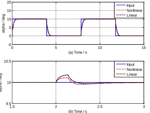
To show the anti-disturbance ability of the two controllers, the input signal is still a continuous wave signal with amplitude of 10 degrees. When the input signal is 2S and 7S, the interference signal is added. The interference signal amplitude is 90, and the duration is 140ms. The disturbance can be seen as an impact of the wind. The simulation results are shown in Fig. 7.

0 5 10 15

-5 0 5 10 15 20

(a) Time / s

a

lp

h

a

/

d

e

g

1.5 2 2.5 3

9.5 10 10.5

(b) Time / s

a

lp

h

a

/

d

e

g

Input Nonlinear Linear

[image:5.595.57.301.348.531.2]

Input Nonlinear Linear

Fig. 7: Comparison of ADRC method and LADRC method under disturbances. (a) Comparison under disturbances; (b) Partial enlarged view

of (a)

In Fig. 7, the meaning of each signal is the same as that of fig. 6.In Fig. 7(a), the two methods can track the reference signal rapidly. Two control structures are able to effectively track the input attack angle signal. In Fig. 7(b), the responses of ADRC method and LADRC method both have less than two percent changes lasting less than 1 s at 2 s, when subjected to external disturbance. But, the response of ADRC method with respect to the disturbance is more stable. Therefore, for hypersonic vehicle vertical model, the nonlinear controller demonstrates nominal better anti-disturbance ability and stronger robustness than the linear controller in some degree.

5

Conclusions

In this paper, by combining FOPIλDμ controller and the traditional ADRC method (TD, NLSEF and ESO), a FOPIλDμ ADRC controller is designed for hypersonic

vehicles. By replacing ESO with LESO, we obtain the FOPIλDμ LADRC controller. Then the differences of the FOPIλDμ ADRC method and FOPIλDμ LADRC are firstly clarified and analyzed. The stability of LESO and FOPIλDμ LADRC controller for hypersonic vehicle vertical model is analyzed. The experiment results show that the FOPIλDμ ADRC method performs better than the FOPIλDμ LADRC method.

References

[1] D. Cheng, Controllability of switched bilinear systems, IEEE Trans. on Automatic Control, 50(4): 511–515, 2005. [2] H. Poor, An Introduction to Signal Detection and Estimation.

New York: Springer-Verlag, 1985, chapter 4.

[3] B. Smith, An approach to graphs of linear forms, accepted. [4] D. Cheng, On logic-based intelligent systems, in Proceedings

of 5th International Conference on Control and Automation, 2005: 71–75.

[5] D. Cheng, R. Ortega, and E. Panteley, On port controlled hamiltonian systems, in Advanced Robust and Adaptive Control — Theory and Applications, D. Cheng, Y. Sun, T. Shen, and H. Ohmori, Eds. Beijing: Tsinghua University Press, 2005: 3–16.

[1] Gao G., Observer-Based Fault-Tolerant Control for an Air-Breathing Hypersonic Vehicle Model, Nonlinear Dynamics, 76(1): 409-430, 2014.

[2] Jiang B., Robust Fault-Tolerant Tracking Control for a Near-Space Vehicle Using a Sliding Mode Approach, System and Control Engineering, 225(8):1-12, 2011.

[3] Liu Z, Immersion and Invariance-Based Output Feedback Control of Air-Breathing Hypersonic Vehicles, IEEE Transactions on Automation Science & Engineering, 2015:1-9.

[4] Wiese D.P., Adaptive Output Feedback Based on Closed-Loop Reference Models for Hypersonic Vehicles, Journal of Guidance, Control, and Dynamics, 2015: 1-12. [5] Sun H. F., New Tracking-Control Strategy for Airbreathing

Hypersonic Vehicles, Journal of Guidance, Control, and Dynamics, 36(3): 846-859, 2013.

[6] Cai G. H., Flight control system design for hypersonic reentry vehicle based on LFT-LPV method, Proc IMechE, Part G: J Aerospace Engineering, 228(7):1130-1140, 2014.

[7] An H, Approximate Back-Stepping Fault-Tolerant Control of the Flexible Air-Breathing Hypersonic Vehicles, IEEE/ASME Transactions on Mechatronics, 2015:1-11.

[8] Li S. H., Composite Controller Design for an Air Breathing Hypersonic Vehicle, Proc IMechE, Part I: J Systems and Control Engineering, 226(5): 651-664, 2012.

[9] Duan H. B. and Li P., Progress in Control Approaches for Hypersonic Vehicle, Science China Technological Sciences, 55(10):2970-2965, 2012.

[10]Han J. Q., From the PID Technology to "Auto-Disturbance Rejection Control Technology, Control Engineering of China, 9(3):13-18, 2002.

[11]Guo B Z, Active disturbance rejection control approach to output feedback stabilization of a class of uncertain nonlinear systems subject to stochastic disturbance, IEEE Transactions on Automatic Control, 2015.

[12]Shi X. X., Motion Control of a Novel 6-degree-of-Freedom Parallel Platform Based on Modified Active Disturbance Rejection Controller, Proc IMechE, Part I: J Systems and Control Engineering, 228(2):87-96, 2014.

[13]Zhao L, Active Disturbance Rejection Position Control for a Magnetic Rodless Pneumatic Cylinder, IEEE Transactions on Industrial Electronics, 62(9):1-1, 2015.

Disturbance Rejection Controller, Proc IMechE, Part I: J Systems and Control Engineering, 226(5):606-614,2011. [15]Sun G, Neural Active Disturbance Rejection Output Control

of Multimotor Servomechanism, IEEE Transactions on Control Systems Technology, 23(2):746-753, 2015.

[16]Peng C, Mismatched Disturbance Rejection Control for Voltage-Controlled Active Magnetic Bearing via State-Space Disturbance Observer, IEEE Transactions on Power Electronics, 30(5):2753-2762, 2015.

[17]Tang Y. M., Linear Active Disturbance Rejection-Based Load Frequency Control Concerning High Penetration of Wind Energy, Energy Conversion and Management, 95: 259-271, 2015.

[18]Tan W, Linear Active Disturbance Rejection Control_ Analysis and Tuning via IMC, IEEE Transactions on Industrial Electronics, 2015:1-9.

[19]Ramírez-Neria M., Linear Active Disturbance Rejection Control of Underactuated Systems: the Case of the Furuta Pendulum, ISA Transactions, 53(4): 920-928, 2014. [20]Sira-Ramírez H., Linear Observer-Based Active Disturbance

Rejection Control of the Omnidirectional Mobile Robot, Asian Journal of Control, 15(1): 51-63, 2013.

[21]Zheng Q. L., Active Disturbance Rejection Control for Piezoelectric Beam, Asian Journal of Control. 16(6): 1612-1622, 2014.

[22]Shaughnessy J. D., Hypersonic Vehicle Simulation Model: Winged-Cone Configuration, NASA Langley Research Center, 1990.

[23]Shahriar K., Development of An Aerodynamic Database for A Generic Hypersonic Air Vehicle, AIAA Guidance, Navigation, and Control Conference and Exhibit, 2005:2005-6257. [24]Song J, Nonlinear Fractional Order

Proportion-Integral-Derivative Active Disturbance Rejection Control Method Design for Hypersonic Vehicle Attitude Control, Acta Astronautica, 111:160-169, 2015.

[25]Han J. Q., From PID to Active Disturbance Rejection Control, IEEE Transactions on Industrial Electronics, 56(3): 900-906, 2009.