City, University of London Institutional Repository
Citation:
Kontsevich, L.L. & Tyler, C. W. (2013). A simpler structure for local spatial channels revealed by sustained perifoveal stimuli. Journal of Vision, 13(1), p. 22. doi: 10.1167/13.1.22This is the accepted version of the paper.
This version of the publication may differ from the final published
version.
Permanent repository link:
http://openaccess.city.ac.uk/5878/Link to published version:
http://dx.doi.org/10.1167/13.1.22Copyright and reuse: City Research Online aims to make research
outputs of City, University of London available to a wider audience.
Copyright and Moral Rights remain with the author(s) and/or copyright
holders. URLs from City Research Online may be freely distributed and
linked to.
1. Author: This article has been lightly edited for grammar, style, and usage. Please compare against your original document and make changes on these pages. Please limit your corrections to substantive changes that affect meaning. If no change is required in response to a question, please write‘‘OK as set’’in the margin. Copy editor 2. Author: Please provide websites and/or emails for all authors if available. Copy editor
3. Author: Please provide the corresponding author’s mailing address. Copy editor
4. Author: Make sure that ALL funding/financial support is listed in the Acknowledgments section. Copy editor 5. Author: Please note that Wilson et al. (1985) does not have a matching reference. Is the 1983 reference intended?
Copy editor
6. Author: Please note that Kersten (1984) does not have a matching reference. Copy editor
7. Author: Please note that Wilson et al. (1985) does not have a matching reference. Is the 1983 reference intended? Copy editor
8. Author: Please update Kontsevich & Tyler (in preparation) if possible. Copy editor
9. Author: Please note that Foley & Legge (1975) does not have a matching reference. Copy editor
10. Author: Please verify that the sentence beginning‘‘A compromise for low’’is correct as edited. Copy editor 11. Author: Please define all equation terms following the equations if they have not been previously defined. Copy
editor
12. Author: Please note that Wilson et al. (1987) does not have a matching reference. Copy editor 13. Author: In the sentence following Equation 3, shouldT¼3sbeT¼3 s? Copy editor
14. Author: Please note that Daniel & Whitteridge (1961) does not have a matching reference. Copy editor 15. Author: Please provide acknowledgments information. Copy editor
A simpler structure for local spatial channels identified
with sustained stimuli in the visual periphery
Leonid L. Kontsevich
Smith-Kettlewell Eye Research Institute,San Francisco, CA, USA$
Christopher W. Tyler
Smith-Kettlewell Eye Research Institute,San Francisco, CA, USAA
?1 new evaluation of the local structure of spatial channels with local stimuli in peripheral retina employs the masking sensitivity approach to minimize analytic assumptions.
?2 The stimuli were designed to address the range of channel tunings of the predominantly sustained response system in the near periphery.
?3 Under these conditions, the range of identifiable channels spanned a narrow range of spatial frequencies, from roughly 2–8 cpd at 28 eccentricity to 1–4 cpd at 88 eccentricity. The analysis showed that there are no sustained channels tuned below 2 cpd for the central visual field. This two-octave range of channel tuning is much narrower than is conventionally assumed. For local sustained stimuli, human peripheral spatial processing therefore appears to be based on a simpler channel structure than is often supposed.
?4
Keywords: cortical scaling, contrast sensitivity, masking, periphery, spatial vision
Citation: Kontsevich, L. L., & Tyler, C. W. (2013). A simpler structure for local spatial channels identified with sustained stimuli in the visual periphery.Journal of Vision, 13(1):X, 1–11,http://www.journalofvision.org/content/13/1/XX, doi:10.1167/ 13.1.XX.
Introduction
One of the major issues of modern psychophysics used to be the spatial channel structure across the retina. Despite many attempts to estimate this structure over the past three decades, only one study focused on the issue of the spatial frequency tuning for local retinal regions (Swanson & Wilson,1985). All other studies to our knowledge used stimuli that covered considerably inhomogeneous retinal and cortical areas relative to the fovea-centered scaling of neural processing. Throwing multiple channels from different locations into one basket makes the results hard to interpret. Even the 1.58
foveal stimulus of Blakemore and Campbell (1969), for example, may be expected to have stimulated about 500 cortical hypercolumns (Tyler & Apkarian, 1982; Levi, Klein, & Aitsebaomo,1985) with an eccentricity scaling of about 3 to 1.
The most local study of channel structure to date, therefore, appears to have been that of Swanson and
Wilson (1985), who used an oblique masking paradigm
at 88 eccentricity to determine the masking functions for sixth-derivative-of-Gaussian test stimuli. They concluded that the six-mechanism model of Wilson, McFarlane, & Phillips (1983) construed for the central retina explains the masking results for the periphery if the channel mechanisms are scaled to lower frequencies by a factor of 2. Although this was a relatively
successful curve-fitting exercise, no attempt was made to evaluate the adequacy of alternative models, such as the four-channel model of Wilson and Bergen (1979) or the two-channel model of Tyler and Apkarian (1982). Moreover, the Swanson and Wilson (1985) model fits to the eccentric data were inaccurate by as much as one third of the peak masking amplitude (where the measurement noise appeared to be about one tenth of peak masking). Although the model accounted for 92% of the masking variance, the deviations appeared consistent enough to warrant further examination of the issue of channel structure. (For example, 6 of their 10 curves showed adjacent points that deviated in the same direction from the model predictions by more than one standard deviation.)
A further problem with the Wilson et al. (1985) model is the extended inferential sequence required to derive
the channel structure from the masking data. The ?5
analysis required measurement of the contrast depen-dence of the masking behavior, estimation of the channel combination rule, and iterative optimization of the multiple-channel model to the data. A particular problem was the assumption of the high value of 4 for the Minkowski summation exponent among channel outputs, justified on the basis of the steepness of the unmasked psychometric function (Williams & Wilson,
1983). Under masking conditions, detection of the test is essentially a suprathreshold discrimination task in which the psychometric function is likely to have a shallow Journal of Vision(2013) 13(1):0, 1–11 http://www.journalofvision.org/content/13/1/0 1
unity slope (Wilson, 1980; Kersten, 1984; Legge, Kersten, & Burgess, 1987), violating the assumption leading to a steep combination rule.
?6 The model fits to the
peripheral masking data cannot therefore be regarded as a definitive measure of local channel structure.
Another problem with the Wilson et al. (1985) study was that a key requirement was the fitting of the contrast sensitivity function, which was treated as a direct combination of contrast sensitivities of the underlying channels.
?7 The binocular contrast
summa-tion study carried out by Legge (1984), however,
indicates that an accelerating contrast nonlinearity, which manifests itself in the ‘‘dipper’’ in the contrast discrimination function, precedes both the binocular summation site and the cortical mechanisms responsi-ble for spatial frequency selectivity. Our own study (Kontsevich & Tyler, in preparation) revisited the binocular contrast summation issue and fully con-firmed the notion of an early accelerating nonlinearity for contrast.
?8 We show that such a nonlinearity
inevitably leads to flattening of the contrast sensitivity function. The tails of the flattened contrast sensitivity function cannot be matched by the tails of the individual channels, and therefore the failure to take such a flattening into account should drive the model to imply a wider range of spatial frequency channels than is actually present.
We therefore re-evaluated the properties of local spatial tuning with an enhanced psychophysical para-digm that measures the channel structure directly without the need for any computational modeling. The results provide a substantially different picture of peripheral channel structure than that of Swanson and Wilson (1985), with very few interpretive assumptions. We show that the required assumptions are substantially supported by the available data where tests are feasible.
Rationale
To take less model-based approach to assessment of the local channel structure, we adopted the masking sensitivity paradigm, introduced by Stiles (1939) as the
field sensitivity paradigm. In our version of this approach, the test stimulus is set at a fixed level above its contrast detection threshold (2 to 3 times higher) and the masking strength required to return the test to the threshold is determined as a function of mask spatial frequency. Channel masking theory predicts (see
Appendixfor detail) that when the test is detected by a single channel, the resulting masking sensitivity curve accurately reflects the channel tuning function, and possible nonlinearities in channel transduction have no effects on the result. This feature makes the masking sensitivity paradigm unique among other masking
paradigms (e.g., Blakemore & Campbell, 1969; Foley & Legge, 1975; Wilson et al., 1983). ?9
When a test is ‘‘seen’’ by several channels, the masking curve is a result of the interaction of all channels involved. Estimation of this interaction inevitably requires computational modeling, whatever masking method is chosen (including the masking sensitivity paradigm). In the present study we mini-mized the application of such a modeling because the additional assumptions that are inevitably required weaken the results. To focus on the most direct measurements, we limited our task to assessing only the extreme channels, those that determine the upper and lower bounds of the contrast sensitivity function in spatial frequency domain. It is safe to assume that a test located on the outer tail of such a channel could be detected only by this channel without interference from the others. Our goal was therefore to measure the masking sensitivity curve existing under these condi-tions, which should reflect the tuning function of the upper and lower channels alone. The fine channel structure between the extreme channels was therefore beyond the scope of the study.
One of the primary goals of the present study was to assess the spatial channel structure locally. The rationale was straightforward. Since the spatial resolution of the visual mechanisms rapidly degrades with eccentricity (Robson & Graham,1981), measurement of the channel structure for an extended central area represents a meaningless undertaking because the channels of different spatial scale at different eccentricities operate in one big pool. The channel range in this case would depend more on the area stimulated by the test stimulus than the channel range specific for a particular location in the visual field and, therefore, would not tell much about the channels. Our approach was similar to that of Swanson and Wilson (1985), who assessed the channel structure in a local region of the peripheral visual field small enough to be essentially homogeneous.
To test as uniform a part of the visual field as possible, the size of the test stimulus should be small relative to its eccentricity. On the other hand, some degree of selectivity to spatial frequency should be maintained. It is easy to find the compromise condi-tions for the high spatial frequency test because multiple periods will fit into a small patch and Gabor stimuli can be used. A compromise for low spatial frequencies is harder to achieve but was solved as
explained in the following section. ?10
Stimulus Justification
have multiple positive and negative lobes, in order to achieve narrowband specificity. Unlike the test stimuli used in most previous studies, Gaussian bars are lowpass rather than narrowband stimuli. This property, however, does not mean that the visual channels are not selective to Gaussian bars of a certain width. Consider a neuron with a classical cortical receptive field that has an elongated excitatory area counterbal-anced by two inhibitory areas, one on each side. When the test is a very narrow Gaussian bar aligned within the excitatory area, the response of the neuron will be quite small because only a small part of the excitatory area is stimulated. Conversely, if the stimulus bar is very wide, the response will again be small because the test stimulates both the excitatory and inhibitory areas, which cancel each other’s responses. The optimal stimulus is the bar whose width is close to the width of the excitatory strip because this stimulus activates the full extent of the excitatory area and does not activate the inhibitory area. Thus, receptive fields with bandpass tuning for narrowband stimuli also have bandpass tuning to Gaussian bars.
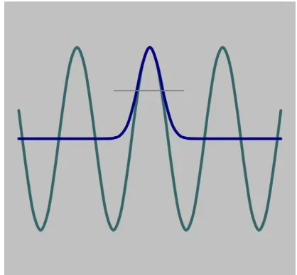
One problem with Gaussian bars, as with any local stimuli, is to relate the spatial and spatial frequency parameter of the bars because this relationship depends somewhat on the receptive-field profile (though varia-tion of this relavaria-tionship across different profiles is small). In the present study we compare the spatial profiles of Gaussian bar and the cosine grating in the peak area; the bars were assigned the spatial frequency of a grating that had the matching peak profile, as shown inFigure 1.
?11 Thus, the relationship between the
spatial parameter of the bar and the grating frequency was derived on the basis of equality of the second derivatives at the peak:
d2ex2=r2
dx2 ¼
d2cosð2pfxÞ
dx2 ð1Þ
which leads to the equality
f¼ ffiffiffi1
2
p
pr ð2aÞ
and, conversely,
r¼ ffiffiffi1
2
p
pf ð2bÞ
There are other ways to estimate the matching spatial frequency to the Gaussian bar; for instance, one can look for a spatial frequency that produces the maximum normalized response of a cosine or a plausible Gabor receptive field. These estimates differ from the one provided by Equation 2 by only a few percent, so we will stay withEquation 2assuming that it provides a good approximation for any underlying mechanism.
When the mask has low spatial frequency, its masking effect may not be uniform across space, i.e., different at the mask peaks, troughs, and in the transitional areas. Investigation of such a phase effect could constitute a study on its own. To avoid this complication we adopted the oblique masking paradigm (Wilson et al., 1987), which uses a mask with slightly different orientation than a test. Due to this orientation mismatch all phase ?12 relations are present in a small area and the task becomes effectively phase independent.
The last issue that requires careful consideration is the time course of the stimuli. The shape of the contrast sensitivity function is known to depend upon the temporal frequency of stimuli: being bandpass at low temporal frequency and low pass at medium-high
temporal frequencies (Robson, 1966). This transition
can be attributed to a sluggish surround of the receptive fields (Reid & Shapley, 2002). If this explanation is correct, a similar transition from bandpass to lowpass spatial frequency tuning function should take place for each individual receptive field; therefore, at higher temporal frequencies or in brief presentations, the channels may lose selectivity in the spatial frequency domain, which in turn would make it hard to take them apart in the low-spatial-frequency domain. To avoid this potential problem we decided to maintain the narrowest possible tuning of the channels studied by conducting the masking study with sustained presentation.
Methods
[image:5.666.368.577.88.282.2]The stimuli were presented in a dark room on two 14-in. Sony monitors controlled by visual attenuators Figure 1. Gaussian and cosine modulations with matched second derivatives at the peak. Widths of the profiles at half height (shown by a horizontal line) are also tightly matched.
(Institute for Sensory Research, Syracuse University) and the Video Toolbox software (Pelli & Zhang,1991; Brainard, 1997) running on an Apple G4 computer. The monitor resolution was set at 800 by 600 pixels with a frame rate of 100 Hz. Test and mask stimuli were presented on different monitors with the background luminance at 25 cd/m2. These images were combined by a half-transparent front-surface mirror, such that the visible contrast of the stimuli was half of that on the screen. All data in this study are specified in terms of the visible contrast of the combined image. The stimuli were presented to observer’s right eye at a distance of 136 cm, while the left eye was covered by an eye patch. The range of spatial frequency channels was evaluated at three eccentricities: 28, 48, and 88. For 28
and 48the fixation cross was located in the center of the screen and the test could appear randomly on either side, as shown inFigure 2. In this case a two-alternative forced-choice (2AFC) task was used: the observer had to say on which side the test was presented. In the case of the 88eccentricity condition, the screen was too small for such a bilateral presentation. In this condition the fixation was set beyond the edge of the screen and the mask and the maskþtest stimuli were shown at the screen center in the two-interval forced-choice (2IFC) procedure. Beginning of the 2IFC presentation inter-vals were indicated by brief (100 ms) sounds.
The mask was an oblique sinusoidal grating tilted by 108to the vertical and filled the whole screen. For the 28
and 48 eccentricity conditions it had a small blank field in the center, where the fixation cross was shown. The test stimulus, depending on whether the higher or lower channels were measured, had either an elliptical Gabor or elliptical Gaussian luminance profiles (Figure 2). Both test and mask were presented in synchrony with a raised cosine temporal profile with a 3-s epoch. The Gaussian profile had a fixed height and a width that
varied with eccentricity, as specified by the formula:
Lðx;y;tÞ ¼L0þL0ce
ðx6pÞ2 r2 þ
y2
ðd=4Þ2
1cos 2pt T
2
ð3Þ
whereL0is the background luminance,cis the contrast parameter,pis the test eccentricity on a given trial,ris the Gaussian width parameter computed based on
Equation 2bfrom the spatial frequencyfprobed by the Gaussian bar,dis the test eccentricity, andT¼3sis the presentation epoch.When the test had a Gabor profile, ?13 the envelope was vertically elongated by a factor of 2 and the cosine bars were vertical:
Lðx;y;tÞ ¼L0þL0ce
ðx6pÞ2 ðd=8Þ2 þ
y2
ðd=4Þ2
·cos2pfðxpÞ1cos
2pt T
2 : ð4Þ
A Gaussian test superimposed with a mask is illustrated on the left panel of Figure 2, while the right panel illustrates the Gabor test. It should be noted that this Gaussian test example is close to the widest employed in the experiments. To sample the visual field, the experiments were conducted with the test at three different eccentricities: 28, 48, and 88 to the right of fixation.
[image:6.666.90.581.552.733.2]An experiment consisted of a series of measurements varying mask spatial frequency for a fixed test stimulus. Each series began with a measurement of the test detection contrast with no mask present. Then, the test contrast was set at twice the detection threshold, and the mask threshold contrast was measured for sampled spatial frequency values of the mask with half-octave step. Sometimes, probably because of observer fatigue, the detection threshold increased during an experimen-tal series to a level at which observer stopped reliably
seeing the test alone for extended periods of time. In such cases the whole routine was terminated and started over with a new measurement of the detection threshold. We encouraged observers to take frequent rests to avoid such problematic events.
All measurements were conducted with three-down/
one-up nonparametric adaptive method (Levitt,1971),
which converges at 75% correct. Every measurement was repeated at least three times, and the results were averaged. In cases in which the maximum contrast mask did not bring the test to threshold, we depicted the tuning function as if the mask contrast was 50% at that point (a maximum value, since two screens were mixed with half-transparent mirror) to express widest tuning function compatible with the failure to reach threshold. We did not employ a Bayesian adaptive method because there were no data on the value and stability of the psychometric slope in the masking sensitivity task. Also, the relatively high miss error level in this task would have dramatically reduced the efficacy of the adaptive methods. A potential compli-cation with the masking sensitivity paradigm might be the susceptibility of the masking sensitivity results to fluctuations in the contrast detection threshold, which are known to be dependent, for instance, on the time of day and the blood glucose level (Barlow, Khan, & Farell, 2003). To address this issue, we varied mask spatial frequency in both in ascending and descending order and averaged their masking sensitivities in logarithmic space. Such a procedure removes any directional bias on the shape of the masking sensitivity curves.
The experiments were conducted with one of the authors and two paid observers: all male, 14 to 44 years old, with normal vision without correction. Two of them were experienced observers who had participated in numerous psychophysical experiments; for the third it was the first psychophysical experiment. Two observers were na ¨ıve about the goal of the study, the other being the first author of the paper.
Results
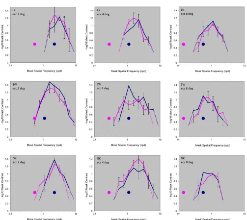
The experiment results for masking of low-frequency channels are shown inFigure 3. All masking sensitivity curves were measured with the elliptical Gaussian test stimuli. Colored dots in this figure depict the test effective spatial frequency (see Equation 2a) and the curve of the same color depicts the corresponding masking sensitivity function. The higher effective spatial frequency test was set at the point where the test contrast sensitivity was the highest. The lower effective spatial frequency was set to be separated from the highest one by two octaves (with one exception for
observer SW at 28 eccentricity). The graphs are shown on a double logarithmic scale. It is evident that the masking effects all show narrowband tuning functions peaking at 0.5–1 cpd for the 88eccentricity curves, at 1– 2 cpd for the 48 eccentricity curves and at 2–3 cpd for the 28 eccentricity curves.
The data show two characteristics critical for the interpretation of the channel structure underlying the detection performance. One is that, for the lower frequency test stimuli, the masking sensitivity curves peak at a frequency higher than the effective frequency of the tests. The other is that the tunings for the two tests were very similar in form and peak frequency, despite the test frequencies differing by two octaves (or by one octave in one case). In all cases, use of a test with the lower frequency produced a masking function entirely above the test frequency throughout its measurable range, which did not differ significantly (as discussed in following text) from the masking effect for the higher frequency test. The most parsimonious interpretation of these results is that performance is mediated by a single size-tuned channel at each eccentricity.
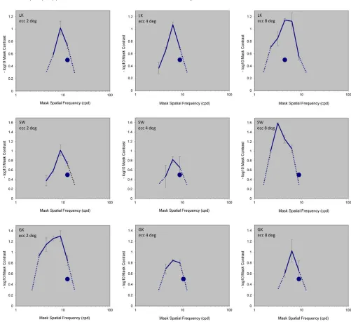
The corresponding tuning functions for the masking of high-frequency channels are compiled in Figure 4. The graphs are shown with the same conventions as in
Figure 3except that all masking sensitivity curves were measured with the narrowband Gabor test stimuli. The blue dots show the effective spatial frequency of the test stimuli. For each observer and condition it was set half an octave lower than the highest visible spatial frequency in the experimental setup (zero contrast mask, 50% contrast test) in order to allow room for the requisite contrast variation. These data show that the masking effect peaksbelowthe test frequency for all but one of the high-frequency conditions, where it coincides with the test frequency (subject LK at 88 eccentricity). This result suggests that the local highest frequency channel peaks at the frequencies somewhat below the maximum detectable spatial frequency at 100% con-trast.
Analysis
The results presented reveal a number of novel features of the spatial frequency channels. Let us start with the analysis of low-frequency range.
First and foremost, in each panel of Figure 3, the blue and magenta masking sensitivity curves closely overlap. Each blue curve was measured for the test whose spatial tuning was close to the spatial tuning of the masking sensitivity curve. For each magenta curve the spatial tuning of the test was about two octaves below the masking sensitivity curve tuning. These
results are inconsistent with the behavior expected for a continuous channel system, which should show mask-ing sensitivity peakmask-ing at each test frequency (or at least shifted by an equal amount from each test frequency). The only reasonable interpretation is that the joint masking sensitivity function for the two test frequencies represents the sensitivity of asinglechannel peaking at a frequency well above that of the higher test frequency. Moreover, this joint function implies that
there are no functional channels below the one defined at each eccentricity. The broader implication is that there is not a continuous set of spatially tuned channels at each eccentricity but a limited range that begins above 1 cpd for all eccentricities tested.
[image:8.666.82.585.75.524.2]In terms of bandwidth there was no obvious change in the shapes of the functions with eccentricity. Quantitative evaluation gave an average bandwidth of 1.7060.08 octaves for the tuning of the lowest channel Figure 3. Masking sensitivity curves for three observers for Gaussian test stimuli that probed low frequency channels, at 88, 48, and 28
(Figure 3), and 1.0760.12 for the highest one (Figure 4).
Comparison of the masking sensitivity curves across eccentricity reveals that the spatial tuning of the lowest channel gradually shifts to lower spatial frequencies as eccentricity increases. This shift is illustrated in the left panel ofFigure 5 for observer LK.
Similarly the specification of the lowest channel, the experiments with the high-frequency test reveal the channel tuned to the highest frequency. The right panel ofFigure 5illustrates that the tuning frequency for this channel also tends to shift to lower spatial frequencies as eccentricity increases.
In the data shown in Figure 4, the mask with a
[image:9.666.81.582.74.533.2]spatial frequency half an octave higher than the test spatial frequency usually had a measurable masking effect. On the other hand, as described earlier, the frequency for the high-frequency test was chosen half an octavelowerthan the spatial frequency threshold for 100% contrast. These two statements do not imply that we found a measurable masking effect for the mask that an observer could not see. In fact, the mask in our measurements was always visible because it occupied the whole screen and its detection threshold was lower than that for local test stimulus due to spatial summation (Kelly, 1975; Robson & Graham, 1981; Rovamo, Luntinen, & Nasanen,1993).
Figure 4. Masking sensitivity curves for Gabor test stimuli that probed high frequency channels, in the same format asFigure 3. The blue dots depict spatial frequency of the test, which was set half an octave below the maximum resolvable effective spatial frequency for the stimulus at each eccentricity for each observer.
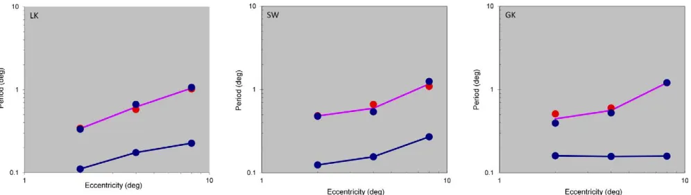
Having revealed the extreme channel locations, the channel range at different eccentricities can be ana-lyzed. We estimated the channel tuning frequency as the center of gravity of the tuning function on the logarithmic spatial frequency axis, when the masking sensitivity was expressed in linear units (1/c instead of
log(c) as inFigures 3to5. The results are presented in
[image:10.666.153.516.87.237.2]Figure 6for all three observers on a double logarithmic scale (chosen because it translates constant ratios into constant distances, which are much easier to grasp visually): the horizontal axis shows the eccentricity and the vertical axis shows the period of the channel tuning frequency in units of degrees. The channel tuning at low frequencies was estimated at both measured test sizes; the colors of points corresponds to those in
Figure 3.
To validate the earlier claim that channel tuning at low frequencies did not significantly differ between both measured test sizes, we ran Monte Carlo simulations for the peak estimate after adding normally distributed jitter to each measured data point with the
standard deviation estimated in the experiment and
depicted by error bars in Figure 3. As a result, we
computed a standard deviation of the peak estimate for every condition. For all observers and eccentricities the difference between the peak estimates for two peak sizes was within the 2 sigma range.
The distance between the red and green curves varies by a factor of about 3–6 across eccentricities and observers. This observation suggests that the local channel structure has a limited range of about a factor of 4 at each eccentricity.
Discussion
The described experiments indicate that the spatial frequency range of local channels responsible for contrast detection is narrower than the spatial cy range of contrast sensitivity function. The frequen-cies outside the channel range, as our experiments Figure 5. The masking sensitivity curves measured for (left panel) the lowest frequency test and (right panel) the highest frequency test. In both cases the curve tuning shifts to lower frequencies (leftward) as the eccentricity increases.
[image:10.666.86.584.554.695.2]indicate, are detected due to a residual signal from the lowest and the highest frequency channels.
The analysis of Figure 6 shows that, on average
across observers, the distance between the upper and lower spatial frequency peaks is about a factor of 4 (two octaves) across eccentricity. This observation suggests that the local channel structure is relatively invariant across eccentricity; the only thing that varies is the scale of the whole set of channels. In other words, the channel range remains about the same at each location in the visual field and is only two octaves in width. In terms of preferred stimulus widths, the range goes from about 1/20 to 1/5 of the eccentricity of stimulation. We propose that the explanation for these results is that the receptive field populations are uniform in cortical units (millimeters) and their increase in retinal size with eccentricity is solely due to cortical magnification (Daniel & Whitteridge, 1961; Virsu & Rovamo, 1979; Tootell Silverman, Switkes, & De Valois, 1981; Tyler & Apkarian, 1982; Schira, Wade, & Tyler, 2007; Schira, Tyler, Spehar, & Breakspear,
2010).
?14 This would be very simple and elegant structure underlying cortical visual processing.
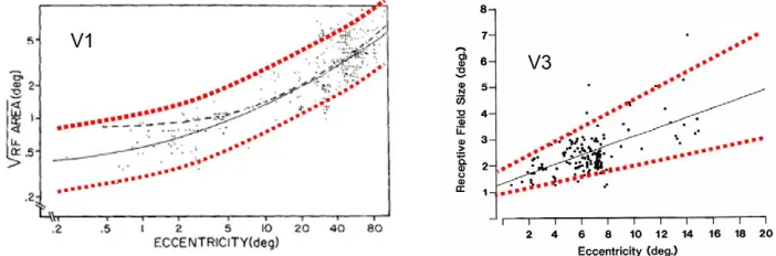
This idea is consistent with the results of single unit recording conducted on visual area V1 in the Cebus monkey (Gattass, Sousa, & Rosa, 1987) and on visual area V3 in the macaque monkey (Felleman & Van Essen,1987), which are reproduced inFigure 7. In both cases the range of the cortical filter sizes in a particular location fell within about a two-octave range across the full range of eccentricities, even though the mean size varied by a factor of about 10. These results do not seem to have made much impact on the channel modelers of the past several decades, who typically assume a full range of channel sizes without taking eccentricity into account.
The implication that the channels cover only a narrow two-octave range of spatial frequencies at each eccentricity raises an interesting question: how can observers see the gratings with spatial frequencies below the lowest and above the highest frequency channels? If the channels cover a limited range of spatial frequencies, responses outside the range of the peak channel sensitivities must necessarily be corre-spondingly attenuated, as is indeed the case for measurements of local sensitivity with eccentricity
(e.g., Virsu & Rovamo, 1979). We suggest that
observers see these out-of-range gratings not by the channels but rather through the channels, in the sense that the visual system compares the attenuated local channel responses across the visual directions and integrates these local responses into an extended grating percept. In terms of receptive fields, this means that the array of local receptive fields transmits the signal to provide a sinusoidal response profile across the cortex, and this profile is then processed by subsequent mechanisms that do not have a tuned channel structure (such as an attentional comparator; Intriligator & Cavanagh, 2001) or attentional shroud (Tyler & Kontsevich, 1999). This idea of post-processing integration across local mechanisms for low-frequency gratings was originally suggested by Stromeyer, Klein, Dawson, and Spillmann (1982). It is consistent with the concept of analysis by second-order mechanisms beyond the level of the primary processing channels (He & Nakayama, 1994; Landy & Graham,
[image:11.666.157.508.543.659.2]2004), although those analyses tend to emphasize the local aspects of this second-order processing in terms of the receptive-field selectivity of individual second-order neurons, and do not comment on its potential role in processing long-range aspects of the processing of low-frequency first-order stimuli.
Figure 7. The scatter plot on the left panel is a double-logarithmic plot of the receptive field sizes in the Cebus monkey area V1 from Gattass et al. (1987) and the scatter plot in the right panel shows the receptive field sizes in the macaque area V3 from Felleman and Van Essen (1987) in linear coordinates (both figures are reproduced with authors’ permission). In the left panel, the red dotted curves delineate the two-octave range for the receptive field size centered at its mean, which is depicted by the solid black curve (their dashed curve is not relevant to our point). Notice that the most of the V1 data fall within a61-octave range from the mean, which is consistent with our observations and does not support the concept of an extended range of spatial-frequency channels at any eccentricity. The V3 data on the right panel fall within an even narrower,61-octave range (red dotted lines), again supporting the concept of a narrow range of spatial channels at any eccentricity. The solid black line is the best-fit linear slope to the data.
Although, Stromeyer et al. (1982) suggested the idea of integration across local mechanisms for low-fre-quency gratings, we are not aware of similar explana-tion for seeing gratings of very high frequency. If the sampling density was matched to the peak tuning frequency of the receptive fields (e.g., with a spacing of a quarter of the cycle of the Gabor carrier frequency), it would provide oversampling for very low frequencies but, conversely, undersampling for much higher frequencies than the peak of the outermost channel. Such undersampling could account for the break-up of the perception of gratings into noisy irregular pieces at very high frequencies (Purkinje, 1819; Tyler & Na-kayama,1980).
Conclusions
We measured masking sensitivity curves with local test stimuli at several eccentricities to assess the structure of sustained spatial frequency channels across the visual field. At each eccentricity the masking behavior suggests that there is a lowest and highest spatial frequency channel and the difference between their frequencies is only about two octaves. The lack of channels outside this range accounts for the fall-off in sensitivities at both high and low spatial frequencies. We attribute a general shift in the tuning of the channels toward lower spatial frequency with eccen-tricity to cortical magnification and suggest that populations of cortical receptive fields have the same sizes across a given cortical area if measured in cortical units. To explain how observers see the gratings outside the channel range, we suggest that the visual system has a subsequent process that compares the channel outputs across visual directions.
Acknjovowledgments
?15
Commercial relationships: none.
Corresponding author: Leonid L Kontsevich. Email: [email protected].
Address: Envizio, Inc., Fremont, CA, USA.
References
Barlow, R., Khan, M., & Farell, B. (2003). Time of day and glucose modulate visual sensitivity [Abstract]. Journal of Vision, 3(9):356, 356a, http://www.
journalofvision.org/content/3/9/365, doi:10.1167/3. 9.365.
Blakemore, C., & Campbell, F. W. (1969). On the existence of neurons in the human visual system selectively sensitive to the orientation and size of retinal images.Journal of Physiology, 203, 237–260. Brainard, D. H. (1997). The Psychophysics Toolbox.
Spatial Vision, 10, 433–436.
Felleman, D. J., & Van Essen, D. C. (1987). Receptive field properties of neurons in area V3 of macaque
monkey extrastriate cortex. Journal of
Neurophys-iology, 57, 889–920.
Gattass, R., Sousa, A. P., & Rosa, M. G. (1987). Visual
topography of V1 in the Cebus monkey.Journal of
Comparative Neurology, 258, 529–548.
He, Z. J., & Nakayama, K. (1994). Perceiving textures: beyond filtering.Vision Research, 34, 151–162. Intriligator, J., & Cavanagh, P. (2001). The spatial
resolution of visual attention. Cognitive Psycholo-gy, 43, 171–216.
Kelly, D. H. (1975). How many bars make a grating? Vision Research, 15, 625–628.
Landy, M. S., & Graham, N. (2004). Visual perception of texture. In: L. M. Chalupa & J. S. Werner (Eds.), The visual neurosciences (pp. 1106–1118), Cam-bridge, MA: MIT Press.
Legge, G. E. (1984). Binocular contrast summation— II. Quadratic summation.Vision Research, 24, 385– 394.
Legge, G. E., Kersten, D., & Burgess, A. E. (1987).
Contrast discrimination in noise. Journal of the
Optical Society of America. A, Optics and Image Science, A4, 391–404.
Levi, D. M., Klein, S. A., & Aitsebaomo, A. P. (1985). Vernier acuity, crowding and cortical magnifica-tion. Vision Research, 25, 963–977.
Levitt, H. (1971). Transformed up-down methods in psychoacoustics. Journal of the Acoustical Society of America, 49, 467–477.
Pelli, D. G. (1997). The VideoToolbox software for visual psychophysics: transforming numbers into
movies.Spatial Vision, 10, 437–442. ?16
Pelli, D. G., & Zhang, L. (1991). Accurate control of
contrast on microcomputer displays. Vision
Re-search, 31, 1337–1350.
Purkinje, J. E. (1819). Beobachtungen und Versuch zur
Physiologie der Sinne. University of Prague:
Prague.
Robson, J. G. (1966). Spatial and temporal contrast sensitivity functions of the human visual system. Journal of the Optical Society of America, 56, 1141– 1142.
Robson, J. G., & Graham, N. (1981). Probability summation and regional variation in contrast sensitivity across the visual field. Vision Research, 21, 409–418.
Rovamo, J., Luntinen, O., & Nasanen, R. (1993). Modelling the dependence of contrast sensitivity on grating area and spatial frequency.Vision Research, 33, 2773–2788.
Schira, M. M., Tyler, C. W., Spehar, B., & Breakspear, M. (2010). Modeling magnification and anisotropy
in the primate foveal confluence. PLoS
Computa-tional Biology, 6, e1000651.
Schira, M. M., Wade, A. R., & Tyler, C. W. (2007). Two-dimensional mapping of the central and parafoveal visual field to human visual cortex. Journal of Neurophysiology, 97, 4284–4295.
Stiles, W. S. (1939). The directional sensitivity of the retina and the spectral sensitivities of the rods and
cones. Proceedings of the Royal Society London.
Series B, 127, 64–105.
Stromeyer, C. F., III, Klein, S., Dawson, B. M., & Spillmann, L. (1982). Low spatial-frequency chan-nels in human vision: adaptation and masking. Vision Research, 22, 225–233.
Swanson, W. H., & Wilson, H. R. (1985). Eccentricity dependence of contrast matching and oblique masking. Vision Research, 25, 1285–1295.
Tootell, R. B., Silverman, M. S., Switkes, E., & De Valois, R. L. (1982). Deoxyglucose analysis of retinotopic organization in primate striate cortex. Science, 218, 902–904.
Tyler, C. W., & Apkarian, P. A. (1982). Properties of localized pattern evoked potentials. Annals of the New York Academy of Science, 388, 662–670. Tyler, C. W., & Kontsevich, L. L. (1995). Mechanisms
of stereoscopic processing: Stereoattention and surface perception in depth reconstruction. Percep-tion, 24, 127–153.
Tyler, C. W., & Nakayama, K. (1980). Grating
induction: a new type of aftereffect. Vision
Re-search, 20, 437–441.
Virsu, V., & Rovamo, J. (1979). Visual resolution, contrast sensitivity, and the cortical magnification factor.Experimental Brain Research, 37, 475–494. Williams, D. W., & Wilson, H. R. (1983).
Spatial-frequency adaptation affects spatial-probability
summation. Journal of the Optical Society of
America, 73, 1367–1371.
Wilson, H. R. (1980). A transducer function for
threshold and suprathreshold human vision.
Bio-logical Cybernetics, 38, 171–178.
Wilson, H. R., & Bergen, J. R. (1979). A four mechanism model for threshold spatial vision. Vision Research, 19, 19–32.
Wilson, H. R., McFarlane, D. K., & Phillips, G. C. (1983). Spatial frequency tuning of orientation selective units estimated by oblique masking.Vision Research, 23, 873–882.
Appendix
Let the detecting channel at spatial frequencyf have sensitivityS(f), the transducer nonlinearity for grating at the channel peak frequency be W(c), and the test contrast be Dc. Response of the channel is then given by the effective contrast through the transducer:
R¼W
SðfÞc
ðA1Þ
The mask contrast which brings the test to the threshold can be defined by the following equation:
DR¼WSðfmÞcmþSðfÞtDc
W
SðfmÞcm
¼1 ðA2Þ
For a particular test the productS(f2)Dchas a constant
value, therefore the mask contrast cm is located at a
point on the transducer curve with a particular slope. Since the transducer in the suprathreshold range has a monotonically decelerating slope, this point is unique. Thus, for all spatial frequencies the mask contrast obeys the following equation:
SðfmÞcm¼Const ðA3Þ
and therefore
1 cm
¼ConstSðfmÞ ðA4Þ
that is, the masking sensitivity is proportional to the channel sensitivity regardless of the nonlinearities in contrast transduction.
If the sensitivity is plotted in log coordinates, the shapes of channel sensitivity and masking sensitivity are the same, though their position along the vertical direction can be different due to the scaling constant. This constant depends on the contrast transducer and the test contrast. Choosing the test close to the detection threshold allows the contrast sensitivity to be measured for the widest range; the shape within the measurable range remains invariant to the choice of the test contrast.