Computing Hilbert Functions using the Syzygy and LCM-lattice methods

Rochester Institute of Technology

RIT Scholar Works

Theses Thesis/Dissertation Collections

8-1-2011

Computing Hilbert Functions using the Syzygy

and LCM-lattice methods

Maria Barouti

Follow this and additional works at:http://scholarworks.rit.edu/theses

This Thesis is brought to you for free and open access by the Thesis/Dissertation Collections at RIT Scholar Works. It has been accepted for inclusion

Recommended Citation

Computing Hilbert Functions using

the Syzygy and LCM-lattice

methods

Maria Barouti

School of Mathematical Sciences

Rochester Institute of Technology

A thesis submitted for the degree of

MASTER OF SCIENCE THESIS FOR

MARIA BAROUTI

APPROVED:

Thesis Committee:

Major Professor Dr. Manuel Lopez

Dr. Anurag Agarwal

Dr. James Marengo

Acknowledgements

A great number of people have helped and support me in the years prior to and during

my graduate studies. Of course this number is countable and I would like to express my

gratitude to all of them.

First, I would like to thank my supervisor Dr. Manuel Lopez who has been by my side

during the progress of the thesis. Dr. Lopez always was encouraging me on believing in

my work. Next, I would like to thank my examiners, Dr. Jim Marengo and Dr. Anurag

Agarwal for their support.

Furthermore, I would like to thank the dean of our college Dr. Sophia Maggelakis and

my previous supervisor Dr. Andreas Arvanitoyergos, for their encouragement over the

years. Moreover, from the research side, I would like to thank Dr. Nathan Cahill and Dr.

Elizabeth Cherry for the enjoyable collaboration on project work.

The endless support of my family and friends was the corner stone of all this effort. Finally

and most importantly for his many years love and ability to keep me grounded, I would

Abstract

The Hilbert function for any graded moduleM =M

i∈N

Mi over a field k is defined by

HF(M, b) = dimkMb,

where integerb indicates the graded component being considered.

One standard approach to computing the Hilbert function is to come up with a

free-resolution for the graded moduleM and another is via a Hilbert power series which serves as a generating function. Using combinatorics and homological algebra we develop three

alternative ways to generate the values of a Hilbert function when the graded module

is a quotient ring over a field. Two of these approaches (which we’ve called the

lcm-Lattice method and the Syzygy method) are conceptually combinatorial and work for

any polynomial quotient ring over a field. The third approach, which we call the Hilbert

function table method, also uses syzygies but the approach is better described in terms

Contents

1 Preliminaries 1

2 Hilbert Function tables, motivating applications and examples 8

2.1 Pascal Table and more general Hilbert Function Tables . . . 9

2.2 Motivating example: the Stanley-Reisner Ring . . . 14

2.3 Examples . . . 19

2.3.1 The ideal used to produce the quotient polynomial ring is a principal

ideal . . . 19

2.3.2 The ideal used in the quotient polynomial ring consists of two

mono-mials . . . 21

3 LCM–Lattice Method 25

4 The Syzygy Method 31

5 Syzygy method via homological algebra 40

Chapter 1

Preliminaries

In this work we address only polynomial rings and their quotient rings. Therefore all

definitions pertaining a ring are meant to apply to commutative rings. As a consequence

all our modules are two-sided modules and all our ideals are two-sided ideals. In fact we

require more structure of our objects: we require that they be graded objects. this is

made precise by the first two definitions.

Definition 1.0.1. A graded ring R is a ring that has a direct sum decomposition into abelian additive groups R = M

n∈_Z≥0

Rn=R0

M

R1

M

R2

M

R3

M

... such that

RsRr ⊆Rs+r for all r, s≥0.

There is also the closely related concept of a graded modulo.

Definition 1.0.2. A graded module M over any graded ring R is a module that can be written as a direct sum M = M

i∈Z≥0

Mi satisfying RiMj ⊆Mi+j for all i, j ≥0.

Both concepts of a graded object are standard; see for example [?] pages 12 and 13.

An example of a graded ring and also of a graded module is the polynomial ringk[x1, x2, ..., xa]

over a field k. The direct decomposition in this case is R = k[x1, x2, ..., xa] =

M

b∈Z≥0

Rb

space. Moreover, since every ideal I of a ring R is an R-module one can easily prove the following result.

Lemma 1.0.1. An ideal I is a graded ideal of a graded ring R = M

n∈Z≥0

Rn if it can be written as a direct sum of ideals such that each summand corresponds toI∩Rn for some

n.

Definition 1.0.3. An ideal I of k[x1, x2, ..., xa] is homogeneous if and only if every

homogeneous component of every polynomial p(¯x) is in I, where ¯x denotes an a-tuple (x1, x2, ....xa). (See for example [2] page 299.)

Here are some easy-to-prove facts relevant to the present discussion about monomial

ideals.

• A monomial ideal in k[x1, x2, ..., xa] is, by definition, one generated by

monomi-als (see [2] page 318). Therefore it is a homogeneous ideal since every monomial

is a homogeneous polynomial. A monomial ideal is also a graded ideal because

k[x1, x2, ..., xa] is a graded ring hence we may apply Lemma 1.0.1.

• Given a monomial ideal I in the polynomial ring R then R/I is a graded module because it has the following direct sum decomposition

R/I = M

b∈_Z≥0

(Rb+I)/I, whereb is the grading.

Observe that every summand is also a module over the base ring.

Our object of study is the graded modulesR/I, where R is a polynomial ring in finitely many variables over a field k and I is a finitely generated monomial ideal in R. In this setting we have that for eachb≥0 the summand (Rb+I)/I is indeed a vector space since

it is a module over a field.

dimen-b what is its dimension as a vector space over the base field k? This is in fact how the Hilbert function for the graded module is defined.

Let us illustrate this definition by considering R=k[x1, x2, x3, x4] and I =hx42, x1x4, x23i.

ThenR/I =L∞

i=0Ri where

Ri ={all polynomials equivalence classes in R/I with representatives of degree i}.

SuchRi are no longer rings on their own but they are k-vector spaces. The dimension of

these vectors spaces are, dimR0 = 1, dimR1 = 4, dimR2 = 8, dimR3 = 12, dimR4 = 15,

and for alli≥5 dimRi = 16.

In general, for any graded module M = M

i∈_N

Mi we define the Hilbert function of M

as HF(M, b) = dimkMb. In particular, a basic result facilitating our computations is the

“rank-nullity” theorem which says that the rank plus the nullity of a linear transformation

T :V −→W is equal to the dimension of V.

Theorem 1.0.1. HF(R, b) = HF(R/I, b) + HF(I, b), where R =k[x1, x2, ..., xa] and I is

a monomial ideal.

Proof. LetT :V −→W be a linear transformation; then using the inclusion mapiof the kernelinto V we get a sequence of linear transformations:

0−→ker(T)−→i V −→T coker(T)−→0.

IfT is onto then coker(T)∼=V /ker(T). Then

Definition 1.0.4. An exact sequence of modules is a sequence either finite or infinite of

modules and homomorphisms between them such that the image of one homomorphism

equals the kernel of the next homomorphism. (For a reference see [2] page 378.)

An example of an exact sequence is the sequence in the next lemma (see [5] page 98) and

the free resolution used in the Hilbert Syzygy theorem below (see [3] page 3). We shall

refer to the exact sequence in the next lemma asthe short exact sequence. Bookkeeping

often requires a shift in the grading. If M =

∞

M

i=0

Mi is a finitely generated Z≥0-graded

module over R, then we denote M(−d) to be the regrading of M obtained by a shift of the grading of M. In this case, the graded component Mi of M becomes Mi+d grading

component ofM(−d).

Lemma 1.0.2. Let M be a graded R-module. If xn ∈Rd with deg(xn) =d, then there is

a degree preserving exact sequence

0→(0 :xn)(−d)→M(−d) xn

→M →φ M/xnM →0,

where φ(m) =m+xnM and (0 :xn) ={m∈M|xnm= 0}.

The draw back of this sequence is that not all objects are necessarily free R-modules. Free R-modules are R-modules that are isomorphic to a direct sum of copies of R. The traditional approach (see [1]) to computing the Hilbert function of a finitely graded R -moduleM (of which our quotient polynomial rings are examples) is based in the following theorem.

Theorem 1.0.2. (Hilbert Syzygy Theorem)

Any finitely generated graded R-module M has a finite graded free resolution

0→Pn φn

→Pn−1 →...→P1

φ1

→P0.

Since each Pi is a free R-module for 0 ≤ i ≤ n. If R is a graded ring the above exact

sequence is in fact an exact sequence of graded free modules and graded homomorphisms

and each term in the free resolution is of the form Pi = R1i(−d1i)⊕R2i(−d2i)⊕ · · · ⊕

Rli(−dli) then applying the Theorem 1.0.1 in an inductive argument one obtains the following method for computingHF(M, t)

HF(M, t) =

n

X

i=0

(−1)i(HF(R1i(−d1i), t) + HF(R2i(−d2i), t) +· · ·+ HF(Rli(−dli), t)).

Another standard approach to computing the Hilbert function is via the Hilbert series.

Definition 1.0.5. Let R =MRn be a graded ring. The Hilbert series of R is defined to

be the generating function

HS(R, t) =

∞

X

n=0

HF(R, n)tn.

Similarly, ifI is a homogeneous ideal ofR, then the Hilbert series ofI is the formal power series

HS(I, t) =

∞

X

n=0

HF(I, n)tn.

Convergence is not an issue since we are working with formal power series.

For the Hilbert series we have a counterpart to our result derived from the “rank-nullity”

theorem.

Theorem 1.0.3. LetR=M

n≥0

Rn be a graded ring andI =

M

n≥0

In be a graded ideal. Then

HS(R/I, t) = HS(R, t)−HS(I, t).

Proof. Theorem 1.0.1 implies that HF(R/I, n) = HF(R, n)−HF(I, n) and by summing over all values of n the theorem follows.

In other words, for computing the dimension ofRn/In, we count the number of monomials

mono-mials spanningRn is a basis forRn as a vector space over k and similarly the monomials

spanning In form a basis for In as a vector space over k.

To build on this result we need the following notation for the Hilbert function of a module

M shifted by degree d

HF{M(−d)}:= HF(M, t−d).

Lemma 1.0.3. A principal ideal has the Hilbert function of a polynomial ring shifted by

the degree of the generator. If I =hpi, where p is a monomial of degree n in k[¯x] and ¯x represents the a-tuple(x1, x2, x3, ..., xa) then

HF(I, t) = HF{k[¯x](−n)}.

Proof. By definition HF(I,t) is the dimension of the vector space spanned by all poly-nomials in I of uniform degree t. A basis for such a vector space can be chosen to be all monomials in I of degree t. These are of the form f ·p, where f is monomial of deg(f) = t−deg(p) so there are as many such monomials as there are monomials of degreet−n ink[¯x](−n).

Before working through our first example it would be helpful to refer the following corollary

to our last lemma.

Corollary 1.0.1. For a principal ideal I =hpi we have that HF(R/I, t) = HF(R, t)−HF(R(−deg(p)), t)

Proof. Apply the above lemma to the Theorem 1.0.1

Example 1.0.1. Here is an example of the use of the above corollary to find the Hilbert

function of M =k[x, y, z]/hx5_i

HF(M, t) = HF(R, t)−HF(R(−deg(x5)), t) = HF(R, t)−HF(R(−5), t). Therefore,

HF{R} −HF{R}(−5)} HF{M}

1 0 1

3 0 3

6 0 6

10 0 10

15 0 15

21 -1 20

28 -3 25

36 -6 30

45 -10 35

55 -15 40

.. .. ..

.. .. ..

Regardless of our approach to the Hilbert function of polynomial quotient rings, it is clear

that computing the Hilbert function of rings of the formk[x1, x2, ..., xa] is essential. That

Chapter 2

Hilbert Function tables, motivating

applications and examples

We study Hilbert functions by placing them into families. The simplest such family will

be the Hilbert functions corresponding to the indexed set {k[x1, x2, . . . , xa] : a ≥ 1}.

Then we generalize the idea of the Pascal table to construct the Hilbert Function tables.

To motivate this generalization we use the Stanley–Reisner ring of a complex which we

gradually build in a form that is analogous to the way the corresponding Hilbert Function

table would be generated. Finally one must address the difficulties of generating a row

of the Hilbert Function table which involves the introduction of one or more monomials

in the ideal being used for the quotient ring corresponding to that row. We illustrate

the difficulties at the end of this chapter and develop a different method of solving this

2.1

Pascal Table and more general Hilbert Function

Tables

Consider the indexed set {k[x1, x2, . . . , xa] : a ≥ 1} of polynomial rings. We use the

index value a to determine the row and the degree b of the monomials being counted to determine the column in the table below.

HF ofk[x1] 1 1 1 1 1 1 1 1 ...

HF ofk[x1, x2] 1 2 3 4 5 6 7 8 ...

HF ofk[x1, x2, x3] 1 3 6 10 15 21 28 36 ...

HF ofk[x1, x2, x3, x4] 1 4 10 20 35 56 84 120 ...

HF ofk[x1, x2, x3, x4, x5] 1 5 15 35 70 126 210 330 ...

HF ofk[x1, x2, x3, x4, x5, x6] 1 6 21 56 126 252 462 792 ...

HF ofk[x1, x2, x3, x4, x5, x6, x7] 1 7 28 84 210 462 924 1716 ...

HF ofk[x1, x2, x3, x4, x5, x6, x7, x8] 1 8 36 120 330 792 1716 3432 ...

. . . ...

The reader would have undoubtedly noticed that the number patterns displayed in the

above table are those of the Pascal triangle. For this reason we refer to the above table

as the Pascal table. These numerical patterns lead us to the following proposition.

Proposition 2.1.1. F(a, b) =F(a−1, b) +F(a, b−1), where F(a, b) denotes the number of monomials of degree b in k[x1, x2, ..., xa].

Proof. LetS be the set of monomials in k[x1, x2, ...., xa] of degree b. Then we can writeS

as the union of the setS1 of monomials of degreebin the variablesx1, x2, ...., xa−1 and a set

S2disjoint fromS1. Observe|S1|=F(a−1, b). Now we consider any element ofS2, such an

element has a factorxa. So ifp(¯x)∈S2then there is a unique ˆp(¯x) such thatp(¯x) = ˆp(¯x)·xa

and deg(ˆp(¯x)) = b−1. On the other hand, if ˆq(x)∈k[x1, x2, ...., xa] and has degree b−1

then (ˆq(x))·xa ∈ S2. Therefore there is a bijection from the set of monomials of degree

Now we prove by induction that each element of the table is given by the following

proposition. Please be aware that the row count starts with 1 but the column count

starts with zero. This is because the row count matches the number of variables used

and the column count corresponds to the constant degree of the set of monomials being

counted.

Proposition 2.1.2. F(a, b) = (₍a_a−₋1+_1)!b_b)!_!, where F(a, b), a ≥ 1, b ≥ 0, denotes the entry that lies in theath _{row and the b}th _{column of the above table.}

Proof. We have that F(1, b) is the number of monomials of degree b in a single variable. Since xb₁ is the only monomial in K[x1] of degree b then F(1, b) = 1 for all b ≥ 0. Also

F(a,0) = 1 for all a ≥ 1 because in the ring k[x1, x2, ...., xa] there is only one monomial

of degree zero which isx0

1·x02·....·x0a.

Inductive Step

Supposea >1and b >0 then given that

F(a−1, b) = (a−1 +b−1)! (a−2)!b!

and

F(a, b−1) = (a−1 +b−1)! (a−1)!(b−1)!. Then using the previous proposition, we have

F(a, b) = F(a−1, b) +F(a, b−1) = (a−1 +b−1)!

(a−2)!b! +

(a−1 +b−1)! (a−1)!(b−1)! = (a−1 +b)·(a−2 +b)!

(a−1)!b! = (a−1 +b)!

Both meanings assigned toF(a, b) are equivalent. Thus, for example, we can say that by choosing a= 2, we regardF(2, b) as the value in the 2nd row and bth column of the table or the number of monomials of degree b that can be written with two distinct variables. Observe also that the above proposition together with Corollary 1.0.1 gives a concrete

formula for the Hilbert function of a principal ideal, because now we can write forR=k[¯x] and p∈R,

HF(R/I, b) = F(a, b)−F(a, b−deg(p)) = (a−1 +b)! (a−1)!b! −

(a−1 +b−deg(p))!

(a−1)!(b−deg(p))!. (2.1)

Proposition 2.1.1 is also valid for generating some rows of more general families of Hilbert

functions. We can prove it using either a counting argument or some homological algebra

machinery. We prefer the latter since our solution strategy is to use algebra to avoid

delicate counting procedures.

Proposition 2.1.1 allows for an inductive construction of other expressions for computing

values Hilbert function table. Let us illustrate this by expressing F(a, b) in terms of the ascending factorial [a]n_{=a·(a+ 1)·(a+ 2)·...·(a+n−1) with the convention [a]}0 _{= 1.}

Proposition 2.1.3. The Hilbert function F(a, b) defined as above it can be computed by either one of the following formulas

F(a, b) =

a−1

X

i=0

1

i![b]

i _{or F(a, b) =} b

X

j=0

1

j![a−1]

j_.

Proof. To prove the first formula we observe that F(1, b) = 1 for all b ≥ 0 and this is preciselyF(1, b) =

1−1

X

i=0

1

i![b]

i_.

We do induction on the first parameter ofF(a, b) namely a≥2. Suppose

F(a−1, b) =

a−2

X

i=0

1

i![b]

i

Now we use the result that

F(a, b) =

      

F(a−1, b) + 0, for b= 0

F(a−1, b) +F(a, b−1), for b >0

Observe thatF(a−1,0) = 1, for all a ≥1. Therefore

F(a, b) = F(a−1, b) +F(a, b−1) =

a−2

X

i=0

1

i![b]

i₊(a−1 +b−1)!

(a−1)!(b−1)!

=

a−2

X

i=0

1

i![b]

i₊ 1

(a−1)! ·(b·(b+ 1)·...·(b+a−2))

=

a−2

X

i=0

1

i![b]

i₊ 1

(a−1)! ·[b]

(a−1)

=

a−1

X

i=0

1

i![b]

i_.

The second formula follows immediately from the first formula since the left hand side is

invariant when variables a−1 is interchanged with b. Therefore we have that

F(a, b) =

b

X

j=0

1

j![a−1]

j_.

As an example take the graded modulek[x1, x2, x3] then

F(3, b) = [b]0₊ 1 1![b]

1₊ 1 2![b]

2 _{= 1 +b+} 1 2(b

2_{+b), where b= 0,1,2, ....}

Now we proceed to create a more robust version to computes the Hilbert function of a

Definition 2.1.1. A Hilbert function table associated to a quotient ringk[x1, x2, ..., xd]/I,

where I is a monomial ideal in k[x1, x2, ..., xd] is an array whose entry indexed by (a, b)

is the value ofHF(k[x1, x2, ..., xa]/Ia, b) , where Ia is the ideal generated by the generators

of I that involve only the set of variables {x1, x2, ..., xa}.

As a result of the above definition, the Pascal table is a Hilbert function table for graded

modules of the formk[¯x] where ¯x = (x1, x2, ...., xa) and a takes the values 1,2,3,4, ...

We can also observe that if a ≥ d then Ia = I. Moreover, the order of the variables

x1, x2, ..., xd will affect the Hilbert function table. In fact, two different Hilbert function

tables for the same quotient ring need not have the same rows for 1 ≤ a < d. This is because altering the order of x1, x2, ..., xd will alter the sequence of ideals I1, I2, ...Id−1.

However, two Hilbert function tables fork[x1, x2, ..., xa]/I will agree in rows dand higher

becauseIa=I fora≥d. After the dth row, every new variable does not introduce a new

monomial in the ideal. Therefore, producing the rows after thedthrow is a straightforward application of the following result.

Theorem 2.1.1. GivenHF(j, b)the Hilbert Function ofk[x1, x2, ...., xd, xd+1, ...., xd+j]/I,

withj >0, where I is a monomial ideal of the fixed set of variables{x1, ..., xd}for b≥0

we have that HF(j, b) = HF(j−1, b) + HF(j, b−1).

Proof. Forj ≥1, let Mj =k[x1, x2, ....xd, xd+1, . . . , xd+j]/I and letz =xd+j. We use the

short exact sequence

0−→(0 : z)(−1)−−→incl M(−1)−→M −→M/zM −→0 (2.2)

commonly known as the second and third isomorphism theorems,

zMj =z(k[x1, x2, ....xd, xd+1, . . . , xd+j]/I)

∼

=z(k[x1, x2, ....xd, xd+1, . . . , xd+j]/(I∩ hzi))

∼

= (z k[x1, x2, ....xd, xd+1, . . . , xd+j] +I)/I

therefore,

Mj/zMj = (k[x1, x2, ....xd, xd+1, . . . , xd+j]/I)/(z k[x1, x2, ....xd, xd+1, . . . , xd+j] +I/I)

∼

=Mj−1 =k[x1, x2, ....xd, xd+1, . . . , xd+j]/I.

Since z /∈ I the only element x ∈ Mj such that zx = 0 is x = 0. In other words

the annihilator of multiplication by z is zero. This implies the short exact sequence, 0 −→ (0 : z)(−1) −−→incl Mj(−1) −→ Mj −→ Mj/zMj −→ 0 and the corresponding

alternating sum HF{MJ/zMj} −HF{Mj}+ HF{Mj(−1)}= 0.

2.2

Motivating example: the Stanley-Reisner Ring

The Stanley-Reisner ring is a polynomial quotient ring assigned to a finite simplicial

complex. First we must bring to the attention of the reader what is meant by a finite

simplicial complex.

Definition 2.2.1. A finite simplicial complex∆ consists of a finite set V of vertices and a collection∆ of subsets of V called faces such that

• (i) If u∈V, then u∈∆.

Let ∆ be a simplicial complex and letF be a face of ∆. Define the dimensions of F and ∆ by dimF =|F| −1 and dim∆ = sup{dimF|F ∈∆} respectively. A face of dimension

q is called a q-face or a q-simplex. Associate a distinct variablexi to each distinct vertex in the set V. If F is a face of ∆ then the product of all corresponding xi is a square-free

monomial associated withF. This is due to the fact that at most oneq–face can exist for a given (q+ 1)–set of vertices. The Stanley-Reisner ring can be written in following form:

K[x1, x2, ..., xn]/I,

where I is an ideal of square free monomials ideal in the variables x1, x2, ..., xn

corre-sponding to the non-face of ∆. For convenience let us denote the Stanley-Reisner ring

associated with ∆ byk[∆].

By definition a simplicial complex ∆ is a set theoretic construct but it is often the case

we work with its geometric realization. That is associate with ∆ a topological space that

is a subspace of _Rdim ∆ and it is a union of simplices corresponding to the faces of ∆.

Since ∆ can be written as a disjoint union of itsi-dimensional components ∆ =Sdim ∆

i=0 ∆i

consequently the Stanley Reisner ring of ∆ admits a direct sum decomposition

k[∆] =

dim ∆

M

i=0

k[∆i]

whose summands k[∆i] are vector spaces with a basis of monomials (not necessarily

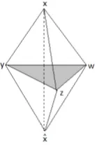
Example 2.2.1. We illustrate how construction of the complex with Stanley–Reisner ring

M =k[x,x, y, z, wˆ ]/hxx, yzwˆ i.

mirrors the generating of the corresponding Hilbert Function table by adding one variable

at a time and including all relevant monomials in the ideal used in the quotient.

Figure 2.1: 4-vertices, 3-edge, 0-faces

Start with the complex C0 corresponding to the point x we have the polynomial ring

k[x]. Bringing the next variable ˆx we have a new complex C1 corresponding to the

points x,xˆ. So we have k[x,xˆ]/hxxˆi. When the next variable y shows up we have the complex C2 corresponding to the points x,x, yˆ and the edges xy and ˆxy. By the same

way, whenz shows up we have the complex C3 corresponding to the points x,x, y, zˆ , the

edgesxy, xz, yz, yx, zˆ xˆand the facesxyz and yxzˆ . To generate the table below we invoke Theorem 2.1.1

HF{k[x]} 1 1 1 1 1 1 1 1 ...

LetM1 =k[x,x, y, zˆ ]/hxxˆi.

Then by using the short exact sequence (s.e.s.) for M we have

0 −→ b3j

inclusion

−−−−−→ b2j

multiply by w

−−−−−−−−−→ b1j −→ b0j −→ 0

0 −→ (0 :w)M(−1)

inclusion

−−−−−→ M(−1) −−−−−−−−−→multiply by w M −→ M/wM ∼=M1 −→ 0

0 0 0 1 1 0

0 0 1 5 4 0

0 0 5 14 9 0

0 1 14 29 16 0

0 4 29 50 25 0

0 9 50 77 36 0

0 16 77 110 49 0

0 25 110 149 64 0

... ... ... ... ... ...

... ... ... ... ... ...

The justification for the values in the left most column is based on the annihilator

(0 : w) ={q ∈M :qw = 0∈M}

associated with the map which is multiplication byw. A basis for the b-graded component of the module (0 :w) is the following set:

B = {nonzero p∈M2 of degreeb :yz|p}

= {(yz)(r) : nonzero r∈M1 with degreeb−2 and (xxˆ)-yzr}

= {(yz)(r) : nonzero r∈M1with degree b−2}.

Thus HF{(0 : w)} =|B| = HF{M1(−2)}. Having accounted for all annihilator elements

Example 2.2.2. We are looking for the Hilbert function on the module

M =k[x, y, z]/hx2yz3, x3z, y2z2i.

By rearranging the variables in our example we have thatM =k[y, z, x]/hy2_z2_{, x}2_yz3_{, x}3_zi

and based on Theorem 2.1.1 we have:

HF{k[y]} 1 1 1 1 1 1 1 1 ...

HF{k[y, z]/hy2_z2_{i}= HF{M}

1} 1 2 3 4 4 4 4 4 ...

Therefore, based on the short exact sequence we have

0 −→ (0 :x)(−1) −→M(−1)−→ M −→ M1 −→0

0 0 0 1 1 ={1} 0

0 0 1 3 2 ={y, z} 0

0 0 3 6 3 ={y2_{, yz, z}2_{} 0}

0 0 6 10 4 ={y3_{, y}2_{z, yz}2_{, z}3_{} 0}

0 1 ={x2z} 10 12 4 ={y4, y3z, yz3, z4} 0 0 2 ={yx2_{z, z}2_x2_{} 12 13 4 ={y}5_{, yz}4_{, y}4_{z, z}5_{} 0}

0 4 ={1, y2_x2_{z, yzx}2_{z, z}2_x2_{z} 13 14 4 0}

... ... ... ... ... ...

... ... ... ... ... ...

In order to figure out the Hilbert function of the annihilator module we need to find all

the non zero elements in M. Those elements should be either multiple of xyz3 or x2z. Therefore, we cannot have a factor of y and a factor of y2z. In other words, there are no elements in M1 that create x2yz3 and x3z. However, there are elements in M1 that

createy2_z2_{. By this way and using the fact that the alternating sum is zero we create the}

above table. In this example we can observe that the draw back is that computing the

Hilbert function of the annihilator ideal would require counting.With the next examples

2.3

Examples

In this section we use the basic results earlier in this chapter to find the Hilbert function

of key examples that provide the motivation for the techniques we develop in chapters 3

and 4. To be systematic we find it convenient to group the examples based on the number

of monomials generating the ideal used to produce the quotient ring.

2.3.1

The ideal used to produce the quotient polynomial ring is

a principal ideal

Consider M =k[x1, x2, . . . , xa]/hui where degu=d. Using Equation (2.1) we obtain the

following:

HF(M, b) =

      

F(a, b), for 0≤b ≤d−1

F(a, b)−F(a, b−d), for b≥d

(2.3)

This approach combined with the result in Proposition 2.1.2 immediately yields

HF(M, b) =

            

F(a, b) =

b

X

j=0

1

j![a−1]

j_{, for 0≤b≤d−1}

F(a, b)−F(a, b−d) =

b

X

j=b−(d−1)

1

j![a−1]

j

, for b ≥d

and this in turn can be encoded as matrix multiplication using an infinite matrix and

                          1

0! 0 0 0 0 0 0 0 ...

1 0!

1

1! 0 0 0 0 0 0 ...

1 0!

1 1!

1

2! 0 0 0 0 0 ...

.. . ... ... ... ... ... ... ... ... 1 0! 1 1! 1 2! 1 3! ... 1

(d−1)! 0 0 ...

0 1 1! 1 2! 1 3! ... 1 (d−1)!

1

d! 0 ...

0 0 _2!1 _3!1 ... _(d−1_{1)! d}1_{! (d+1)!}1 ... ... ... ... ... ... ... ... ... ... ... ... ... ... ... ... ... ... ...                           ·                          

[a−1]0 [a−1]1 [a−1]2 [a−1]3 [a−1]4 [a−1]5 [a−1]6

... ...                           =                          

HF(M,0) HF(M,1) HF(M,2)

.. .

HF(M,d−1) HF(M,d) HF(M,d+1)

.... ....                           .

In what follows we concentrate our efforts in finding ways to compute the Hilbert function

of a polynomial ring as finite sums and differences of the Pascal table row corresponding

to the number of variables in in our polynomial ring. In each such case one can do

as above and use Proposition 2.1.2 to produce a matrix multiplication approach similar

to the above. We’ll leave this for the reader to try using the methods in chapter four

as a starting point. Here are two examples to illustrate the above computations more

concretely.

Example 2.3.1. We are looking for the Hilbert function of the module

M =k[x, y, z]/hxy2_i.

Equation (2.3) indicates the following recurrence relation for this quotient ring

HF(M, b) =

      

F(a, b), for 0≤b≤2

Therefore, the Hilbert function of the module M = k[x, y, z]/hxy2i is expressed by the following sequence of numbers

HF(M, b): 1 3 6 9 12 15 18 ...

Finally, we can rewrite the second part of the above function as

F(a, b)−F(a, b−3) =

b

X

j=b−2

1

j![a]

j_{, forb ≥3.}

An alternative way to express the Hilbert function of R is given by the following way

                         

1 0 0 0 0 0 0 ...

1 _1!1 0 0 0 0 0 ...

1 1

1! 1

2! 0 0 0 0 ...

0 _1!1 _2!1 _3!1 0 0 0 ...

0 0 _2!1 _3!1 _4!1 0 0 ...

0 0 0 _3!1 _4!1 _5!1 0 ...

0 0 0 0 _4!1 _5!1 _6!1 ... ... ... ... ... ... ... ... ... ... ... ... ... ... ... ... ...                           ·                           2(0) 2(1) 2(2) 2(3) 2(4) 2(5) 2(6) ... ...                           =                           1 3 6 9 12 15 18 ... ...                           .

2.3.2

The ideal used in the quotient polynomial ring consists of

two monomials

observeu |q and v |q ⇔lcm(u, v) |q. Therefore with the use of the inclusion-exclusion principle we have

HF(hu, vi, b) = HF(hui, b) + HF(hvi, b)−HF(lcm(u, v), b).

Since every ideal on the right-hand side is a principal ideal we apply lemma 1.0.3 and

the “rank–nullity” reasoning from Chapter 1 to get after setting dlcm = deg(lcm(u, v)),

dmin = min(du, dv) and dmax= max(du, dv),

HF(M, b) =

                      

F(a, b), for 0≤b < dmin

F(a, b)−F(a, b−dmin) for dmin ≤b < dmax

F(a, b)−F(a, b−du)−F(a, b−dv) for dmax ≤b < dlcm

F(a, b)−F(a, b−du)−F(a, b−dv) +F(a, b−dlcm) for b ≥dlcm

Example 2.3.2. We are looking for the Hilbert function of the module

M =k[x, y, z]/hx2_{y, xz}2_i.

Equation (2.3) indicates the following recurrence relation for this quotient ring

HF(M, b) =

      

F(a, b), for 0≤b ≤2

F(a, b)−2F(a, b−3) +F(a, b−5), forb ≥3

Therefore, the Hilbert function of the module M = k[x, y, z]/hx2y, xz2i is expressed by the following sequence of numbers

HF(M, b): 1 3 6 8 9 10 11 ...

In the next chapter we make full use of the Principle of Inclusion and Exclusion to

of this example to illustrate an alternative which accounts for the monomials of degreeb

in the ideal only once. In other words, the principle of inclusion-exclusion is a sequence

of corrections for alternating over-counts and under-counts which corresponds to regions

of the Venn diagram where two, three, four, etc... sets overlaps. Our goal here is to

partition the union of all sets in the Venn diagram into disjoint sets as to avoid alternating

inclusions with exclusions. This is accomplished by ordering our setsE1, E2, E3, . . . then

lettingF1 =E1, F2 =E2\F1, F3 =E3 \(F1∪F2), . . .. This is an approach conceptually

similar to the Gramm-Schmidt process in linear algebra.

Letu=x2y and v =xz2. Let also E1 =hui and E2 =hvithen F1 =E1

and F2 = {all monomials which are multiple of v but not ofu}. Since E1 and E2 are

graded modules thenF1 andF2 will be graded sets. For example, for degree 4,E1 and E2

are disjoint so no monomials of degree 4 needs to be excludes forF2. However, for degree

5, for example uz2 _{= vxy; in this case we want to count x}2_yz2 _{as a multiple of u (i.e.}

belonging to F1) but prevent it being counted as a multiple ofv. So we want to disallow

in this case the factorxy from being multiplied by v. Observe

lcm(x2_y,xz2₎

xz2 =

x2_yz2

xz2 =xy

which is known as a syzygy. How this would work with example 2.3.2 illustrated up to

degree 6 in the following table,where

Degree k 0 1 2 3 4 5 6 ...

HF{k[x,y,z]} 1 3 6 10 15 21 28 ...

F1 u ux, uy, uz, ux2, uy2, uz2, ux3, uy3, uz3, xyzu, ...

uxy, uyz, uxz ux2y, uxy2, ux2z, ...

uy2z, uxz2, uyz2 ...

F2 v vx, vy, vz vx2, vy2, vz2, vx3, vy3, vz3, ...

xzv, yzv vx2_{z, vy}2_{z, vxz}2_{, vyz}2 _...

|F1| 1 3 6 10 ...

|F2| 1 3 5 7 ...

Chapter 3

LCM–Lattice Method

As discussed at the end of the previous the challenge remains to find the Hilbert function

of a monomial ideal with more than one monomial generator. Our first approach, which

we develop in this chapter, uses the well known Principle of Inclusion and Exclusion

(which the reader will find in the standard reference [4]). First we need the following:

Proposition 3.0.1. hui ∩ hvi=hlcm(u, v)i

Proof. p∈ hui ∩ hvi ⇔u|p and v |p⇔lcm(u, v)|p

Corollary 3.0.1. hp1i ∩ hp2i ∩ hp3i ∩...∩ hpri=hlcm(p1, p2, p3, ..., pr)i

Proof. (By Induction)

• The above proposition is the above case.

• Suppose

r−1

\

i=1

hpii=hlcm(p1, p2, p3, ..., pr−1)i then

r

\

i=1

hpii= r−1

\

i=1

Further use of enclusion-exclusion; this time with n monomials we get

HF(hp1, p2, p3, ..., pni, b) = |{monomials of degree b in hp1, p2, p3, ..., pni}|

= |{monomials of degree b in hp1iOR hp2i OR... ORhpni}|

= X

1≤j1≤n

|hpj1i| −

X

1≤j1<j2≤n

|hlcm(pj1, pj2)i|

+ X

1≤j1<j2<j3≤n

h(pj1, pj2, pj3)i|

+...

+(−1)r−1 X

1≤j1<j2<...<jr≤n

|hlcm(pj1, pj2, ..., pjr)i| +(−1)n−1|hlcm(p1, p2, ..., pn)i|

=

n

X

r=1

(−1)r−1 X

1≤j1<j2<...<jr≤n

|hlcm(pj1, pj2, ..., pjr)i|

!

.

Assigningdj1j2j3...jr = deg(lcm(p1, p2, p3, ..., pr)), where 1≤r≤n and

1≤j1 < j2 < j3 < ... < jr ≤n. To facilitate expressing the Hilbert function let’s expand F(a, b) = 0 if b <0.

Then HF(hp1, p2, p3, ..., pni, b) = n

X

r=1

(−1)n−1 X

1≤j1<j2<...<jr≤n

F(a, b−dj1j2j3...jr)

!

and

HF(k[¯x]/hp1, p2, p3, ..., pri, b) = F(a, b)− n

X

r=1

(−1)n−1 X

1≤j1<j2<...<jr≤n

F(a, b−dj1j2j3...jr)

!

.

The argument starting at the top of this page proves the validity of the method we now

describe. The starting point of building up the lcm–lattice is what we call layer 1. Layer

1 is a row containing all the monomials of the given ideal. Finding the lcm of all the pairs

the given ideal. The last layer will contain the lcm of all the monomials given in the ideal.

If the ideal I contains n monomials then the number of monomials in the lcm-lattice in layers 1, 2, 3, ..., n will be

n

1

,

n

2

,

n

3

, . . . ,

n n

correspondingly. These values are

those found in thenth _{row of the Pascal triangle to the right and including}

n

1

.

The following examples give a nice view of the above description.

Example 3.0.3. Finding the Hilbert function of the module M =R/hx2, y3i where R =

k[x, y, z].

In the case that we have two monomials in the ideal the lcm lattice is simple. Start by

building up the lcm lattice. Layer 1 is called the row that has all the monomials of the

ideal. Afterwards, we take the lcm of the two monomials and we have the following

x2 y3 layer 1

x2y3 layer 2

According now to the above lcm lattice, we are left with a lattice of monomials on which

we use inclusion - exclusion at each row to produce the alternating sum that computed

HF{R} layer 1(-) layer 2(+) HF{M}

1 0 0 0 1

3 0 0 0 3

6 -1 0 0 5

10 -3 -1 0 6

15 -6 -3 0 6

21 -10 -6 1 6

28 -15 -10 3 6

36 -21 -15 6 6

45 -28 -21 10 6

55 -36 -28 15 6

.. .. .. .. ..

.. .. .. .. ..

We apply now our lcm–Lattice method to quotient rings where the monomial ideal consists

of three monomials.

Example 3.0.4. Given the quotient ring M = k[x, y, z]/hxz, yz, x2yi, find its Hilbert function.

Start by building up the lcm lattice.

x2_{y xz yz layer 1}

x2_{yz x}2_{yz xyz layer 2}

x2_{yz layer 3}

So we are left with the above lattice of monomials on which we use inclusion - exclusion

at each row to produce the alternating sum that computed the Hilbert function. Let

the alternating sum is zero. Therefore, the monomials that are cancelled are displayed in

bold-faced. By this way we have the following

HF{R} layer 1(-) layer 2(+) HF{M}

1 0 0 1

3 0 0 3

6 -2 0 4

10 -6 0 4

15 -12 1 4

21 -20 3 4

28 -30 6 4

36 -42 10 4

45 -56 15 4

55 -72 21 4

.. .. .. ..

.. .. .. ..

Example 3.0.5. Compute the Hilbert function of the module

M =k[x, y, z]/hx2_y3_{z, xz}3_{, xy}4_{z, x}2_z2_{i. As before, for the sake of simplicity, we will let}

R=k[x, y, z].

Start by building up the lcm lattice and we have

x2y3z xz3 xy4z x2z2 layer 1

x2y3z3 x2y4z x2y3z2 xy4z3 x2z3 x2y4z2 layer 2 x2_y4_z3 _x2_y3_z3 _x2_y4_z3 _x2_y4_z2 _{layer 3}

We typeset in bold face the monomials that are cancelled. By that way we have the

following the table

HF{R} layer 1 layer 2 layer 3 HF{M}

1 0 0 0 0 0 0 1

3 0 0 0 0 0 0 3

6 0 0 0 0 0 0 6

10 0 0 0 0 0 0 10

15 -2 0 0 0 0 0 13

21 -6 0 1 0 0 0 16

28 -12 -2 3 0 0 0 17

36 -20 -6 6 2 0 0 18

45 -30 -12 10 6 1 0 20

55 -42 -20 15 12 3 -1 22

.. .. .. .. .. .. .. ..

.. .. .. .. .. .. .. ..

In Chapter 4 we develop an alternative approach based on the Syzygy of pairs of

Chapter 4

The Syzygy Method

In this chapter we extend the second approach to the example 2.3.2 to handle ideals with

finitely many monomials as generators. When implemented as a recursive algorithm this

method will break down a Hilbert function computation into a sum–difference expression

of Hilbert functions all of which involve a principal ideals. The computation is finished by

invoking Corollary 2.3. Unlike the lcm–method, the principal ideals used will be generated

by always taking syzygys of pairs of monomials (we never consider three or more of the

given monomials in a computational step). The key recursive step is given by the following

theorem.

Theorem 4.0.1. (Syzygy method) LetM =k[¯x]/I, whereI =hp1, p2, p3, ..., pri, a

mono-mial ideal generated by p1, p2, p3, ..., pr∈k[¯x]. Then, using the notation dj = deg(pj) and mij = lcm(pi,pj)

pj ∈k[¯x] with i < j, we have

HF(M, t) =F(a, t)−F(a, t−d1)−

r

X

j=2

HF(k[¯x]/hm1j, m2j, m3j, ..., m(j−1)ji, t−dj).

Proof. (By Induction)

• Suppose r >1 and

HF(k[¯x]/hp1, p2, p3, ..., pr−1i, t) = F(a, t)−F(a, t−d1)

−

r−1

X

j=2

HF(k[¯x]/hm1j, m2j, m3j, ..., m(j−1)ji, t−dj).

• We show that

HF(k[¯x]/hp1, p2, p3, ..., pri, t) = HF(k[¯x]/hp1, p2, p3, ..., pr−1i, t)

−HF(k[¯x]/hm1r, m2r, m3r, ..., m(r−1)ri, t−dr).

A monomialq∈k[¯x], of degreetrepresent a nonzero element ink[¯x]/hp1, p2, p3, ..., pr−1i

and is zero in k[¯x]/hp1, p2, p3, ..., pri if and only ifpi -q for all

1≤i < r and pr|q. If we call the set of all such monomials Γ(t) then we have that HF(k[¯x]/hp1, p2, p3, ..., pri, t) = HF(k[¯x]/hp1, p2, p3, ..., pr−1i, t)− |Γ(t)|.

A monomial q ∈ k[¯x] satisfies q ∈ Γ(t) ⇔ q = a·pr where a is a monomial in k[¯x]

of degree t−dr and pi - a·pr for all 1 ≤i < r. This is equivalent to mir -a for all

1≤i < r.

Since a is a monomial we have that,

a /∈ hmiri, for all 1≤i≤r−1

⇔a /∈ hm1r, m2r, m3r, ..., m(r−1)ri

⇔a∈k[¯x]/hm1r, m2r, m3r, ..., m(r−1)ri.

we only need to observe that a is uniquely determined by q∈Γ(t) and every

a ∈k[¯x]/hm1r, m2r, m3r, ..., m(r−1)ri uniquely determines a monomial q.

Example 4.0.6. Both the lcm-lattice-method and the Syzygy method produce similar

for-mulas for computing the Hilbert function. We apply the Syzygy method to establish that the

lcm-lattice method holds for a monomial ideal with three monomials. The reader should

observe that this will confirm of that result without the use of inclusion-exclusion.

ConsiderI generated by three (not necessarily distinct) monomialsp1, p2, p3 with degrees

d1, d2, d3 respectively. We need to show that

HF{k[¯x]/hp1, p2, p3i} = F(a, t)−F(a, t−deg(p1))

−F(a, t−deg(p2))−F(a, t−deg(p3))

+F(a, t−deg(lcm(p1, p2))) +F(a, t−deg(lcm(p2, p3)))

+F(a, t−deg(lcm(p1, p3)))−F(a, t−deg(lcm(p1, p2, p3))).

By the syzygy method we obtain the following equality which we call the syzygy equality

HF{k[¯x]/hp1, p2, p3i} = F(a, t)−F(a, t−d1)−HF{k[¯x]/hm12i(−d2)}

−HF{k[¯x]/hm13, m23i(−d3)}

Applying the syzygy method to the third and fourth summands on the right hand side

we have

HF{k[¯x]/hm12i(−d2)} = F(a, t−d2)−F(a, t−d2−deg(m12))

and

HF{k[¯x]/hm12, m23i(−d3)} = F(a, t−d3)−F(a, t−d3−deg(m13))

−HF k[¯x]/lcm(m13, m23)m−231

(−d3−deg(m23)) .

and

HF{k[¯x]/hlcm(m13,m23)

m23 i(−d3−deg(m23))}=

= F(a, t−d3−deg(m23)−F

a, t−d3−deg(m23)−deg

lcm(m13, m23

m23

= F(a, t−deg(lcm(p2, p3)))−F(a, t−d3−deglcm(m13, m23))

= F(a, t−deg(lcm(p2, p3)))−F(a, t−(d3+ deglcm(m13, m23))

= F(a, t−deg(lcm(p2, p3)))−F

a, t−(deg(p3) + deg

lcm

lcm(p1, p3)

p3

,lcm(p2, p3) p3

= F(a, t−deg(lcm(p2, p3)))−F

a, t−

deg(p3) + deg

lcm(p1, p2, p3)

p3

= F(a, t−deg(lcm(p2, p3)))−F(a, t−deg(lcm(p1, p2, p3)))).

Back substituting the iterated results of Syzygy method into the Syzygy equation we get

the same alternating sum produced by lcm-method.

Thus providing the lcm-lattice method valid.

The following examples are based on the Syzygy method.

Example 4.0.7. Find the Hilbert function of M =R/hx2_{, y}3_{i, where R=k[x, y, z].}

We will only need the syzygy m12 = lcm(x

2_,y3₎

y3 =

x2_y3

y3 = x2. Computing the Hilbert function in this case requires only one use Theorem 4.0.1, which yields the following:

Based on the Corollary 1.0.3 we see that the last term in 4.1 it is shifted by 3, so we have

HF{R/hx2i(−3)} = HF{R(−3)} −HF{R(−deg(x2))(−3)}

= HF{R(−3)} −HF{R(−5)}. (4.2)

Therefore, by substituting 4.2 into 4.1, we have

HF{M} = HF{R} −HF{R(−2)} −[HF{R(−3)} −HF{R(−5)}] = HF{R} −HF{R(−2)} −HF{R(−3)}+ HF{R(−5)}.

The Hilbert function ofM shows in the last column of the following row-generating table HF{R} −HF{R(−2)} -HF{R(-3)} HF{R(-5)} HF{M}

1 0 0 0 1

3 0 0 0 3

6 -1 0 0 5

10 -3 -1 0 6

15 -6 -3 0 6

21 -10 -6 1 6

28 -15 -10 3 6

36 -21 -15 6 6

45 -28 -21 10 6

55 -36 -28 15 6

66 -45 -36 21 6

78 -55 -45 28 6

.. .. .. .. ..

Now apply the Syzygy method to quotient rings whose monomial ideal consists of three

monomials.

Example 4.0.8. Finding the Hilbert function of the quotient ringM =k[x, y, z]/hxz, yz, x2yi.

m12 = lcm(_yzxz,yz) = xyz_yz =x,

m13 = lcm(xz,x

2_y)

x2_y =

x2_yz

x2_y =z,

m23 = lcm(yz,x

2_y)

x2_y =

x2_yz

x2_y =z. LetR =k[x, y, z].

Using now the syzygy method we can express the Hilbert function ofM as follows

HF{M} = HF{R} −HF{R(−deg(xz))} −HF{R/hm12i(−deg(yz))}

−HF{R/hm13, m23i(−deg(x2y))}

= HF{R} −HF{R(−2)} −HF{R/hxi(−2)} −HF{R/hzi(−3)}. (4.3)

Observe that the last two terms of 4.3 are equal to the second row of the Pascal table just

shifted since

HF{R/hxi(−2)} ∼= HF{k[y, z](−2)}

and

HF{R/hzi(−3)} ∼= HF{k[x, y](−3)}.

HF{R} −HF{R(−2)} −HF{R/hxi(−2)} −HF{R/hzi(−3)} HF{M}

1 0 0 0 1

3 0 0 0 3

6 -1 -1 0 4

10 -3 -2 -1 4

15 -6 -3 -2 4

21 -10 -4 -3 4

28 -15 -5 -4 4

36 -21 -6 -5 4

45 -28 -7 -6 4

55 -36 -8 -7 4

66 -45 -9 -8 4

78 -55 -10 -9 4

.. .. .. .. ..

.. .. .. .. ..

Example 4.0.9. Compute the Hilbert function of the module

M =k[x, y, z]/hx2z2, xz3, xy4z, x2y3zi. As before let R=k[x, y, z]. By finding now the syzygies, we have

m12= x

2_z3

xz3 =x,

m13= x

2_y4_z2

xy4_z =xz,

m23 = xy

4_z3

xy4_z =z2,

m14= x

2_y3_z2

x2_y3_z =z,

m24 = x

2_y3_z3

x2_y3_z =z

2_,

m34= x

2_y4_z

Based on the syzygy method we have

HF{M} = HF{R} −HF{R(−deg(x2z2))} −HF{R/hxi(−deg(xz3))}

−HF{R/hxz, z2i(−deg(xy4z))} −HF{R/hz, z2, yi(−deg(x2y3z))}

= HF{R} −HF{R(−4)} −HF{R/hxi(−4))} −HF{R/hxz, z2i(−6)}

−HF{R/hz, z2, yi(−6)}. (4.4)

From 4.4 we can see that

HF{R/hxi(−4)} ∼= HF{k[y, z](−4)} (4.5)

and

HF{R/hz, z2, yi(−6)} ∼= HF{R/hy, zi(−6)} ∼= HF{k[x](−6)}. (4.6)

Therefore, 4.5 is given by the 2nd row of the Pacal table shifted down by four and 4.6 is

given by the 1st row shifted down by six.

Moreover, in order to find Hilbert function ofM we need to find the HF{R/hxz, z2_i(−6)}.

Applying again the syzygy method to the fourth summand on the right hand side of 4.4

we have that

m12= xz

2

z2 =x.

Observe that the shifting is equally distributed in all the terms as follows

HF{R/hxz, z2i(−6)} = HF{R(−6)} −HF{R(−deg(xz))(−6)} −HF{R/hxi(−deg(z2))(−6)}

= HF{R(−6)} −HF{R(−2)(−6)} −HF{R/hxi(−2)(−6)}

This way we have the following row-generating table

HF{R(−6)} −HF{R(−8)} −HF{k[y, z](−8)} HF{R/hxz, z2_i(−6)}

0 0 0 0

0 0 0 0

0 0 0 0

0 0 0 0

0 0 0 0

0 0 0 0

1 0 0 1

3 0 0 3

6 -1 -1 4

10 -3 -2 5

15 -6 -3 6

.. .. .. ..

.. .. .. ..

Substituting now 4.5,4.6,4.7 into 4.4 we have

HF{R} −HF{R(−4)} −HF{k[y, z](−4)} −HF{R/hxz, z2_{i(−6)} −HF{k[x](−6)} HF{M}}

1 0 0 0 0 1

3 0 0 0 0 3

6 0 0 0 0 6

10 0 0 0 0 10

15 1 1 0 0 13

21 -3 -2 0 0 16

28 -6 -3 -1 -1 17

36 -10 -4 -3 -1 18

45 -15 -5 -4 -1 20

55 -21 -6 -5 -1 22

66 -28 -7 -6 -1 24

.. .. .. .. .. ..

.. .. .. .. .. ..

Chapter 5

Syzygy method via homological

algebra

The short exact sequence that involvesφxa := multiplication byxa (see [5] page 98) works well with the assemblage row-by-row of a Hilbert function table. That is because the key

homomorphism in the short exact sequence is multiplication by a variable followed by

natural projection. Consequently the last non-zero object of the short exact sequence is

the cokernel of φxa. This cokernel (we saw in chapter 2) turns out to be the quotient ring corresponding to the row in the Hilbert function table immediately preceding the

introduction of the variablexa. In other words, of the two Hilbert function sequences that

the short exact sequence needs to generate the the Hilbert function of k[x1, x2, ..., xa]/Ia,

one of them (the right-most) is the Hilbert function of k[x1, x2, ..., xa−1]/Ia−1. Therefore

any remaining difficulty would be confined to finding the Hilbert function for the kernel

of φxa.

variables to an infinite set of variables x1, x2, ..., xd, xd+1, .... For integer value a let

Sa ={pi ∈S :pi ∈k[x1, x2, ..., xa]}. Re-index if necessary the set S such that

1. S_a0 ⊂Sa if a0 ≥a and ...

2. For pi, pj ∈Sa, j > i only if the highest power ofxa dividingpi also divides pj.

The reader should observe that the first requirement of this re-indexing of the generators

ofI has the purpose of introducing the generators for the idealsIain consecutive order as the variables xa are introduced one-by-one. The second criteria for the re-index ensures

that, as the set Sa−1 is enlarged to Sa, the new monomials are ordered in (non-strict)

increasing order of the power of xa. This second criteria is done to ensure that the

variable xa does not appear in the syzygies we might need compute as we generate the ath_{-row of the Hilbert table. Also observe that if S}

a = ∅ then set Ia = 0; otherwise set Ia = hpi|pi ∈ Sai. Let Ma = k[x1, x2, ..., xa]/Ia. Construct an infinite array whose ath

row is the sequence of Hilbert function values ofMa.

Consider the followingshort exact sequence whereφxa is multiplication byxa, the module

Ma=k[x1, x2, . . . , xa]/Ia, and (0 :xa)Ma = kerφxa ,

0→(0 :xa)Ma(−1)→Ma(−1)

φxa

→ Ma→Ma/xaMa →0.

Set S0 =∅ and for a≥1, if Sa−1 (Sa set

Uxa ={qi =

pi xa

: pi ∈Sa\Sa−1}.

IfSa−1 =Sa then set Uxa =∅.

Lemma 5.0.1. (0 :xa)Ma =hqi :qi ∈UxaiMa.

IfUxa 6=∅ the following equivalence holds:

xag = 0 inMa ⇔pi |xag for some pi ∈Sa\Sa−1

⇔qi |g for some qi ∈Uxa

⇔g ∈ hqi : qi ∈Uxai

Remark 5.0.1. Observe that if Uxa =∅ then from the above lemma follows that (0 :xa)Ma = 0.

Using the same notation for syzygies as in the previous chapter, namely mij =

lcm(pi,pj)

pj we now state the following lemma.

Lemma 5.0.2. A non-zero monomial g ∈ (0 : xa)Ma can be written as follows for one and only one qi ∈Uxa,

1. g =α1q1 if q1 ∈Uxa

2. g =αjqj if qj ∈Uxa and mij -αj for all 1≥i < j

and conversely any g satisfying one of the equations above, belongs to (0 :xa)Ma.

Proof. By the previous lemma all we are left to show is uniqueness.

Supposeg ∈(0 :xa)Ma, letibe the smallest index such thatqi |g. Then for any 1≥i

0 _{< i,}

g cannot be written as g =αi0q_i0.

Ifi < j and qj |g then

αj = g qj

but qi |g and qj |g ⇒lcm(qi, qj)|g

⇔ lcm(qi, qj)

qj | g

Theorem 5.0.2. With the notation of the two lemmas above, the Hilbert function of the

annihilator of the homomorphism φxa satisfies the following formula,

HF{(0 : xa)Ma}=δ(a)HF{k[x1, x2, . . . , xa−1](−degq1)}

+ X

1<j∈Index SetUxa

HF{k[x1, x2, . . . , xa−1]/hm1j, m2j, . . . , m(j−1)ji(−degqj)}

where δ(a) = 0 for q1 ∈/ Uxa, and δ(a) = 1 for q1 ∈Uxa.

Proof. Ifq1 ∈Uxa and q1 |g then α1 ∈k[x1, x1, . . . , xa−1]/Ia−1 and deg(a1) =b−deg(q1). But sinceUxa−1 =∅, thenIa−1 = 0 which gives us the summand withδ(a) = 1.

Ifq1 ∈/ Uxa then δ(a) = 0 and the first summand is irrelevant.

Moreover, for all g ∈(0 :xa)Ma expressible as g =αjqj with mij -αj, 1≥i < j, then

αj ∈(k[x1, x2, . . . , xa−1]/Ia−1)/hm1j, m2j, . . . , m(j−1)ji

∼

=k[x1, x2, . . . , xa−1]/hm1j, m2j, . . . , m(j−1)ji.

The last isomorphism being due to the second and third isomorphism theorems.

Remark 5.0.2. Observe that if Uxa =∅ then the sum in the theorem is zero, i.e. HF ((0 :xa)Ma, b) = 0 for all b≥0.

With the Hilbert function for the annihilator (0 : xa)Ma and the Hilbert function for

Ma/xaMa ∼= Ma1 in hand it is straightforward to implement the procedure outlined in chapter 2 to generate the Hilbert function of Ma. For that reason we only show in the

next example how to write the Hilbert function of the annihilator in terms of the Hilbert

function of simpler quotient rings.

Example 5.0.10. Use the above theorem to write a sum equivalent to the non-trivial

annihilator ideals (0 : xa)Ma, where I = hy

6_{, x}3_y5_{, x}2_y2_z2_{, x}3_{z, x}2_yz3_{i where the variables}

Before embarking in the computations we consider if the set of generators of I needs re-indexing given the order we have chosen to introduce the variables (this order is quirky

in that the variable y is introduced before the variable x – and was chosen to illustrate we are free to select the order in which the variables are introduced). The criteria that

S_a0 ⊂ Sa if a0 ≥ a is satisfied by the order in which the monomials generating I are

listed. However the second criteria; namely, that for pi, pj ∈Sa, j > ionly if the highest

power of xa dividing pi also divides pj, requires that the order of the monomials x2y2z2

and X3z be swapped. Observe that adjusting the indexing to satisfy the second criteria does not interfere with the first criteria. In other words, after swapping the third and

fourth monomials we getI =hy6, x3y5, x3z, x2y2z2, x2yz3iwhich satisfies both re-indexing criteria. The first annihilator is (0 :y)My, whereMy =k[y]/hy

6_i.

In this caseUy ={y5} and

HF{(0 : y)My}= HF{k(−5)}.

The second annihilator is (0 :x)Mx where Mx=k[y, x]/hy

6_{, x}3_y5_{i. In this case}

Ux ={x2y5} and there is only the syzygy m12 =y to consider. Therefore,

HF{(0 : x)Mx}= HF{k[y]/hyi(−7)}= HF{k(−7)}.

The third and last non-trivial annihilator is (0 :z)Mz, where

In this caseUz ={x3, x2y2z, x2yz2}. The syzygies to consider are

m13=y6 m23=y5

m14=y4 m24=xy3 m34 =x

m15=y5 m25=xy4 m35 =x m45=y.

Therefore,

HF{(0 : z)Mz}=HF{k[y, x]/hy

6_{, y}5_i(−3)}

+ HF{k[y, x]/hy4, xy3, xi(−5)}

+ HF{k[y, x]/hy5, xy4, x, yi(−5)}

=HF{k[y, x]/hy5i(−3)}

+ HF{k[y]/hy4i(−5)}+ HF{k(−5)}.

As the reader can see this approach is quite close in spirit to the Syzygy method discussed

in the previous chapter. The only significant difference is in the tools used to prove

it. All the information about the Hilbert function was obtain from the syzygies. We

must conclude that we have developed two different approaches to computing the Hilbert

Bibliography

[1] Margherita Barile and Eric W. Weisstein. Hilbert Function.

http://mathworld.wolfram.com/HilbertFunction.html.

[2] Richard M. Foote David S. Dummit. Abstract Algebra, 3rd Edition. John Wiley and

Sons, INC., 2003.

[3] D Eisenbud. Commutative Algebra with a View toward Algebraic Geometry.

Springer-Verlag, 1995.

[4] R. M. Wilson J. H. van Lint. A Course in Combinatorics. Cambridge University

Press, 1992.