On model, algorithms and experiment for micro-doppler based recognition of ballistic targets

On Model, Algorithms, and

Experiment for

Micro-Doppler-Based

Recognition of Ballistic Targets

ADRIANO ROSARIO PERSICO, Student Member, IEEE CARMINE CLEMENTE, Member, IEEE

DOMENICO GAGLIONE, Student Member, IEEE CHRISTOS V. ILIOUDIS, Student Member, IEEE JIANLIN CAO, Student Member, IEEE

University of Strathclyde, Glasgow, U.K.

LUCA PALLOTTA, Member, IEEE

University of Naples Federico II, Naples, Italy

ANTONIO DE MAIO, Fellow, IEEE

Universit`a degli Studi di Napoli “Federico II”, Napoli, Italy

IAN PROUDLER

Loughborough University, Leicestershire, U.K.

JOHN J. SORAGHAN, Senior Member, IEEE

University of Strathclyde, Glasgow, U.K.

The ability to discriminate between ballistic missile warheads and confusing objects is an important topic from different points of view. In particular, the high cost of the interceptors with respect to tac-tical missiles may lead to an ammunition problem. Moreover, since the time interval in which the defense system can intercept the mis-sile is very short with respect to target velocities, it is fundamental to

Manuscript received September 3, 2015; revised February 1, 2016 and July 4, 2016; released for publication August 30, 2016. Date of publication February 7, 2017; date of current version June 7, 2017.

DOI. No. 10.1109/TAES.2017.2665258

Refereeing of this contribution was handled by R. Adve.

This work was supported by the Engineering and Physical Sciences Re-search Council under Grant EP/K014307/1.

Authors’ addresses: A. R. Persico, C. Clemente, D. Gaglione, C. V. Il-ioudis, J. Cao, and J. J. Soraghan are with the Centre for Excellence in Signal and Image Processing, University of Strathclyde, Glasgow, G1 1XW, U.K., (E-mail: [email protected]; carmine.clemente@ strath.ac.uk; [email protected]; [email protected]; [email protected]; [email protected]); L. Pallotta is with the CNIT, University of Naples Federico II, Naples, 80138, Italy, (E-mail: [email protected]); A. De Maio is with the Dipartimento di Ingegne-ria Elettrica e delle Tecnologie dell’Informazione, Universit`a degli Studi di Napoli “Federico II”, Via Claudio 21, I-80125 Napoli, Italy, (E-mail: [email protected]); I. Proudler is with the School of Electronic, Electrical and Systems Engineering, Loughborough University, Leicestershire LE11 3TU, U.K., (E-mail: [email protected]).

0018-9251/16C _{2017 CCBY}

minimize the number of shoots per kill. For this reason, a reliable tech-nique to classify warheads and confusing objects is required. In the efficient warhead classification system presented in this paper, a model and a robust framework is developed, which incorporates different micro-Doppler-based classification techniques. The reliability of the proposed framework is tested on both simulated and real data. I. INTRODUCTION

The challenge of ballistic missiles (BM) classification is continuing to grow in importance [1]. In particular, two principal factors increase the interest in developing efficient techniques to recognize missiles. The first is economic, because the interceptor missiles are expensive relative to that of tactical missiles. The second factor is tactical and relates to the possibility that there may be numerous missiles and many more objects present. Hence the defense system will have, in general, a limited number of missiles and consequently it is important to maximize the interception success ratio. Another fundamental aspect is that the period in which the missile can be intercepted by the defense system is limited, then it is necessary to recognize the real threats in a cloud of debris and other objects. The detection and recognition of a BM are challenging due to various reasons during different phases of its flight. Generally, a BM trajectory is divided into three parts [2]: boost phase, which comprises the powered flight portion; midcourse phase, which comprises the free-flight portion that constitutes most of the flight time and during which the missile separates from the rest of missile; and the re-entry phase wherein the warhead re-enters the Earth’s atmosphere to approach the target. As well as the warhead, the missile releases also confusing objects in order to make the BM detection more difficult for defense systems. These objects come in many different shapes.

can be used for the purpose of information extraction for target classification, because different behaviors produce different signatures [5].

In the last decade, a large amount of research has been conducted on the possibility to use micro-Doppler infor-mation to identify different targets in many fields of inter-est, e.g., human motion classification [6] and air moving target recognition [7]. Most systems use information ex-tracted from the time-frequency distribution (TFD) of radar echoes. In [6], [8], and [9], the features for human motion classification are empirically estimated from the spectro-gram. In [10], a set of features is evaluated by using the singular value decomposition (SVD) on the spectrograms and estimating the standard deviation of the first right sin-gular vector. In [11], Molchanov et al. propose a method for the extraction of cepstrum- and bicoherence-based features from TFD for aircraft classification. In [12], the features are estimated as the Fourier series coefficients of the spectro-gram envelope, whereas in [13] the mel-frequency cepstral coefficients (MFCC) are employed with the main aim to recognize human falling from other motions, which can be used for healthcare applications. Other features that are not extracted from TFD are presented in [7], where a method that employs empirical mode decomposition (EMD) and CLEAN technique is proposed. Moreover, a Greedy Gaus-sian mixture model based classification technique for ATR with low resolution ground surveillance radars is presented in [14], where the linear predictive coding (LPC) and cep-strum coefficient feature sets are extracted from the data. A micro-Doppler classification method that uses the strongest parts of the cadence velocity diagram (CVD) [15] for the feature vector construction is described in [16]. The algo-rithm is tested successfully in the case of the discrimination of human motions. However, it requires high storage ca-pabilities as long as the feature vector is composed by the highest cadence frequencies and sampled velocity profiles corresponding to each of them.

The aim of this paper is to demonstrate the capability and reliability of micro-Doppler information [17] for the discrimination between warheads and confusing objects. The determination of the best classification technique is outside the scope of this paper. Instead, we consider three typical techniques that exhibit different properties. In order to understand the micro-Doppler shifts, a high frequency based signal model for the targets of interest is proposed that incorporates the effects of occlusion for all the scat-tering points. A framework is presented for radar micro-Doppler classification based on the processing of the CVD with different information extraction techniques. In partic-ular, three different techniques for feature extraction from the CVD are presented. The first approach is based on the statistical characteristics of the unit area function obtained by averaging and normalizing the CVD (ACVD). The sec-ond method is based on the use of pseudo-Zernike (pZ) moments [5], [18]–[20], and the third one is based on the use of the Gabor filter [21]. The ACVD approach is known to require less computation compared to the other two methods, since a smaller feature vector dimension is used.

The pZ moments are widely used in image processing for pattern recognition due to their useful properties, such as scale, translation, and rotation invariance. In [5], a micro-Doppler-based framework using pZ moments has been pre-sented for classification of human movement. It has been compared with other common classification techniques un-derlining its better performance. Moreover, the scale invari-ant property is importinvari-ant for micro-Doppler-based feature due to their more robustness with respect to the angle of view, which affects strictly the maximum frequency shift. Gabor filters have been successfully employed to extract reliable features in several challenges, such as the texture and symbol classification [22], [23] and in the context of face recognition [24], especially due to their scale, transla-tion, rotatransla-tion, and illumination invariant properties. The last two types of features are selected for their high accuracy of performance. Moreover, since a work on successfully employment of Gabor filter for ballistic target classifica-tion has been presented in [21], the methods is taken as term of comparison extending the previous work with the application on simulated data and Booster data.

The remainder of the paper is organized as follows. Section II introduces the model for the signal received from BM warheads and confusing object. Section III describes the different feature extraction algorithms. In Section IV, both the simulated and the real dataset used to test the pro-posed algorithms are described. In Section VI, the effec-tiveness of the proposed approach is demonstrated showing the classification results on both simulated and real data. Section VI concludes the paper.

II. SIGNAL MODEL

In this section, the model for the signal scattered from a ballistic target is described. The exact calculation of the re-ceived radar signal from a target is usually very difficult be-cause of the scattering mechanisms, even if the geometrical shape of the object is simple. However, for high frequency radar systems, the received signal can be modeled approx-imately by a sum of signals received from some dominant and discrete scattering points on the target. These scattering points provide a concise and useful description of the object for the target recognition [3].

Without loss of generality and neglecting the envelope of the transmitted signal, it is assumed that the radar trans-mits a signal, which may be written as

stx(t)=exp(j2πf0t) (1)

wheref0is the radar carrier frequency. The generic received

signal can be written as

srx(t)= Ns−1

i=0

μi(t) exp(j2πf0(t−τi(t)) (2)

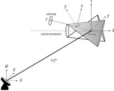
Fig. 1. Reference systems for ballistic targets.

the radar LOS (line of sight) and the symmetry axis of the target. Its value is 1 when there is a LOS for the scattering points, and 0 otherwise. An expression of the propagation delay for the generic point is given by

τi(t)= 2ρi(t)

c (3)

where c=3×108 m/s represents the speed of light in vacuum and ρi(t) is the distance between the radar and the considered point.

Considering three reference systems, as Fig. 1 illus-trates: the principal reference system ( ˆU ,V ,ˆ Wˆ), centerd on the radar; the natural coordinate system ( ˆX,Y ,ˆ Zˆ), which is parallel to the previous one and whose origin is thecenter of mass of the target; the local system ( ˆx,y,ˆ zˆ) such that the axis ˆz corresponds with the symmetry axis of target [2].

The distance ρi(t) is the norm of the position vector

rradar

i , i.e.,

ρi(t)= rradari =rradarcm +vt+ri(t) (4)

where rradar

cm is the initial position vector of the mass center with respect to the system ( ˆU ,V ,ˆ Wˆ),vis the translation velocity of the target and ri(t) is the position of the consid-ered point with respect to the ( ˆX,Y ,ˆ Zˆ) system.

Neglecting the time dependence for conciseness, rican be written as the following column vector

ri =(Xt, Yt, Zt)T = TmRt0

rlocal_p −rlocal_cm (5)

where (·)T _{is the transpose operator, Rt}

0is the Euler matrix that sets the position of the target with respect to the second system ( ˆX,Y ,ˆ Zˆ) at the initial time instantt0, Tm =Tm(t) is the matrix depending on the micromotions made by the object, while rlocal_i and rlocal_cm are, respectively, the positions in the local system of the generic point and center of mass [2], [4].

A. BM Warhead

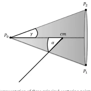
Evaluating the case of a conical warhead, three domi-nant points of scattering are usually considered. The first coincides with the tip of the cone, the others two corre-spond to the intersection between the base of the cone and the plane given by the radar LOS and the target symmetry axis. However, for warheads with fins, other points need to be considered, namely the tips of the fins. Therefore, assuming a simple conical warhead, the expression of the received signal is

srx(t)=

2

i=0

μi(t) exp

j2πf0

t− 2ρi(t)

c (6)

whereρi(t) depends on the micromotion matrix according to (4) and (5). In the case of conical warheads, the matrix

Tmis given by the product of three terms, namely

Tm= RcRsRn (7) where the matrices Rcand Rsdepend on conical movement and spinning, which together make up the precession, while

Rndepends on nutation. Since the matrices Rcand Rsare related to rotation movements, they can be obtained by the Rodrigues formula [2], [25]

Rc= I+E sin(ˆ ct)+Eˆ

2

(1−cos(ct))

Rs = I+E sin(ˆ st)+Eˆ

2

(1−cos(st)) (8)

where I is the identity matrix of dimension 3×3, c=

|wc|ands = |ws|, wherewcandws are the rotation an-gular velocity vectors of conical movement and spinning, respectively, while ˆEcand ˆEsrepresent the skew symmetric

matrixs [2] obtained by normalized vectorswcandws. In order to evaluate the matrix Rn, a new coordinate system (xn,yn,zn) has to be considered. The unit direc-tional vector that identifies the symmetry axis of the conical warhead with respect to the principal system ( ˆX,Y ,ˆ Zˆ) is defined as follows

ˆzt0 =Rt0a0 (9)

where a0=(0,0,1)T. Due to the precession, the

coordi-nates of target axis depend on time for its rotation during the conical motion, namely

ˆzt = RcRt0a0 (10) where ˆzt represents the unit directional vector at time in-stantt. Considering the cone axis oscillating in the plane given byOC(see Fig. 2) and ˆzt, the new reference system (xn,yn,zn) is chosen so thatxncoincides with the preces-sion axis while theznaxis is perpendicular to the oscillation plane, as shown in Fig. 2.

Therefore, the expressions of the three unit directional vectors of the system are

xn=

OC

OC, zn= OC׈zt

OC׈zt, yn=

xn×zn

xn×zn

.

Fig. 2. The reference system (xn, yn, zn).

Considering the three unit directional vectors (x,y,z) of

the system ( ˆX,Y ,ˆ Zˆ), the transition matrix An, which rep-resents the relationship between the previous and the new system, is given by

(xn,yn,zn)=(x,y,z) An. (12) Since the reference coordinates ( ˆX,Y ,ˆ Zˆ) are the natural coordinates, which means that (x,y,z) form a 3×3 iden-tity matrix, then matrix Anis obtained as follows

An=(xn,yn,zn) (13) from which it is clear that the transition matrix is orthonor-mal. Therefore, the position vector of a generic point in the new reference system at initial time instantt0is

rnp(t0)=(xnp(t0), ynp(t0), znp(t0))

T _{= A}−1

n rp(t0). (14)

Considering the case of a sinusoidal oscillation of the pre-cession angle, which is given byβ(t) (as shown in Fig. 2), then

β(t)=βnsin(ωnt)=βnsin(2π fnt) (15)

where fn and βn represent the frequency and maximum value of the oscillation, respectively. Since in the new ref-erence system the oscillation of the cone axis is a rotation around the znaxis, the position vector rnp(t) at the instant t is

rnp(t)= Bnrnp(t0)= BnA

−1

n rp(t0) (16)

where Bnis the Euler rotation matrix aroundznaxis given by

Bn=

⎡ ⎢ ⎣

cos(β) −sin(β) 0

sin(β) cos(β) 0

0 0 1

⎤ ⎥

⎦. (17)

The position vector in the natural coordinates system is given by

rt = Anrnt = AnBnA

−1

n rt0. (18)

Fig. 3. Representation of three principal scattering points of conical warhead.

TABLE I

Value of the Occlusion Functionμi(t) for the Three Principal Scattering PointsP0,P1, andP2With Respect to the Aspect Anglesα

α < γ γ≤α < π₂−γ ≤ π₂ ≤ π−γ

π

2−γ α <

π

2 α < π−γ ≤α≤π

μ0(α) 1 1 1 1 0

μ1(α) 1 1 1 1 1

μ2(α) 1 0 0 1 1

Finally, the nutation matrix Rncan be written as

Rn= AnBnA−1n . (19) The occlusion functionμi(t) depends only on the aspect angleα(t) and the semiangleγthat defines the cone shown in Fig. 3. The functions μi(t), withi=0,1,2, are eval-uated forα(t)∈[0, π] due to the symmetric shape of the target and to the specific micromovements exhibited by war-heads. Specifically, for the tip of the cone identified withP0,

the occlusion functionμi(t)=0 forα(t)≥π−γ, which means that in this interval occlusion occurs. For the scatter-ing pointP1, which is one of the points on the cone base at

minimum distance from the radar, occlusion never occurs, so the functionμi(t)=1 for all values ofα(t). On the other hand for the pointP2occlusion occurs whenα(t)∈[γ ,π₂].

The interval of occlusion for several scattering points are summarized in Table I.

Let us now consider the warheads with fins then the received signal can be modeled as follows:

srx(t)=

2

i=0

μi(t) exp

j2πf0

t−2ρit c

+

Nfin

a=1

μa(t) exp

j2πf0

t−2ρat

c (20)

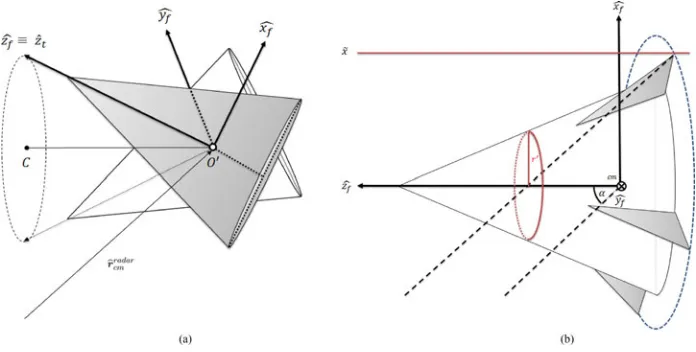
approx-Fig. 4. (a) Reference system (xf,yf,zf). (b) Representation of the threshold ˜x.

imation given the high frequency at which the radar system operates. Since the targets of interest are within the Fraun-hofer zone [2], the rays that strike the targets can be con-sidered as parallel. The occlusion of fins can only occur for values of the aspect angle such thatα(t)≥γfin, whereγfin

is the semiangle of an isosceles triangle whose height is equal to the height of the cone and the base is equal to the diameter of circumference drawn by rotating fins. There-fore, the functionμa(t)=1 whenα(t)∈

0, γf in

. In order to evaluateμa(t) forα(t)≥γf in, a new reference system (xf,yf,zf) has to be considered, as shown in Fig. 4(a). The reference system is chosen in order to have thezf axis coincident with the cone axis, whiley_f is perpendicular to the plane given by the radar LOS and the cone axis

zf =ˆzt, yf =

zf × rradarcm

zf × rradarcm

, xf =

y_f ×zf

y_f ×zf

.

(21) Since the reference system ( ˆX, Y ,ˆ Zˆ) is the natural coor-dinate system, the transition matrix Af is given by

Af =(xf,yf,zf). (22) The position vector of theath fin tip in the new system is given by

rfa =(xfa, yfa, zfa)

T _{= A}−1

f ra (23)

where ra is the position vector in the natural system. The value of occlusion function forα(t)≥γfin is calculated by

comparing the coordinatexfa with a suitable threshold as follows

μa(t)=

1 ifxfa <x˜ 0 ifxfa ≥x˜

. (24)

In order to evaluate the threshold ˜xit is necessary to calcu-late when the straight line joining the radar and tip of the fin becomes tangential to the cone surface [see Fig. 4(b)].

Considering the reference system (xf0,yf0, zf0) ob-tained moving the origin of system (xf,yf, zf) into center of cone bottom as shown in Fig. 5, the position vectors of

Fig. 5. Reference system (xf₀,yf₀,zf₀).

the fin tipOF, and of the radarOSare

OF =(R+Hf) cos(φ),(R+Hf) sin(φ),0

T

OS=−dsin(α),0, dcos(α)T (25)

where R is the bottom radius of the cone, Hf is the fin height, φ is the angle between the fin and xf0 axis, and where

α=tan−1

dsin(α)

dcos(α)+L

(26)

dd+Lcos(α) (27)

withαthe aspect angle,d= rradar_cm the distance between the radar and the mass center, andLthe distance between the mass center and the bottom center of the cone.

The conical surface is represented by the function:

f(xf0, yf0, zf0)=r

2₋

x_f2₀+y_f2₀

=R2

1− zf0 H

2

wherer=r(zf0) is the radius of the generic cone section given by

r(zf0)=R

1− zf0 H

(29)

whereH is the cone height. Considering the generic point of the coneP whose position vector is

OP =

rcos(ψ), rsin(ψ), H

1−r

R T

(30)

whereψ is the position angle with respect toxf0 axis, the lines fromPtoF andSare

P F =OP−OF =

rcos(ψ)−(R+Hf) cos(φ), r

sin(ψ)−(R+Hf) sin(φ), H

1− r

R

T

P S =OP−OS=

rcos(ψ)+dsin(α), rsin(ψ),

H

1− r

R

−dcos(α)

T

(31)

respectively. In order to evaluate the occlusion threshold, it is necessary to evaluate the angle φand ψ such thatP F

andP Sare both tangent to the conical surface as follows

⎧ ⎪ ⎪ ⎨ ⎪ ⎪ ⎩ ∂f ∂xf0

,_∂y∂f f0

,_∂z∂f f0

T

·P F =0

∂f ∂xf₀,

∂f ∂yf₀,

∂f ∂zf₀

T

·P S =0

(32)

where the components of gradient vector for a generic cone point are evaluated from (28) as

∂f ∂xf0

= −2xf0= −2r

_cos(ψ);

∂f ∂yf0

= −2yf0 = −2r

_sin(ψ);

∂f ∂zf0

= −2R2 H

1− zf0 H

= −2Rr H ;

(33)

with

xf0 =r

_{cos(ψ); y}

f0 =r

_{sin(ψ); z}

f0=H

1− r

R

.

(34) From (32) and (33) follows

⎧ ⎪ ⎪ ⎪ ⎪ ⎪ ⎪ ⎨ ⎪ ⎪ ⎪ ⎪ ⎪ ⎪ ⎩

(−2r)rcos2_(ψ)−(R+H

f) cos(ψ) cos(φ)

+rsin2(ψ)−(R+Hf) sin(ψ) sin(φ)−r+R

=0

(−2r)dsin(α) cos(ψ)+rcos2_(ψ)+rsin2_(ψ)

+R−r−Rd

_cos(α)

H

=0

(35)

Fig. 6. Example of threshold values ˜xas a function of aspect angle (α).

which leads to

⎧ ⎨ ⎩

cos(ψ−φ)= _R+R_H f cos(ψ)=

dcos(α)R

H −R

1

dsin(α)=

tan(γ) tan(α)−

R dsin(α)

.

∀r>0 (36)

Finally, the threshold is given by

˜

x=(Hf +R) cos(φ) (37)

where

φ=cos−1

tan(γ) tan(α)−

R dsin(α)

−cos−1

R R+Hf

.

(38) Fig. 6 shows how the threshold values varies as a function of aspect angle for the cone dimensionsH andRof 1 and 0.375 m, respectively, fin height Hf =0.200 m and at a distance of 150 km. It has to be pointed out that ˜xdepends on the distance between the target and radar, which makes this general model valid also for distances relatively small, e.g., in the case of an on-board radar of an interceptor.

B. Confusing Object

In the case of confusing objects, according to (2), the received signal is given by

srx(t)= Nd

i=0

μi(t) exp

j2πf0

t−2ρit

c (39)

whereNd in the number of scatterers. Since the confusing objects only wobble, and assuming for simplicity that the angular rotation vector is perpendicular to the plane given by the symmetry axis of the objects and the radar LOS, the matrix Tmis given by Rodrigues formula [2], [25]

Tm=Tr = I+E sin(ˆ rt)+Eˆ

2

(1−cos(rt)) (40)

where r = |wr| and wr is the angular rotation velocity vector, while ˆE is the skew symmetric matrix obtained by

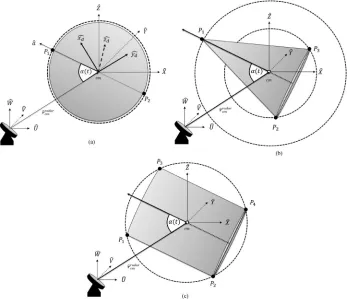
Fig. 7. Representation of the scattering points of confusing objects. (a) Sphere. (b) Cone. (c) Cylinder.

the symmetry axis of the object and the radar LOS and the sphere. In order to evaluate the phenomenon of occlusion for the spherical object, a new reference system (xd,yd, zd) is considered, as illustrated in Fig. 7(a). Assuming that the sphere axisad is the line passing through the two scatter-ers, the y_d axis is chosen so as to be parallel to the radar LOS, while the zd axis is perpendicular to the plane iden-tified by the radar LOS and the sphere axis, as illustrated in Fig. 7(a). Therefore, the unit directional vectors of the system are given by

y_d = r

radar

cm

rradar

cm

, zd =

ad×rradarcm

ad×rradarcm

, xd =

y_d× zd

y_d× zd

.

(41) Since the reference system ( ˆX, Y ,ˆ Zˆ) is the natural ref-erence system, the transition matrix Ad between the two system is

Ad =(xd,yd,zd). (42) The position vector of theith scattering point in the new reference system is given by

rdi =(xdi, ydi, zdi)

T ₌

A−_d1ri (43) where riis the position vector in the natural reference sys-tem. Furthermore, the occlusion for the scatterers occurs when the coordinateydi >0, so it follows

μi(t)=

1 ifydi ≤0 0 ifydi >0

. (44)

As for the warhead, three scatterers are considered for the conical object, namely the tip of the cone and the two on the base in proximity of the plane given by target symmetry axis and the radar LOS, as shown in Fig. 7(b). However, because of the different motion of the confusing object compared to the warhead, the occlusion of the three points is evaluated for values of the aspect angle which lays in [0,2π]. In particular,μi(t)=0 for the following:

1) P1whenα(t)∈[π −γ , π+γ];

2) P2whenα(t)∈

3π

2 ,2π−γ

;

3) P3whenα(t)∈

γ ,π₂.

Finally, for cylindrical objects four scattering points are considered: two for each base of the cylinder and on the plane given by target symmetry axis and the radar LOS. As for the conical object, the occlusion function for these points depends only on the aspect angle, specificallyμi(t)=0 for the following:

1) P1whenα(t)∈

π,3π

2

;

2) P2whenα(t)∈

3π

2 ,2π

;

3) P3whenα(t)∈ _π

2, π

;

4) P4whenα(t)∈

0,π

2

Fig. 8. Block diagram of the proposed algorithm.

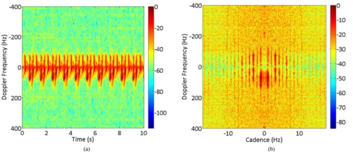
Fig. 9. Example of spectrogram and CVD obtained by a received signal from a cylindrical object. (a) Spectrogram. (b) CVD.

Fig. 7(c) shows the scattering points considered for a cylindrical object and their circular trajectory during its flight.

III. FEATURE EXTRACTION ALGORITHM

In this section, the algorithm to extract micro-Doppler-based features for the classification of ballistic targets is described. Fig. 8 shows a block diagram of the classification method outlining the common steps for the three different approaches proposed in this paper. The starting point of the proposed algorithm is the received signal ˜srx(n), with

n=0, ..., N, containing micro-Doppler components and comprising ofNsignal samples. The received signal has to be preprocessed before the evaluation of the micro-Doppler signature. The first block includes a notch filtering, down-sampling, and normalization (as required for the pZ-based method). The second step is the spectrogram computation of the preprocessed signal ˜srx(n)

χ(ν, k)=

N−1

n=0

˜

srx(n)wh(n−k) exp

−j2π νn N

, k=0, . . . , K−1 (45)

where ν is the normalized frequency and wh(·) is the smoothing window. The spectrogram is a TFD that allows the signal frequency time variations to be evaluated and it is chosen for its robustness with respect to the production of artefacts. In Fig. 9(a), the spectrogram obtained by a sig-nal scattered from a cylindrical object is shown. Observing Fig. 8, the next step consists in the extraction of the CVD, that is defined as the Fourier transform of the spectrogram along each frequency bin [5]:

(ν, ε)=

K−1

k=0

χ(ν, k) exp

−j2π εk K

(46)

whereε is known as the cadence frequency. The CVD is chosen because it offers the possibility of using, as discrim-inants, the cadence of each frequency component and the maximum Doppler shift, and because the CVD is more ro-bust than the spectrogram since it does not depend on the ini-tial phase of moving objects. In Fig. 9(b), the CVD obtained from the spectrogram given in Fig. 9(a) is shown, in which it is possible to see that the zero cadence component is fil-tered out. Finally, the CVD has to be processed to extract aQ-dimensional feature vector F =F0, F1, . . . , FQ−1

, which can identify unequivocally each class. The feature extraction block of Fig. 8 for the three different approaches will be described in the following sections. Before classifi-cation, the vector F is normalized as follows

˜

F= F−ηF

σF

(47)

where ηF and σF are the statistical mean and standard deviation of the vector F, respectively.

The classification performances of the extracted feature vectors are evaluated using thek-Nearest neighbor (kNN) classifier, modified in order to account for unknown class. In particular, letT be the training vectors set, for each class

van hypersphereSCMv(ζv) is considered, with center CMv and radiusζv. In the case in which the tested vector does not belong to any hypersphere, it is declared as unknown. The operation mode of this classifier is composed by three phases. In the first phase, the set N of nearest neighbor training vectors to the tested vector F is selected fromT as follows

N =!_F˜_{1, . . . ,F}˜_{k :∀i=1, . . . , k, F}˜_i−F

< min

˜

F∈{T−F˜1,...,F˜i−1}

_F˜ _{−F . (48)}

can assume an integer value in the range [0, V], whereV

is the number of possible classes. The value 0 is assigned when the tested vector does not belong to any hypersphere of the vectors inN, while the values [1, V] correspond to a specific class. Specifically,∀i=1, . . . , k, thei-labelιiis updated as follows

ιi=

0 F˜i−F> ζv

v otherwise (49)

wherevis the value corresponding to the belonging class of ˜

Fi. Finally, the (V +1)-dimensional score vector s is eval-uated, whose elements are the occurrences, normalized to

k, of the integers [0, . . . , V] in the vectorι. The estimation rule then may be implemented as follows:

ˆ

v=

arg max_vs if max(s)> 1₂

0 otherwise (50)

where 0 is the unknown class.

Assuming that the feature vectors of each class are dis-tributed uniformly around their mean vector, for all the Monte Carlo runs, the hypersphere radiusζv was chosen equal toσv

√

12/2, whereσv=tr (Cv) and Cvis the covari-ance matrix of the training vectors which belong to the class

v. The choice is made according to the statistical propri-eties of uniform distributions. In fact, for one-dimensional (1-D) uniform variables, the sum of mean and the prod-uct between the standard deviation and the factor√12/2 gives the maximum possible value of the distribution. The choice of akNN classifier is justified for its low computa-tional load and its capability of providing score values as an output. However, in general other classifiers with similar characteristics could also be selected. The selection of the best classifier is outside the scope of this paper.

A. ACVD-Based Feature Vector Approach

In the ACVD-based feature vector approach, seven fea-tures are computed from the ACVD. The starting point is the mean of the CVD along each cadence bin; the resulting 1-D function is then normalized to have a unit area. From the resulting function ˘(n), n=0, . . . , Nc−1, whereNc is the number of cadence bins, four statistical indices are extracted :

(1) Mean:

F0=

1

Nc Nc−1

n=0

˘

(n). (51)

(2) Standard deviation:

F1= " # # $ 1

Nc−1 Nc−1

n=0

%

˘

(n)− 1

Nc Nc−1

n=0 ˘

(n)

&2 . (52)

(3) Kurtosis:

F2= 1

Nc

'Nc−1 n=0

˘

(n)−_N1 c

'Nc−1 n=0 ˘(n)

4

() 1

Nc−1

'Nc−1 n=0

˘

(n)−_N1 c

'Nc−1 n=0 ˘(n)

2*4−3.

(53) (4) Skewness:

F3= 1

Nc

'Nc−1 n=0

˘

(n)−_N1 c

'Nc−1 n=0 ˘(n)

3

() 1

Nc−1

'Nc−1 n=0

˘

(n)− _N1 c

'Nc−1 n=0 ˘(n)

2*3.

(54)

Three other indices, specifically the peak sidelobe level (PSL) ratio and two different definitions of the integrated sidelobe level (ISL) ratio, are computed from the normal-ized autocorrelation of the sequence ˘(n), C˘(m), m=

0, . . . , M−1. Specifically

F4=PSL=max

m

C˘(m) C˘(0)

(55)

while the latter are

F5=ISL1 = 'M−1

m=1 C˘(m)

C˘(0)

(56)

and

F6=ISL2 = 'M−1

m=1 C˘(m)

2 C˘(0)

(57)

respectively.

B. Pseudo-Zernike-Based Feature Vector Approach The pZ moments of orderr and repetitionl of an im-age I(x, y), introduced in [19], are geometric moments computed as the projection of the image on a basis of 2-D-polynomials which are defined on the unit circle. They are calculated as

ζr,l =

r+1

π + 2π

0 + 1

0

W_r,l∗ (ρ, θ)I(ρcosθ, ρsinθ)ρdρdθ

(58) where

Wr,l(ρ, θ)= r−|l|

h=0

ρr−h₍₋₁₎h_(2r+1−h)!

h! (r+ |l| +1−h)! (r− |l| −h)!e j lθ_,

with ρ≤1. (59)

The moments have several properties, among which are that they are independent, since the pZ polynomials are orthogonal on the unit circle, and their modulus is rotational invariant.

whosezth element is

Fz=ζr,l (60)

wherer=l =0, . . . , K−1 andz=0, . . . ,(k+1)2−1. Since the pZ moments are defined on the unit circle, the support of the spectrogram, hence that of the CVD, has to be chosen to be a unit square so that it can be inscribed in the unit circle [5], [18].

C. Gabor Filter Based Feature Vector Approach

The 2-D Gabor function is the product of a complex exponential representing a sinusoidal plane wave and an elliptical 2-D Gaussian bell. Its analytical expression in the spatial domain, which can be normalized to have a compact form [22], [24], is

ψ(x, y)= f

2

π γ ηe −f2

γ2x 2

+f2 η2y

2

ej2πf x (61)

with

x=xcos(θ)+ysin(θ) and y= −xsin(θ)+ycos(θ) (62) wheref is the central spatial frequency,θis the anticlock-wise angle between the direction of the plain wave and the ˆx-axis, γ is the spatial width of the filter along the plane wave, andηis the spatial width perpendicular to the wave. Therefore, the sharpness of the filter is controlled on the major and minor axes byηandγ. The normalized expression of the Gabor function in the Fourier domain is [22]

(u, v)=e−π 2 f2

γ2_(u−f)2

+η2_v2

(63)

where

u=ucos(θ)+vsin(θ) and v= −usin(θ)+vcos(θ).

(64) In the proposed technique, as in the pZ moments based approach, the magnitude of the CVD, scaled to fit the unit square, is normalized to obtain a matrix whose values be-longs to the set [0,1] as follows

¯

(ν, ε)= (ν, ε)−minν,ε(ν, ε)

maxν,ε(ν, ε)−minν,ε(ν, ε). (65) Then, the resulting matrix ¯(ν, ε) is filtered with a bank of Gabor filters whose impulse responses are

ψm,l(x, y)=

f_l2 π γ ηe

−

f_l2 γ2x

2

+f_l2 η2y

2

ej2πflx ₍₆₆₎

with

x=xcos(θm)+ysin(θm) and

y= −xsin(θm)+ycos(θm) (67)

for variousflandθm,l=0, . . . , L−1,m=0, . . . , M− 1, whereLandMare the numbers of selected spatial central frequencies and orientation angles, respectively. The choice of theflandθmdepends on the specific application and on the worst case image to represent with the moments. The selection of these parameters has to be conducted in order

to get an accurate representation of the image under test. In fact, since by varyingθm, the harmonic response of the filter moves on a circumference, whose radius isfl, it is possible to extract local characteristics in the Fourier domain by choosing a set of values for the two parameters [21]. The value of each pixel of the output image is given by the convolution product of the Gabor function and the input image ¯(ν, ε) as

gl,m(ν, ε;fl, θm)=ψl,m(ν, ε;fl, θm)∗¯(ν, ε)

= + _∞

−∞ + _∞

−∞ψl,m(ν−ντ, ε−ετ;fl, θm) ¯(ντ, ετ)dντdετ

(68)

with l=0, . . . , L−1 and m=0, . . . , M−1, where L

and M are the numbers of central frequency and orien-tation angles, respectively. Finally, the outputs of the filters are processed to extract the feature vector used to classify the targets. In particular, a feature is extracted from the out-put image of each filter by adding up the values of all pixels [21], as

Fq =gl,m = Nν−1

ν Nε−1

ε

|gl,m(ν, ε;fl, θm)| (69)

where q=mL+l, with l=0, . . . , L−1 and m=

0, . . . , M−1, Nν and Nε are the dimensions of the im-age ¯along both axis.

IV. PERFORMANCE ANALYSIS

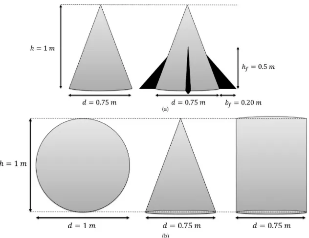
In this section, the proposed model is tested with both simulated data and real data acquired from replicas of the targets of interest. The targets are divided in two classes, which are warhead and confusing object. Moreover, both of them are divided in subclasses, which are associated to a particular type of target. Specifically, the warhead class is composed by two subclasses: cone and cone with triangular fins at the base, which are replicas of warhead without and with fins, respectively. Confusing object class, in contrast, is divided in three subclasses: sphere, cone, and cylinder.

The conical warhead has a diameterdof 0.75 m and a heighthof 1 m, while the fin’s basebf is 0.20 m and the heighthfis 0.50 m, as shown in Fig. 10(a). The sizes of the confusing objects are usually comparable with the dimen-sions of the warheads in order to confuse the antimissile radar system. Therefore, both the cylindrical and conical objects are chosen to have a diameter and a height equal to 0.75 and 1 m, respectively, while the sphere diameter is 1 m, as shown in Fig. 10(b).

In order to analyze the performance of the proposed algorithm, three figures of merit are considered, which are the Probability of correct Classification (PC), the

Proba-bility of correct Recognition (PR), and the Probability of

Fig. 10. Dimensions of the replicas of the targets of interest. (a) Warheads. (b) Confusing objects.

classifier does not make a decision and the total number of analyzed objects. A Monte Carlo approach is used in or-der to calculate the mean of the three figures of merit over several cases. Specifically, the means are evaluated over 50 different Monte Carlo runs in which all the available signals are divided randomly into training or testing sets with 70% used for training and 30% for testing. Thekvalue of classi-fier has to be chosen greater than 1 in order to consider the

unknown class; especially it is set to 3 for the ACVD and

Ga-bor filter based methods, while it is 5 for the pZ based one. These two specific values ofkare selected as they resulted to provide the best performance for the three approaches.

The performance is shown for varying the signal to noise power ratio (SNR) and observation time, which is either 10, 5, or 2 s. Moreover, for both the pZ and the Gabor filter methods, the dimension of the feature vector is also varied. The spectrogram is computed using a Hamming window with 75% overlap. The number of points for the DFT computation Nbin is fixed for the ACVD approach,

whereas it is adaptively evaluated for the pZ and the Gabor filter methods, in order to obtain a square representation of the spectrogram. Specifically, in these casesNbin is given

by

Nbin= ,

N−Woverlap

W(1−overlap)

-(70)

where N is the number of signal samples, ·represents the smaller integer greater than or equal to the argument, and overlap is the percentage of overlap expressed in the interval [0,1]. Finally, it is assumed that the effect of the principal translation motion of the targets is compensated before the signals are processed.

A. Simulated Data

The database for simulated data is composed of 105 realizations of the received signal for each target of interest, obtained by considering 15 signals for 7 different values of the elevation angleαEas follows:

αE=ε15◦ with ε=0, ...,6 (71)

while the azimuth angleαAis set to 0◦. The initial phase of the micromotions is taken randomly in uniform distribution [0,2π] and an additive white Gaussian noise is added to each simulation.

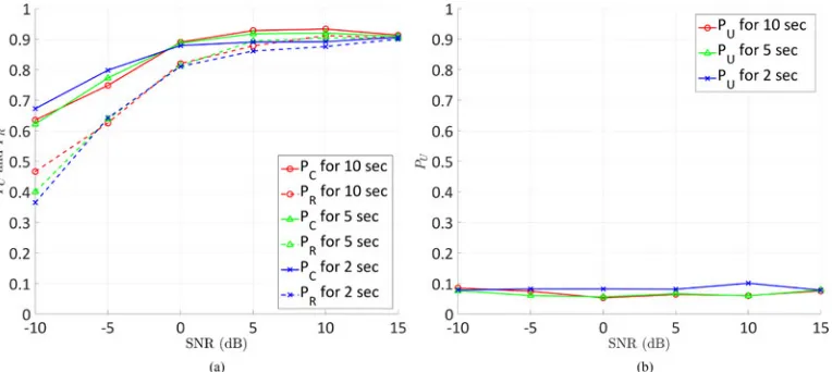
Fig. 11(a) showsPCandPRfor the ACVD-based feature vector approach. It is clear that both of them increase as the SNR increases, while showing a slight difference as the signal’s duration varies. Moreover,PC andPRbecome similar as the noise decreases. Observing Fig. 11(b), which showsPU, it is noted that it is almost constant at about 0.1, for all the values of SNR and signal duration considered. Defining the probability of misclassificationPMas

PM =1−PC−PU (72)

and sincePC is slightly greater than 0.9 for SNR greater than 0 dB, it is clear thatPMdecreases as the SNR increases, becoming smaller than 10−2.

Fig. 11. Performance of the ACVD-based feature vector approach for simulated data on varying the signal’s duration and the SNR. (a)PCandPR. (b)PU.

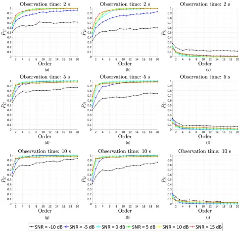
reach probabilities of about 0.99 for order greater than 8. Fig. 12(c), (f), and (i) represent the performance in terms of

PU. It is possible to observe that, for SNR greater than−5 dB, the performance generally improves as both signal du-ration and moments order increase. For observation times of 5 and 2 s,PUis smaller than 0.1, for orders greater than 4 and for all the noise levels; in contrast, for duration equal to 10 s and for SNR of−10 dB,PU is about 0.1, while for lower noise levels PU becomes smaller than 10−2 as the order increases.

Fig. 13 showsPC,PR, andPU for the Gabor filter ap-proach. For this approach, the dimension of feature vector corresponds to the number of filters, which depends on the orientation angular stepθstep. Recall that the number of

features,Qis given by

Q=L ,

π/2

θstep

-+1

(73)

where θstep is the orientation angular step and L in the

number of central frequencies. The latter was fixed at four values; 0.5, 1, 1.5, and 2. The value of θstep was set to be

an integer in the interval [3◦,10◦]. In this way, an analysis on varying the density of the considered positions of the harmonic response on each circumference with radius equal tofl is conducted. The values of the orientation angle,θm, is given by

θm=m θstep (74)

withm=0, . . . , M−1 and where

M= ,

π/2

θstep

-. (75)

From (74) and (75), it is important outlining that the features are extracted moving the harmonic response of the filter considering only the first quadrant, due to the symmetry of the expected image for this application.

Fig. 13(a), (b), (d), (e), (g), and (h) show thatPC and

PR are approximately equal, and for a signal duration of 2 s, they increase quickly, becoming greater than 0.98 for

SNR greater than −5 dB. For signal durations of 5 and 10 s, instead,PC andPR are greater than 0.98 for all the considered values of SNR andQ. As shown in Fig. 13(c), (f), and (i), PU is always smaller than 0.05. Finally it is noted that the performance does not change significantly when varying the feature vector dimension.

B. Real Data

Fig. 14 shows the experiment setup used to acquire the real data. The real data was acquired from signals scattered from targets of interest with a representative radar. Partic-ularly, ten acquisitions of 10 s were made for each target and for each of the possible nine pair of azimuth and ele-vation angles formed using three values for both of them, namely [0◦; 45◦; 90◦]. The acquisition of 10 s has been also split into segments of 5 and 2 s for the analysis on the signal duration. The parameters of the micromotions were chosen as for simulated data, and the precession, nutation, and wobbling were simulated using an ST robotic manip-ulator R-17 and an added rotor [26], for both warheads and confusing objects. As it can be noted from pictures in Fig. 14, which shows the experiment setup, the robotic arm is wrapped with anechoic material such that acquired signals contain only the micro-Doppler from the targets. The rotor is attached to the wrist of the robotic arm and it is used to simulate the warhead spinning and confusing objects wobbling. Moreover, by means of a synchronized and perturbed rotation of robotic arm and the wrist, the conical movement and nutation are simulated. It has to be underlined that the trajectory of ballistic targets is not taken into account in the experiment considering that the princi-pal movement of the object is compensated. In this way, the classification is based only on the micromotions of targets of interest.

Fig. 12. Performance of the pZ-based feature vector approach for simulated data; the analysis is conducted on varying the order, the signal’s duration, and the SNR. (a)PC. (b)PR. (c)PU. (d)PC. (e)PR. (f)PU(g)PC. (h)PR. (i)PU.

Moreover, it is pointed out that the main differences be-tween the simulated and the real case are due to the fact that in the presented simulation model the RCS of the scat-ters is not taken into account, and the initial phase of the micromotions is random in both two cases. The perfor-mance is evaluated by varying the signal duration and the SNR, as for the simulated data. In addition, assuming that the noise for the acquired signals in a controlled environ-ment is negligible, the analysis on the SNR was conducted by adding white Gaussian noise to the real data. Finally before processing, the received signals are down-sampled by a factor of 10.

Fig. 16(a) showsPCandPR, while Fig. 16(b) shows the

PU for the ACVD-based method. The performance trend

obtained in the previous section for the simulated data is confirmed by the real data. In fact, bothPCandPRincrease as the SNR increases; however, the effect of changing the observation time is more evident in this case. Moreover, the gap between the two figures of merit decreases as both the duration of the signals time and the SNR increase. Observ-ing Fig. 16(b),PUis almost constant for all analyzed cases and it is smaller than 0.1.

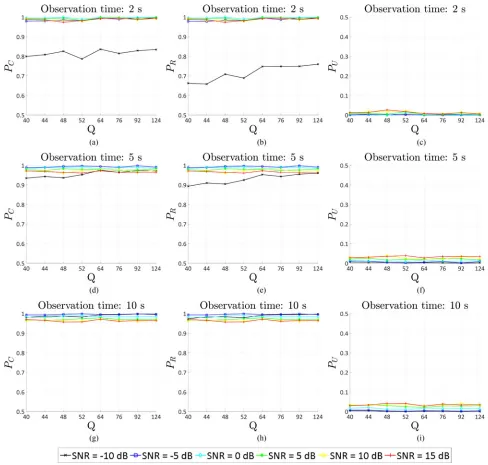
ob-Fig. 13. Performance of the Gabor Filter based feature vector approach for simulated data; the analysis is conducted on varying the number of featuresQ, the signal’s duration, and the SNR. (a)PC. (b)PR. (c)PU. (d)PC. (e)PR. (f)PU. (g)PC. (h)PR. (i)PU.

serving Fig. 17(c), (f), and (i), it is clear thatPU increases as the observation time increases. The reason of this be-havior seems likely to be due to the choice of the k-means classifier. In fact, for greater values of the signal duration, the feature vectors of a given class occupy a smaller re-gion in the multidimensional space: then, it is more likely that a feature vector under test is not close enough to be classified as belonging to the correct class. A different clas-sifier, less dependent on distances in the multidimensional space might produce different results. Moreover, PU de-creases as the SNR and the moments order inde-creases. The gap betweenPC andPRbecomes smaller as the moments order increases. However, unlike the performance obtained

on simulated data, the maximum value reached by the two probabilities is around 0.90.

Fig. 18 shows the performance of the Gabor filter based method. Observing Fig. 18(a), (b), (d), (e), (g), and (h), it is clear that both PC andPR increase as the SNR and observation time increase. In particular, for signal duration of 5 s, both PC and PR are greater than 0.98 for SNR greater than −10 dB; for duration equal to 10 s, instead,

Fig. 14. Experiment setup.

Fig. 15. Example of spectrogram obtained by a received signal from a warhead with fins. (a) Simulated data. (b) Real data.

Fig. 16. Performance of the ACVD-based feature vector approach for real data on varying the signal duration and the SNR. (a)PCandPR. (b)PU.

the results it is clear that higher is the SNR then higher are the performance.

C. Performance in Presence of the Booster

The performance with real data was evaluated also in the case in which the received signal was scattered from an additional object different from warheads and confusing

Fig. 17. Performance of the pZ-based feature vector approach for real data; the analysis is conducted on varying the moments order, the signal duration and the SNR. (a)PC. (b)PR. (c)PU. (d)PC. (e)PR. (f)PU. (g)PC. (h)PR. (i)PU.

is assumed that the booster has a cylindrical shape, whose diameter and height are 0.75 and 5 m, respectively, with triangular fins, whose base is 0.50 m and height is 1 m; the wobbling velocity is one fifteenth of that of the confusing objects.

This analysis is conducted by training the classifier with feature vectors belonging to either warhead class or confus-ing object class, and then by testconfus-ing it on the booster feature vector. Moreover, the performance is evaluated in terms of

PU, as defined above, and probability of misclassification

(Error) as a Warhead (PeW), determined by the ratio of the number of times in which the booster is classified as a warhead and the total number of tests. Note, in this spe-cific case, classifying the booster as unknown represents the correct classification as there is no specific booster class.

Fig. 20 shows PU and PeW obtained by the ACVD-based algorithm as the signal duration and the SNR are varied. From Fig. 20 it is observed that even ifPUincreases and, consequently, PeW decreases as the signal duration

increases,PeWremains greater thanPU. Moreover, the per-formance does not change significantly on varying the SNR. Results obtained by using the pZ-Based approach are shown in Fig. 21. Observing the figure it is clear that the probability of classifying the booster as unknown increases as the order grows up to 4, independently of the observation length, where the maximum value is reached, and it is above 0.80 for SNR equal to 0 and 5 dB. Considering orders greater than 4,PU remains constant for positive values of SNR, while it significantly decreases for SNR smaller than 0 dB. However, for moments order of about 20,PUgrows as the SNR increases. It is noticed thatPeW decreases as the observation time increases for negative value of SNR, while it increases for SNR greater than 0 dB. However, the best results are obtained for positive values of the SNR and for signal duration of 2 and 5 s, reaching probabilities of error smaller than 0.20.

Fig. 18. Performance of the Gabor Filter based feature vector approach for real data; the analysis is conducted on varying the number of featuresQ, the signal duration and the SNR. (a)PC. (b)PR. (c)PU. (d)PC. (e)PR. (f)PU. (g)PC. (h)PR. (i)PU.

Fig. 20. Performance of the ACVD-based feature vector approach for real unknown data (booster); the analysis is conducted on varying the

number of featuresQ, the signal duration and the SNR.

Fig. 21. Performance of the pZ-based feature vector approach for real unknown data (booster); the analysis is conducted on varying the moments order, the signal duration and the SNR. (a)PU. (b)PeW. (c)

PU. (d)PeW. (e)PU. (f)PeW.

deduce that the performance improves as the signal duration and the SNR increase. In particular, the performance for the signal duration of 2 s is not useful becausePeW is always greater thanPU. However, for observation time of 5 sPU becomes greater thanPeW from SNR greater than−10 dB reaching about 0.90 for highest values of SNR. Finally, for signal duration equal to 10 s,PUis constantly greater than 0.90 independently of the values of the SNR andQ; on the other hand,PeW is smaller than 10−2for values of the SNR greater than 0 dB.

Consequently it is clear that in the case of classifica-tion of unknown objects which are not used to train the classifier, such as the booster, the ACVD-based approach

Fig. 22. Performance of the Gabor Filter based feature vector approach for real unknown data (booster); the analysis is conducted on varying the number of featuresQ, the signal duration and the SNR. (a)PU. (b)PeW.

(c)PU. (d)PeW. (e)PU. (f)PeW.

does not guarantee satisfactory performance. The pZ-based approach is able to give good performance for small signal duration and for high SNR. Alternatively the Gabor filter approach provided the optimum results for an observation time of 5 s, for SNR greater than−10 dB, and of 10 s, independently of the noise levels.

CONCLUSION

been conducted in order to test the presented methods also in the case in which the feature vector under test does not belong to one of the classes of interest, such as the booster separated from warhead. Even in this case the results have shown that for a sufficient observation time, the framework is able to recognize the unknown target. Future work will involve a study of the best micro-Doppler features for bal-listic target classification in terms of computational cost and reliability. A new model based classification algorithm will be investigated that uses the proposed mathematical model in this paper.

ACKNOWLEDGMENT

The data which underpin this paper is subject to a con-fidentiality agreement with one of the collaborators—as such the data cannot be made openly available. Enquiries about this restriction can be submitted to [email protected] in the first instance.

REFERENCES [1] G. L. Silberman

Parametric classification techniques for theater ballistic missile defense

In Proc. Johns Hopkins Apl. Tech. Dig., 1998, vol. 19, no. 3, pp. 323–339.

[2] G. Hongwei, X. Lianggui, W. Shuliang, and K. Yong

Micro-Doppler signature extraction from ballistic target with micro-motions

IEEE Trans. Aerosp. Electron. Syst., vol. 46, no. 4, pp. 1969–

1982, Oct. 2010.

[3] L. Liu, D. McLernon, M. Ghogho, W. Hu, and J. Huang Ballistic missile detection via micro-Doppler frequency esti-mation from radar return

Digit. Signal Process., vol. 22, no. 1, pp. 87–95, 2012.

[4] V. Chen, F. Li, S. Ho, and H. Wechsler

Micro-Doppler effect in radar: Phenomenon, model, and simu-lation study

IEEE Trans. Aerosp. Electron. Syst., vol. 42, no. 1, pp. 2–21,

Jan. 2006.

[5] C. Clemente, L. Pallotta, I. Proudler, A. De Maio, J. Soraghan, and A. Farina

Pseudo-Zernike-based multi-pass automatic target recognition from multi-channel synthetic aperture radar

IET Radar, Sonar Navig., vol. 9, no. 4, pp. 457–466, 2015.

[6] F. Fioranelli, M. Ritchie, and H. Griffiths

Multistatic human micro-Doppler classification of armed/unarmed personnel

IET Radar, Sonar Navig., vol. 9, no. 7, pp. 857–865, 2015.

[7] L. Du, B. Wang, Y. Li, and H. Liu

Robust classification scheme for airplane targets with low res-olution radar based on EMD-clean feature extraction method

IEEE Sensors J., vol. 13, no. 12, pp. 4648–4662, Dec. 2013.

[8] F. Fioranelli, M. Ritchie, and H. Griffiths

Analysis of polarimetric multistatic human micro-Doppler clas-sification of armed/unarmed personnel

In Proc. IEEE Radar Conf., May 2015, pp. 0432–0437. [9] S. Bjorklund, H. Petersson, A. Nezirovic, M. Guldogan, and F.

Gustafsson

Millimeter-wave radar micro-Doppler signatures of human mo-tion

In Proc. 2011 Int. Radar Symp., Sep. 2011, pp. 167–174. [10] F. Fioranelli, M. Ritchie, and H. Griffiths

Classification of unarmed/armed personnel using the netRAD multistatic radar for micro-Doppler and singular value

decom-position features

IEEE Geosci. Remote Sens. Lett., vol. 12, no. 9, pp. 1933–1937,

Sep. 2015.

[11] P. Molchanov, K. Egiazarian, J. Astola, A. Totsky, S. Leshchenko, and M. Jarabo-Amores

Classification of aircraft using micro-Doppler bicoherence-based features

IEEE Trans. Aerosp. Electron. Syst., vol. 50, no. 2, pp. 1455–

1467, Apr. 2014.

[12] C. Hornsteiner and J. Detlefsen

Extraction of features related to human gait using a continuous-wave radar

In Proc. 2008 German Microw. Conf., Mar. 2008, pp. 1–3. [13] L. Liu, M. Popescu, M. Skubic, M. Rantz, T. Yardibi, and P.

Cud-dihy

Automatic fall detection based on Doppler radar motion signa-ture

In Proc. 2011 5th Int. Conf. Pervasive Comput. Technol.

Health-care, May 2011, pp. 222–225.

[14] I. Bilik, J. Tabrikian, and A. Cohen

Target classification using Gaussian mixture model for ground surveillance Doppler radar

In Proc. 2005 IEEE Int. Radar Conf., May 2005, pp. 910–915. [15] A. Ghaleb, L. Vignaud, and J. Nicolas

Micro-Doppler analysis of wheels and pedestrians in ISAR imaging

IET Signal Process., vol. 2, no. 3, pp. 301–311, Sep. 2008.

[16] S. Bjorklund, T. Johansson, and H. Petersson

Evaluation of a micro-Doppler classification method on MM-wave data

In Proc. 2012 IEEE Radar Conf., May 2012, pp. 0934–0939. [17] C. Clemente, A. Balleri, K. Woodbridge, and J. Soraghan

Developments in target micro-Doppler signatures analysis: Radar imaging, ultrasound and through-the-wall radar

EURASIP J. Adv. Signal Process., vol. 2013, no. 1, pp. 47–64,

2013.

[18] C. Clemente, L. Pallotta, A. De Maio, J. Soraghan, and A. Farina A novel algorithm for radar classification based on Doppler characteristics exploiting orthogonal pseudo-Zernike polyno-mials

IEEE Trans. Aerosp. Electron. Syst., vol. 51, no. 1, pp. 417–430,

Jan. 2015. [19] A. Bhatia and E. Wolf

On the circle polynomials of Zernike and related orthogonal sets

In Math. Proc. Cambridge Philosoph. Soc., 1954, vol. 50, no. 1, pp. 40–48.

[20] M. R. Teague

Image analysis via the general theory of moments∗

J. Opt. Soc. Amer., vol. 70, no. 8, pp. 920–930, Aug. 1980.

[21] A. R. Persico, C. Clemente, C. V. Ilioudis, D. Gaglione, J. Cao, and J. Soraghan

Micro-Doppler based recognition of ballistic targets using 2-d Gabor filters

In Proc. Sensor Signal Process. Defence Conf., Sep. 2015, pp. 1–5.

[22] J.-K. Kamarainen, V. Kyrki, and H. Kalviainen

Invariance properties of Gabor filter-based features-overview and applications

IEEE Trans. Image Process., vol. 15, no. 5, pp. 1088–1099,

May 2006.

[23] N. Mittal, D. Mital, and K. L. Chan

Features for texture segmentation using Gabor filters In Proc. 1999 7th Int. Conf. Image Process. Appl., Jul. 1999, vol. 1, pp. 353–357.

[24] J. Ilonen, J.-K. Kamarainen, and H. Kalviainen Fast extraction of multi-resolution Gabor features