Rochester Institute of Technology
RIT Scholar Works
Theses
Thesis/Dissertation Collections
3-1-2013
Investigation of the intermediate and high end
initial mass function as probed by near-infrared
selected stellar clusters
Christine Trombley
Follow this and additional works at:
http://scholarworks.rit.edu/theses
This Dissertation is brought to you for free and open access by the Thesis/Dissertation Collections at RIT Scholar Works. It has been accepted for inclusion in Theses by an authorized administrator of RIT Scholar Works. For more information, please [email protected].
Recommended Citation
i
INVESTIGATION OF THE INTERMEDIATE AND HIGH END INITIAL
MASS FUNCTION AS PROBED BY NEAR-INFRARED SELECTED
STELLAR CLUSTERS
By
Christine M. Trombley
A dissertation submitted in partial fulfillment of the requirements for the degree of Ph.D. in Astrophysical Sciences and Technology, in the
College of Science, Rochester Institute of Technology
March 2013
Approved by ________________________________________________________________ Prof. Andrew Robinson Date
i
ASTROPHYSICAL SCIENCES AND TECHNOLOGY COLLEGE OF SCIENCE
ROCHESTER INSTITUTE OF TECHNOLOGY ROCHESTER, NEW YORK
CERTIFICATE OF APPROVAL
Ph.D. DEGREE DISSERTATION
The Ph.D. Degree Dissertation of Christine M. Trombley has been examined and approved by the dissertation committee as satisfactory for
the dissertation requirement for the Ph.D. degree in Astrophysical Sciences and Technology.
ii
Dr. Karl Hirschman, Committee Chair
Dr. Judith L. Pipher
Dr. Michael Richmond
i
Abstract
ii
Contents
Abstract ... i
Contents ... ii
1. Introduction ... 1
1.1. The Initial Mass Function ... 2
1.1.1. Variations ... 7
1.1.2. Stellar Evolution Models: Past and Present ... 7
1.1.3. Method ... 8
1.1.4. Utilizing the IMF ... 10
1.2. Upper Mass Cut Off ... 11
1.3. Young Massive Clusters and Candidate Clusters ... 14
2. Observations ... 17
2.1. Sample of Cluster Candidates ... 17
2.2. Spizter/IRAC Imaging: Reduction and Photometry ... 17
2.3. HST/NIC3 Imaging: Reduction and Photometry ... 21
2.4. VLT/ISAAC Spectroscopy: Observations and Reduction ... 24
2.5. IRTF/SpeX Spectroscsopy: Observations and Reduction ... 25
2.6. Keck II/NIRC2 Imaging and Slitless Spectroscopy: Observations and Reduction ... 28
2.6.1. Laser Guide Star Adaptive Optics Imaging ... 28
2.6.2. Slitless Spectroscopy... 32
2.7. Chandra/ACIS: Reduction ... 37
2.8. VLT/MAD Imaging: Photometry in the core of R136 ... 37
3. Data Analysis ... 43
3.1. Mercer 5 ... 43
3.1.1. NIR Imaging ... 43
3.1.2. Slitless Spectroscopy... 44
iii
3.1.4. Mass, Age, and Distance ... 48
3.1.5. X-ray Source ... 51
3.1.6. Summary ... 52
3.2. Mercer 14 ... 52
3.2.1. Summary ... 54
3.3. Mercer 17 ... 54
3.3.1. Stellar Content ... 55
3.3.2. Summary ... 58
3.4. Mercer 20 ... 58
3.4.1. Stellar Content ... 58
3.4.2. Age, Reddening, Distance, Mass ... 65
3.4.3. Summary ... 66
3.5. Mercer 23 ... 66
3.5.1. Stellar Content ... 67
3.5.2. Age, Reddening, Distance, Mass ... 73
3.5.3. Summary ... 73
3.6. Mercer 30 ... 73
3.6.1. Stellar Content ... 74
3.6.2. Age, Reddening, Distance, Mass ... 80
3.6.3. Summary ... 81
3.7. Mercer 70 ... 81
3.7.1. Stellar Content ... 81
3.7.2. Age, Reddening, Distance, Mass ... 88
3.7.3. Summary ... 89
3.8. Mercer 81 ... 89
3.8.1. Stellar Content ... 90
iv
3.8.3. X-ray Properties ... 95
3.8.4. Summary ... 96
3.9. Danks 1 & Danks 2 ... 96
3.9.1. Stellar Content ... 96
3.9.2. Age, Distance, Mass... 98
3.9.3. X-ray Properties ... 99
3.9.4. Summary ... 102
3.10. [BDS2003] 66 ... 102
3.10.1. Stellar Content ... 103
3.10.2. Age, Reddening, Distance, Mass ... 109
3.10.3. Summary ... 109
3.11. [DB2001] Cl 20 ... 109
3.11.1. Stellar Content ... 109
3.11.2. Age, Reddening, Distance, Mass ... 115
3.11.3. Summary ... 115
3.12. [DB2001] Cl 9 ... 115
3.12.1. Stellar Content ... 116
3.12.2. Age, Reddening, Distance, Mass ... 125
3.12.3. Summary ... 125
3.13. [BDS2003] 52 ... 125
3.13.1. Stellar Content ... 128
3.13.2. Age, Reddening, Distance, Mass ... 134
3.13.3. X-ray & Radio Observations ... 134
3.13.4. Summary ... 138
4. Error Analysis ... 139
4.1. Distance... 139
v
4.3. IMF Simulations: Expectations vs Reality ... 141
4.3.1. Influence of IMF Form: Kroupa vs Salpeter ... 145
5. IMF Analysis ... 146
5.1. CMD decontamination ... 146
5.2. Conversion to K-band Luminosity function ... 148
5.3. Stellar Evolutiona Models ... 148
5.4. Construction of IMF ... 152
5.5. Slope Measurement Limits and Method ... 154
6. Results and Discussion ... 155
6.1. IMF Slope: Individual Results ... 156
6.1.1. Mercer 20 ... 156
6.1.2. Mercer 23 ... 161
6.1.3. Mercer 30 ... 162
6.1.4. Mercer 70 ... 163
6.1.5. Mercer 81 ... 165
6.1.6. Danks 1 ... 166
6.1.7. Danks 2 ... 167
6.1.8. The curious case of R136 ... 168
6.2. IMF Slope: Sample as a Whole ... 172
6.3. No Evidence for an Upper Mass Cut-off ... 176
6.4. Dynamical Considerations ... 177
7. Conclusions ... 181
7.1. The Slope Of the IMF ... 182
7.1.1. R136 ... 183
7.2. Upper Mass Cut-Off ... 183
8. Future Work ... 184
vi
8.2. Investigation of Mass Segregation ... 185
8.3. X-ray follow-up ... 186
8.4. FS CMa Stars ... 186
8.5. DB9 and the Surrounding Medium ... 187
8.6. Modeling and Spectra ... 187
8.7. R136 ... 188
9. References ... 189
10. Appendix A: HST/NIC3 Images ... 199
11. Appendix B: WISE Images ... 213
1
1.
Introduction
While not the primary source of mass in the universe, stars are the dominant source of visible light. Though the majority are unresolved, stars populate the galaxies observed by astronomers in the local and high-redshift universe. Stars are “building blocks” of galaxies. They form in clusters (Lada & Lada 2003) and disperse into the galactic field. Some star formation sites produce tightly bound clusters, such as the young super-star clusters observed in interacting galaxies (e.g. the Antennae, Whitmore et al. 1999). These super star clusters are thought to be modern precursors to old globular clusters. In external galaxies, individual stars cannot be resolved, requiring a study of the integrated light properties in order to fully understand these star-forming regions. These unresolved stellar populations must be modeled using population synthesis techniques, which in turn require basic assumptions regarding age (or age range), metallicity, and stellar mass distribution. While age and metallicity can be derived from integrated spectra, no method to derive a mass distribution based solely on integrated properties exists.
The frequency distribution of stellar masses, dN/dlogM (where dN in the number of stars in a given mass range dlogM), in local, resolved populations is often described as a log-log power law, ξ(M) proportional to M-α. This distribution is known as the initial mass function (IMF). Practically speaking, the IMF represents the inferred mass distribution of stars in a star formation event. The initial distribution of mass in a star forming event is rarely observed, rather the present-day distribution is observed and mapped back to an initial distribution. The IMF appears to be an essentially universal power law above 1 solar mass (M) (Salpeter 1955, Kroupa 2002, Massey 2003, Bastian et al. 2010). The IMF plays a large role in extragalactic astrophysics, as the functional form of the IMF is required for calculating the expected baryonic mass-to-light ratio in an unresolved population. The choice of IMF and star formation history is also used to predict the number of stellar remnants present in a given population, e.g. globular clusters, the Galactic center region.
Massive star formation remains a theoretical challenge (Zinnecker & Yorke 2007) that can be probed by the high mass end of the IMF. If the properties of the star-forming environment are essential in determining the resulting mass spectrum, then the IMF should display some trend with environmental parameter(s). However, this is in direct contradiction to observations of a putative universal power law distribution. Comparing the slope of the IMF among multiple young massive clusters directly tests the claimed universality of the slope. Any significant deviations from the average IMF slope can then be assessed in terms of environment, e.g. Galactic location or metallicity.
2
reviewed, followed by a description of the relevant observations, data reduction, and analysis. The results for individual clusters are discussed in the context of deviations from the median slope of the sample as a whole. The thesis concludes with suggestions for future work in this field.
1.1.
The Initial Mass Function
The first initial mass function constructed by Salpeter (1955) in his seminal work, “The Luminosity Function and Stellar Evolution”, takes the form of the “original mass function,”
Equation 1 Salpeter's Initial Mass Function
Equation 2 Observationally derived mass function
where M is the mass in M, dN is the number of stars in a given mass interval, dt is the time interval, and T0 is the main sequence lifetime. Salpeter (1995) finds that, observationally, ξ(M) is well described by
Equation 2 with a slope of -1.35, traditionally known as Gamma, Γ. Values of Γ that are more negative than -1.35 are said to be steep or bottom-heavy, as these values will predict fewer massive stars and greater numbers of lowmass stars than the Salpeter value. Alternately, values of Γ that are higher than -1.35 (i.e. less negative) are flat or top-heavy. Through this work, values of Γ that are higher than the Salpeter Γ of -1.35 are also referred to as “shallow” IMF slopes.
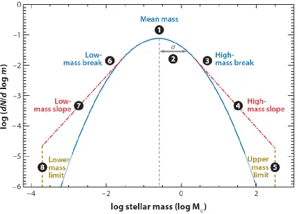
Surprisingly, the results of Salpeter (1955) seem to hold true for a number of other studies, over a large mass regime. The low-mass IMF has a shallower slope, before turning over (changing sign) at a characteristic mass before the lower mass cutoff (set by the limit of hydrogen burning), as displayed graphically in Figure 1. The sub-stellar and sub-solar IMFs are not addressed here, but see reviews by Bastian et al. (2010) and Kroupa (2005) for a more comprehensive review of those topics.
3 Equation 3 Kroupa IMF
where A is the normalization and the values of α are determined by the following relations:
Equation 4 Kroupa IMF exponents
The Scalo index (Scalo 1998) goes as α3=2.7+/-0.7 for 1<m/M, n=3, which is consistent within errors of
the Salpeter slope of α=2.35 and the Kroupa slope α2=2.3 (recall α=Γ+1, and note that in Equation 3 α is
taken to be a positive value with the negative built into the equation itself) and the results of Kroupa (2001).
4
[image:14.612.83.515.129.439.2]The primary concerns of this study are parameters 4 and 5 as labeled in Figure 1, the high mass slope and upper mass limit respectively.
Figure 1 Eight-Parameter IMF from Bastian et al. (2010)
5
Coeval populations of stars existing at the same spatial location provide for a far more straightforward measurement of the IMF. Such populations are found in stellar clusters and OB associations throughout the Milky Way and Magellanic Clouds. While OB associations have larger ages and age spreads, young massive stellar clusters have small age spreads (typically 1 Myr, though error on the age determination can be larger than 1 Myr). Single-age models are able to accurately represent the stellar populations in stellar clusters and most OB associations.
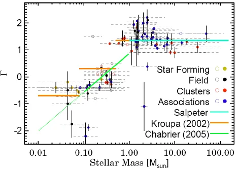
The slope of the IMF has been measured for several Galactic clusters and OB associations through direct counts (Kroupa 2002, references therein), but rarely for clusters massive enough to fully sample the high end of the mass spectrum (e.g. >10 M). Figure 2, taken from Bastian et al. (2010), illustrates this point. Though the data contained in this plot do not represent every IMF slope measurement available in the literature, the data are representative of the literature. Therefore the relative lack of measurements at the high mass regime remains evident. Comparing the slope of the IMF of several young, massive star clusters can directly test the claimed universality of the IMF for the sample examined. The larger the sample, the more statistical weight that can be placed on the results. Statistically significant deviations from the average in the measured slopes can be examined in the context of external environment, e.g. metallicity, Galactic location.
6
Figure 2 Selection of estimates of the IMF slope as a function of mass range, taken from Bastian et al. (2010)
A very careful definition of the term “initial mass function” is required to understand the goals and results of the investigation presented here. The IMF is defined as the inferred mass distribution of stars produced in a star formation event. Rarely is the initial distribution observed; instead the present-day population is observed. The IMF is then inferred from the present-day population.
To construct an IMF for a sample of clusters, evolutionary models are applied to infrared photometry. The photometry is calibrated via spectroscopic observations, which are used to determine luminosity class and distance. The evolved massive star population is used to constrain the age of individual clusters. The present-day mass of main sequence stars in each cluster is determined from magnitude-mass relations of rotating stellar evolutionary models (Maeder & Meynet 2003). From the present-day mass, the initial mass is inferred according to the same stellar evolutionary models.
7
estimates. This is especially evident from the large distance ranges in spectrophotometric distance calculations. Errors in the distance estimate subsequently produce errors in the absolute magnitude of objects in each cluster. The absolute magnitude and infrared colors are used to determine the present day mass of each star. The present day mass is directly related to the initial mass as per the mass-loss prescriptions of the stellar evolution models. The most massive stars have high mass-loss rates (Vink et al. 2000, 2001, 2011), which leads to rapid evolution away from the zero-age main sequence (ZAMS).
1.1.1.
Variations
Variations in measurements of the IMF slope can be attributed to any number of observational effects, including the effects of sample size, systematic error, presence of unresolved binaries, and field of view. Studies of the IMF in the Arches cluster show that the slope of the IMF changes with distance from the cluster center due to mass segregation. Restricted field of view limits the identification of observational evidence for mass segregation. Additional physical processes governing star formation, e.g. metallicity, Galactic location, can potentially affect the slope of the IMF.
To date, the strongest claim for a high end IMF slope significantly different from Salpeter arises from studies of the center of the Milky Way. Multiple authors (Bartko et al. 2010; Lue et al. 2013) find evidence for a flattened (larger number of massive stars than predicted by a Salpeter or Kroupa IMF slope) IMF is found in Galactic Center region. These results are consistent with X-ray studies of the Galactic Center. Nayakshin & Sunyaev 2005 find that scaling-up the X-ray population of the Orion Nebula Cluster is inconsistent with the X-ray flux of the Galactic Center.
1.1.2.
Stellar Evolution Models: Past and Present
The most important assumption of the stellar evolutionary models discussed here is the singularity of stars: no binary evolution (e.g. rejuvenation due to mass transfer) is incorporated into these grids of models. For a more thorough review of the effects of binarity on the evolution of massive stars, see Langer (2012) and references therein.
8
Broadened line profiles provide observational evidence for rotation in massive stars, which results in an enhancement of mass loss via stellar winds. The effects of rotation are thoroughly reviewed by Maeder & Meynet (2000), who go on to lead efforts to include rotation in stellar evolution models. More recently, Vink et al. (2011) calculates mass loss rates for very massive stars (up to 300 M), as an improvement upon previous work (Vink et al. 2000; Vink et al. 2001; Vink 2006). These authors emphasize the importance of rotation in stellar evolution models, calling for a “fundamental revision” in the incorporation of mass loss rates.
Calculations of rotating models have led to many important results. This includes the prediction of red supergiants at higher masses and luminosities than previously estimated from non-rotating models. Brott et al. (2011) show that stars as massive as 60 M can pass through the red supergiant phase at LMC metallcity. Eckstrom et al. (2012) demonstrate that the enhanced mass loss rates during the red supergiant phase can result in evolution back blueward for stars with initial masses in the range 15-20 M. These stars were previously thought to end their lifetimes as red supergiants before exploding as supernova. These recent studies emphasize the importance of including the effects of rotation in stellar evolution models.
Using the most recent set of Geneva stellar evolution models, in conjunction with the stellar atmosphere model results of CMFGEN (Hillier & Miller 1998), Groh et al. (2013) predict SNe from luminous blue variable (LBVs) in the initial mass range 20-25 M. Previously, stellar evolution models did not predict an LBV phase, potentially owing to the relatively short lifetime of this phase and the inability to reproduce the eruptions that define this phenomenological phase. Crockett et al. (2008) and Georgy et al. (2012) observe type IIb supernova having LBV progenitors, but no theoretical model had predicted that LBVs explode as supernovae until Groh et al. (2013).
Maeder & Meynet (2003) published a grid of rotating and non-rotating stellar evolution models from 8 to 120 M. The present study uses these models and the models of Schaerer et al. (1993), which have canonical mass-loss rates and cover the initial mass range of for 0.8 to 8.0 M. Brott et al. (2011) present a grid of evolutionary tracks from 5 to 60 M, incorporating rotation. Extrapolating these models up to nearly three times their mass (e.g. see R136 section of Results & Discussion) is less certain than extrapolating the Geneva models to only slightly higher masses.
1.1.3.
Method
9
mass cut-off. The importance of the upper mass limit is discussed below, along with techniques for determining such a limit.
The first step in constructing an IMF for the clusters in the sample presented here (discussed in depth in IMF Analysis) is to obtain deep, high resolution near-infrared (NIR) imaging. Optical observations suffer from the heavy extinctions towards these clusters, which are preferentially more distant and extinguished than clusters in previous IMF studies. Control fields are also observed to disentangle the cluster sequence from the fore- and background population. Near-IR photometry is used to select candidate cluster members for spectroscopic follow-up on the basis of color and magnitude. Once spectra have been obtained, spectral types are obtained via qualitative spectral typing. The results are used to determine some of the basic parameters of the cluster stars, e.g. temperature, luminosity class, cluster age. The IR colors and spectral types of the cluster stars are next used to estimate the extinction and spectrophotometric distance towards the cluster.
Figure 3 indicates how stellar atmosphere models can be applied to determine the fundamental properties of evolved massive stars, e.g. temperature and bolometric luminosity. Application of stellar atmosphere models to spectra of sufficient resolution and signal-to-noise (SNR) yields information such as metallicity, mass loss rate, current mass, and effective temperature. From these parameters the initial mass can be derived based on stellar evolution models and position on the Hertsprung-Russell (HR) diagram (see Figure 3). This information is key for determining the initial masses of post-MS stars, which are often located in degenerate parameter space of magnitude-mass relations drawn from evolution models alone.
10
Figure 3 IMF Flowchart: from image to IMF
In the context of this work, spectroscopy is used in a purely qualitative fashion: to calibrate the MS and identify post-MS stars in each cluster. Spectral typing is accurate to +/- 1 spectral type. A quantitative analysis of this spectra is ongoing as part of an analysis of the chemical cartography of the Galaxy (de la Fuente, PhD thesis work).
1.1.4.
Utilizing the IMF
11
Once this constant is determined, the total mass of the population can be found by integrating over the mass function,
Φ,
from ml to mu, where ml is the lower mass limit and mu is the upper mass limit (e.g 0.8to 150 M respectively for a Salpeter-type IMF). The slope of the mass function, Γ, is either imposed or calculated from the observations at hand. The derivation is as follows:
Equation 5 Mass derivation
1.2.
Upper Mass Cut Off
12 Equation 6
Schwarzschild & Harm (1959) determined that stars more massive than 60 M should be unstable to pulsations and the outer layers of the star are destroyed. Later work by Beech & Mitalas (1994) refined the calculation of Schwarzchild & Harm (1959), suggesting that pulsational instabilities could be damped, resulting in a larger theoretical limit. Improvements in the theoretical understanding of opacities (Rogers & Iglesia 1994) led to new calculations of upper mass limits that were also dependent on metallicity (Stothers 1992). Those calculations find that stars of 90-150 M remain stable against pulsations, while more massive stars are not.
Early statistical studies (e.g. Elmegreen 2000, Larson 2003) point out that random sampling of an IMF with no upper mass limit constraints predicts the existence of stars with M>1000 M. Super massive stars should be observed unless a previously unknown turn-down or truncation in the IMF exists beyond a few hundred M. The authors of these studies also emphasize that despite their predictions and the lack of observational evidence for 1000 M objects1, no upper mass limit had been observed.
Massey & Hunter (1998) find stars in R136 with masses of the order 140-155 M. Massey (2003) asserts that this is a statistical limit rather than a physical limit to the upper mass of stars. Figer (2005) finds stars in the Arches cluster with masses ranging up to 130-150 M, producing a cliff-like feature in the IMF (reproduced in Figure 4). Without an upper mass limit truncating the IMF, Figer (2005) predicts an additional 18 to 33 stars beyond the 130-150 M bin with masses up to 500 M. Extending his analysis of the Arches cluster to R136, Figer (2005) predicts at least 20 stars in R136 with masses greater than 150 M, ranging up to 750 M. Similarly, Weidner & Kroupa (2004) find that 40 stars with M > 150 M are “missing” from R136, assuming a total cluster mass of 5(104
) M. While the VLT-FLAMES survey has identified massive runaway stars originating from R136, far fewer than 20 of these objects have been identified.
Oey & Clarke (2005) present a statistical argument for an upper mass limit of 150 M based on a compilation of studies of massive stars and massive clusters in the literature. These authors assume a Salpeter-like IMF. Additionally, Koen (2006) examine the high mass regime of the IMF in R136 using
13
two statistical methods, finding an upper mass limit of 140 to 160 M. These results are consistent with the upper mass limit of 150 M found by Figer (2005).
Figure 4 IMF of Arches cluster, reproduced from Figer (2005)
14
1.3.
Young Massive Clusters and Candidate Clusters
Young, massive clusters (YMCs) are excellent probes of the high end of the IMF. YMCs represent coeval stellar populations. Massive star formation in stellar clusters occurs within a timescale that is less than the lifetime of the most massive stars, on the order of 1-2 Myr. Infrared-selected YMCs are preferentially more distant than their optical counterparts, probing a larger parameter space than previously available. Over the past 15 years, pioneering work in infrared detectors has ushered in a new era of large scale IR imaging surveys. The 2 Micron All Sky Survey (2MASS, Skrutskie et al. 2006) and Galactic Legacy Infrared Mid-Plane Survey Extraordinaire (GLIMPSE, Benjamin et al. 2003) have probed the Galactic Plane as never before. 2MASS began imaging the sky from the ground in 1997, completing the survey in 2001. This all-sky survey covered the entire sky at 1.25, 1.65, and 2.17 microns. The final GLIMPSE survey spans 300 degrees of the Galaxy with IRAC onboard the Spitzer Space Telescope. GLIMPSE provided imaging at 3.6, 4.5, 5.8, and 8.0 microns. Several groups searched through these two surveys for previously undiscovered stellar clusters (Dutra & Bica 2001, Bica et al. 2003, Dutra et al. 2003, Mercer et al. 2005, Froebrich et al. 2007), yielding thousands of candidate clusters.
Froebrich et al. (2007) use star density maps constructed from 2MASS data to search for stellar overdensities in the galactic plane. Other authors, notably Duta & Bica (2001), Bica et al. (2003), and Dutra et al. (2003), perform searches by eye in the direction of optical and radio nebulae. The group led by Froebrich estimates a contamination rate of up to 50% for their candidate cluster catalog, while the latter group make no estimates of contamination. Borissova et al. (2005) follow up 21 clusters from the catalogs of Bica et al. (2003) and Dutra et al. (2003), finding 7 genuine clusters. The remaining candidate clusters are found to be chance stellar overdensities, usually a result of patchy extinction. Mercer et al. (2005) used an automated search algorithm combined with visual inspection of the GLIMPSE mid-IR survey data to find 92 new cluster candidates. This catalog has been particularly successful: resulting in the identification of two new globular clusters in the plane of the galaxy (Mercer 3, Strader & Kobulnicky 2008; Mercer 5, Longmore et al. 2011) and several young, massive clusters (Mercer 30, Kurtev et al. 2007; Mercer 20, Messineo et al. 2009; Mercer 23, Hanson et al. 2010).
15
Magellanic Cloud (LMC) serves as a check with previous measurements and ensures that the largest mass range possible will be probed by this study. Observations of R136 are included in this work.
The sample presented here is drawn primarily from Hubble Space Telescope (HST) Near-Infrared Camera 3 (NIC3) imaging observations (P.I. Davies). The resolution of NIC3 is a large improvement on earlier imaging capabilities, such as those used in the studies of Massey et al. (1995a,b) for previous IMF determinations. Additionally, Very Large Telescope (VLT) NIR spectroscopy is available for the majority of the HST observations (VLT/ISAAC, P.I. de la Fuente), as well as Chandra X-ray Observatory (CXO) imaging for a smaller subset of the sample. Spectroscopy is used for spectral typing and CXO imaging is used to identify potential colliding wind binary systems.
A direct re-measurement of the IMF of the clusters examined by Massey et al. (1995a,b) results would be of great interest to the IMF community. However, an exact replication of the imaging and spectroscopy would be required to allow for comparisons to embedded Galactic clusters. Improved imaging, with higher resolution and sufficient photometric depth, is not available for the majority of the Massey et al. (1995a, b), Oey & Massey (1995), or Oey (1996) samples. The mass ranges probed by the previously mentioned samples are too low for a study of the high end IMF. Measuring the IMF slope above 10 M requires the discovery of additional young, massive (>104 M) clusters. Such a population is predicted to exist (Hanson et al. 2008, Ivanov et al. 2010), but remains largely undiscovered.
This study examines newly discovered candidate stellar clusters. The goal is to provide a similar investigation of the intermediate to high mass range of the IMF as presented in Massey (1998). To achieve this goal, the slope of the IMF is computed for young, massive clusters drawn from the same set of observations. For example, HST NIR imaging provides all the photometric data presented in this work, with the exception of R136. Spectroscopy of southern objects is obtained with VLT/ISAAC and nothern objects with IRTF/SpeX.
17
2.
Observations
2.1.
Sample of Cluster Candidates
The initial sample of candidate young, massive clusters was drawn from an archive of hundreds of candidates built by combining the catalogs of Dutra et al. (2001), Bica et al. (2003), Dutra et al. (2003), and Mercer et al. (2005). For each catalog object, a webpage was created containing a 2MASS 3-color image, a GLIMPSE 3-color image where available, and 2MASS color-magnitude diagrams (H-K vs. K and J-K vs. K) containing all point sources in the 2MASS image. As the project evolved, additional information was added to each candidate webpage where possible, e.g. HST images, HST color-magnitude diagrams, CXO observations, spectroscopic observations, and radio observations.
Before the completion of GLIMPSE-II, a Spitzer/IRAC proposal (Program 30734, PI Figer) was submitted for 76 candidate clusters which showed promise but were not covered by GLIMPSE-I. The observations were specifically designed to mimic the GLIMPSE observing strategy, in order to make the targeted fields directly comparable to GLIMPSE fields. The objects observed in this program are listed below in Table 1. There are no Mercer et al. (2005) objects in the Spizter proposal; the Mercer object list was created by examining 2MASS and GLIMPSE, both by eye and with an automated algorithm.
The “best” candidate young, massive clusters were then drawn from the Spitzer observations of Bica/Dutra clusters and the Mercer catalog. These clusters were chosen based on several criteria: stellar over density discernible by eye, signposts of youth (including the presence of natal material, in many cases a bubble or partial bubble in the surrounding ISM), IR color-magnitude diagram indicating a main sequence. HST proposal ID 11545 (PI Davies) was designed to observe 29 candidate clusters using filters F160W, F187N, F190N, and F222M with NICMOS/NIC3.
Follow-up spectroscopy was obtained to determine parameters, e.g. spectral type, of stars on the main sequence, identify evolved cluster stars, and identify fore- and background non-cluster members for each set of observations. Southern clusters in the sample were observed using VLT/ISAAC (PI la Fuente), and northern clusters were observed using IRTF/SpeX (PI Trombley). Spectra in the work presented here is plotted as flux per unit wavelength.
2.2.
Spizter/IRAC Imaging: Reduction and Photometry
Table 1 Spizter/IRAC Targets18
19
DBSB2003T3+26 8 46 34 -43 54 28 DBSB2003T3+28 8 56 28 -43 05 53 DBSB2003T3+33 9 01 54 -47 43 53 DBSB2003T3+35 9 15 11 -47 28 32 DBSB2003T3+36 9 16 44 -47 56 28 DBSB2003T3+37 9 22 12 -48 05 02 DBSB2003T3+38 9 24 25 -51 59 28 DBSB2003T3+4 7 32 10 -16 58 15 DBSB2003T3+44 10 15 51 -57 23 38 DBSB2003T3+45 10 19 11 -58 02 21 DBSB2003T3+48 10 31 29 -58 02 01 DBSB2003T3+54 10 43 57 -59 32 56 DBSB2003T3+59 11 12 18 -58 46 18 DBSB2003T3+60 11 05 37 -62 28 57 DBSB2003T3+67 11 30 07 -62 03 32 DBSB2003T3+7 7 35 34 -18 45 34 DBSB2003T3+74 12 10 00 -62 49 52 DBSB2003T3+75 12 09 02 -63 15 54 DBSB2003T3+76 12 22 30 -63 17 35 DBSB2003T3+8 7 35 39 -18 48 50 DBSB2003T3+87 13 32 47 -60 26 54 DBSB2003T4+125 9 59 32 -57 04 05 DBSB2003T4+126 10 06 40 -57 12 33
Spizter Program 30734 (PI Figer) was designed to mimic the GLIMPSE observing cadence, taking images in all four IRAC bands or channels, 3.6, 4.5, 5.8, and 8.0 microns, and providing a resolution of 0.6 arcseconds. Each set of IRAC basic calibrated data (bcd) was retrieved via the Leopard tool from the Spizter Science Center (SSC), then mosaicked using Mopex, also operated and maintained by SSC. Channels 1 and 2, correspondig to 3.6 and 4.5 microns respectively consisted of 20 overlapping fields, or tiles, while channels 3 and 4, 5.8 ad 8.0 micros respectively, were made up of 10 fields. In some cases, e.g. [BDS2003] 52 in Figure 5, problems in one or more header files made it necessary to mosaic the channel 4 observations by hand.
20
micron image. The adverse effects can be seen in Figure 5, in which the left hand panel clearly shows a misplaced tile.
Several bright non-saturated point sources were chosen as references points for mosaics made by hand. The centroid of each source in each overlapping frame was determined using GCNTRD.PRO, from the IDL Astronomy User’s Library. One frame was chosen to be the reference frame, or 0th
position, and the remaining frames were offset as computed from the positions of the bright sources. Three bright non-saturated point sources with corresponding non-non-saturated point sources in channel 1 were selected for finding theastrometry solution, applied by using STARAST.PRO from the IDL Astronomy User’s Library.
Figure 5 Left: Pipeline mosaicked image of [BDS2003] 52 Right: Hand mosaciked image of [BDS2003] 52
21
SSC IRAC data handbook. Aperture photometry using APER.PRO was done separately on each frame, and the results cross-correlated to build a final catalog of photometry for each cluster candidate. Catalog criteria required valid photometric points in two or more channels to avoid inclusion of spurious sources. The sources in the final catalog were cross-correlated with the 2MASS Point Source catalog, and associations were made when positions of IRAC sources were within 4 arcseconds of a 2MASS source. For (rare) cases of double detections, association preference was given to the closest object.
Aperture photometry was found to be yield better results than point source function (PSF) photometry for the Spitzer/IRAC imaging. This is largely due to the diffuse emission present in nearly every band in every wavelength. The presence of bright, diffuse emission made locating isolated, bright stars for PSF characterization difficult. PSF fitting was further complicated by the diffuse emission, resulting in in poor PSF photometry.
2.3.
HST/NIC3 Imaging: Reduction and Photometry
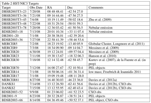
Hubble Space Telescope (HST) Near Infrared Camera 3 (NIC3) observations were taken in the summer of 2008 as part of ProgID 11545 (PI Davies). The observations were taken in a 6-position spiral dither Table 2 HST/NIC3 Targets
Target Obs Date RA Dec Comments DBSB2003T3+23 7/20/08 08 48 48.41 -42 54 27.0
DBSB2003T3+36 7/21/08 09 16 44.46 -47 56 27.5
DBSB2003T3+45 7/6/08 10 19 11.49 -58 02 18.6 Zhu et al. (2009) DBSB2003T3+48 7/22/08 10 31 29.54 -58 01 59.3
DBSB2003T3+78 7/20/08 12 36 03.42 -61 50 56.5 Nebular emission BDSB2003+18 7/13/08 20 01 10.34 +33 11 07.4 Nebular emission DB2001+20 7/1/08 20 38 38.01 +42 39 20.6
BDSB2003+36 7/27/08 22 58 41.39 +58 46 53.6
MERCER5 7/2/08 18 23 19.92 -13 40 05.9 Globular Cluster, Longmore et al. (2011) MERCER9 7/3/08 18 34 09.90 -09 14 04.7 Messineo et al. (2009)
MERCER20 6/30/08 19 12 24.01 +09 57 04.4 Messineo et al. (2009) MERCER23 7/11/08 19 30 13.67 +18 32 06.3 Hanson et al. (2010)
MERCER30 7/18/08 12 14 32.48 -62 58 45.7 Kurtev et al. (2007), de la Fuente et al. (in prep)
MERCER70 7/12/08 16 00 27.67 -52 10 50.4 PEL objects
MERCER14 7/1/08 18 58 06.16 +01 36 31.4 low mass; Froebrich & Ioannidis 2011 MERCER17 7/1/08 19 09 19.48 +08 11 28.0
MERCER81 8/27/08 16 40 30.03 -46 23 36.0 Davies et al. (2012a)
DANKS1 7/14/08 13 12 26.50 -62 41 56.6 Davies et al. (2012b), CXO obs DANKS2 7/15/08 13 12 55.95 -62 40 43.4 Davies et al. (2012b), CXO obs BDSB2003+52 9/9/08 01 23 06.02 +61 52 23.5 CXO obs
DB2001+9 8/23/08 20 32 28.87 +38 51 24.1 PEL objects
[image:31.612.63.553.320.656.2]22
pattern with an offset of 5.07 arseconds and carefully reduced in order to counteract the known under-sampled PSF of the NIC3 detector. Each candidate cluster was observed in four filters: F160W, F187N, F190N, and F222M, while a near-by control field of identical size was observed only in wide band filters, F160W and F222M.
The raw data for each visit was retrieved using the Barbara A. Mikulski Archive for Space Telescopes (MAST) HST search form. Each raw image was resampled onto a finer grid, then combined using IDL routines NICMOSAIC.PRO and NICSTIKUM.PRO. The overlap parameters were determined by NICMOSAIC.PRO and the final image was combined by NICSTIKUM.PRO to produce a science-quality frame.
23
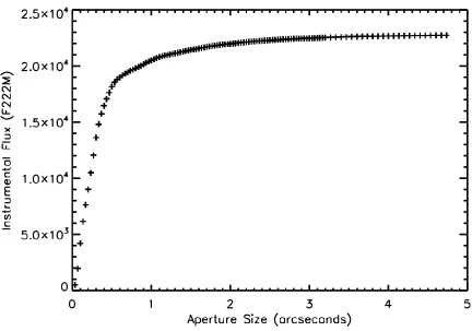
Figure 6 Aperture size vs. encircled flux
The aperture radius was chosen to be 6 pixels, with an annulus of 20-30 pixels for background characterization, corresponding to an angular size of 0.4 arcseconds and 1.3 to 2.0 arcseconds. Similar analysis was done for two clusters using PSF photometry from StarFinder, with minimal discrepancies (Davies et al. 2012b). Sources due to contamination from diffraction spikes and Airy rings of very bright objects were visually identified and removed by hand in order to obtain the best photometric results possible.
24
stars than for bright stars, potentially flattening the constructed IMF by overestimating the mass of the less massive stars.
Photometry was then used to construct color-magnitude diagrams for each cluster/field combination, where the control field is intended to be used as an indicator of the contaminating fore- and background population. Narrow-band photometry was utilized to identify emission line objects. Both the color-magnitude diagrams and emission line objects are discussed in further detail in the Data Analysis chapter.
2.4.
VLT/ISAAC Spectroscopy: Observations and Reduction
Table 3 VLT/ISAAC Targets
Target RA Dec Band(s) Mercer 81 16 40 24 -46 23 36 H, K1, K2 Mercer 20 19 12 25 +09 57 42 H, K1, K2 Mercer 70 16 00 27 -52 10 48 H, K1, K2 Mercer 23 19 30 13.1 +18 32 09 H, K1, K2 Danks 1 13 12 27 -62 42 06 H, K1, K2 Danks 2 13 12 55 -62 40 56 H, K1, K2 Mercer 30 12 14 32.0 -62 58 49 H, K1, K2
Southern cluster candidates, listed in Table 3, were observed spectroscopically in the near-IR using ISAAC at the VLT. This effort was led by Diego de la Fuente, from proposal to reduction. Examples of his work can be found in Davies et al. (2012a), including the reduction procedure. In a few words, the spectral observations were reduced via customized spectroscopic reduction IDL code written by Ben Davies, and adapted by Diego de la Fuente for use with the VLT/ISAAC observations. For each pointing, nod pairs were subtracted to remove sky features and the result flat-fielded. The resulting 2D frames were rectified and wavelength calibrated using arc frames, after which each spectrum was extracted then divided by a telluric standard star (see section 2.2 and Fig 5 of Davies et al. 2012a for the specific example of Mercer 81) to produce the science spectrum.
25
2.5.
IRTF/SpeX Spectroscsopy: Observations and Reduction
Table 4 IRTF/SpeX TargetsObject Date of Obs RA Declination Mercer 17 7 Sept 2012 19 09 19 +08 11 42 [DB2001] Cl 9 7 Sept 2012 20 32 27.8 +38 51 26 [DB2001] Cl 20 7 Sept 2012
18 Sept 2012
20 38 37 +42 39 24 [BDS2003] 52 7 Sept 2012
18 Sept 2012
01 23 06 +61 51 24 [BDS2003] 66 18 Sept 2012 04 36 50 +50 52 48 HD28794 18 Sept 2012 04 34 45.942 +50 07
28.23 HD196503 7 Sept 2012
18 Sept 2012
20 36 27.869 +41 02 03 HD195377 7 Sept 2012 20 29 28.25 +38 57
05.58 HD8013 7 Sept 2012
18 Sept 2012
01 20 52.149 +60 56 56.10 HD178162 7 Sept 2012 19 07 11.225 +08 20
56.44 HD195377 7 Sept 2012 20 29 28.259 +38 57
05.58
27
Figure 7 Finding charts for IRTF/SpeX runs. In all images, North is up and East is left. From left to right, top to bottom: Mercer17, [BDS2003] 52, [DB2001] Cl 9, [DB2001] Cl 20, [BDS2003] 66, and
[BDS2003] 36.
Reduction of observations taken on 8 September 2012, 18 September 2012, and 20 January were completed using the Spextool 3.4 package (Cushings et al. 2004). Finding charts for each cluster can be found in Figure 7. Spectra were taken in an ABBA nodding pattern throughout all nights. Integration times were based on the sensitivity parameters given on the IRTF webpage for the K band, including use of the SpeX integration time/SNR calculator. Standard stars of A0V spectral type at similar airmass to target stars were observed multiple times. Master arcs and flats were made from calibration files (using the sxd0.3cal macro) taken throughout the night. This process also provides a wavelength solution used to calibrate the raw spectra. Frames were nod-subtracted then flat fielded, and orders with high enough signal to noise extracted and wavelength calibrated. Extracted spectra were next divided by a scaled telluric standard star of similar airmass, resulting in flux-calibrated spectra.
On the night of 18 September 2012, extracted spectra were examined during the run “on the fly” in order to decide if other objects in the field of view should be observed. In the case of [BDS2003] 66, two fainter stars were observed in order to test that a potential main sequence was not actually comprised of foreground giants (both objects were easily identified as hot stars).
28
[image:38.612.137.467.91.320.2]2.6.
Keck II/NIRC2 Imaging and Slitless Spectroscopy: Observations and Reduction
Table 5 Keck II/NIRC2 TargetsTarget Filter Mode Int Time (s) Date
Mercer 5 J imaging 3 23 August 2008 H imaging 3 23 August 2008 Ks imaging 1.2 23 August 2008 CO imaging 20 23 August 2008 Kcon imaging 20 23 August 2008 Control Field H imaging 2 23 August 2008 Ks imaging 1.2 23 August 2008 Mercer 5 Br
γ
grism 40 23 August 2008 CO grism 40 23 August 2008 BD-14 5029 Brγ
grism 3 23 August 2008 CO grism 3 23 August 2008 Arches Brγ
grism 240 12 July 2011CO grism 240 12 July 2011 q3 Br
γ
grism 30 12 July 2011 CO grism 30 12 July 2011Two clusters were observed in the near-IR using the Near Infrared Camera 2 (NIRC2) at Keck II: Mercer 5 on 23 August 2008 and the Arches on 12 July 2011.
2.6.1.
Laser Guide Star Adaptive Optics Imaging
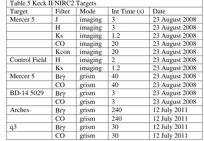
The high density of Mercer 5 was immediately apparent from visual inspection of the HST/NIC3 imaging, suggesting that observations at higher spatial resolution were necessary. To this aim, the cluster was observed using Keck II/NIRC2 in the J, H, and K bands utilizing the laser guide star adaptive optics (LGASO) system. The area corresponding to the HST control field for Mercer 5 was also observed in the H and K filters. Twenty overlapping images were taken, resulting in a total exposure time of 60 seconds in J and H and 24 seconds in K. The observations are nearly diffraction limited, with point sources having a FWHM of ~60 mas in the Ks band.
29
Figure 8 Ks band NIRC2 LGSAO image
30
2MASS point source catalog. Resulting color-magnitude diagrams include those in Figure 16, which are discussed in the Mercer 5 section of Chapter 3.
Astrometric calibration of the NIRC2 frames was calculated using positions of point sources in the HST observations by applying the IDL routine STARAST.PRO; three stars common to both the HST and NIRC2 observations were used to compute a geometric transformation for both the cluster and control field separately.
31
32
2.6.2.
Slitless Spectroscopy
Grism spectroscopy was taken for both Mercer 5 and the Arches stellar clusters, using narrowband filters centered on Bracket Gamma (Brγ
,
2.166 microns) and the first CO bandhead (2.2891 micros). The use of narrowband filters provides a spectral “snippet” of every star in the field of view of the detector down to some limiting magnitude. The x,y positions of the center of the spectral snippet corresponds to the x,y positions of the target stars in the non-grism imaging field of view. Brγ
and CO were chosen because each provides a quick determinate of rough spectral type: Brγ
emission or absorption is observed in hot stars while CO features are only present in cool stars, e.g. red giants or red supergiants.2.6.2.1.
Mercer 5
33
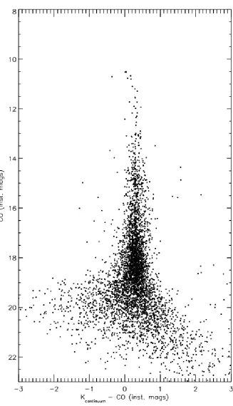
Figure 10 Raw spectra of two objects blend together, in black and on the left, resulting in no information about either object. Example of single spectrum is shown in blue, to the right of the blended spectra.
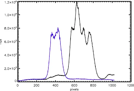
Figure 11 Left: CO narrowband filter profile; Mercer 5 target star shown in black (with deep absorption feature), standard star shown in red. Both spectra have been normalized to 1. Right: Brγ narrowband filter
34
The raw images were dark subtracted and field fielded in the usual way. Inspection of the Br
γ
flat fields revealed them to be saturated, but the CO calibration files were within acceptable limits. A standard star (BD-14 5029 of spectral type B1.5b) was observed in the same manner as the cluster and spectra extracted in an identical manner. Again, reduction and extraction could only be done for the CO narrowband observations. An example frame containing CO narrowband slitless spectroscopy of Mercer is presented in Figure 12.35
Source detection was performed on each frame by stepping across in the x-direction (in steps of 25 pixels) and identifying peaks in the y-direction above a certain threshold. Using this method, columns containing a sharp peak were flagged as containing at least one object, often multiple objects given the high density of the target, then the row containing each peak was searched for spectra. Visual inspection indicated that each spectrum spans roughly 100 pixels (e.g. see Figure 11). A background value was calculated for each flagged row, then pixels above that background were counted. Objects that were cut off by the edge of the frame were discarded as having too few pixels above the background. Some rows contained multiple spectra, all of which were flagged, leading to double detections. Double detections were common and removed via an automated process after source detection. Some sources were missed entirely and added by hand after the detection process was complete.
Spectral extraction began once the detection algorithm reached the end of the frame and double detections were removed from the list of flagged objects. The profile of the CO filter has a shape such that two distinct peaks are present in each spectrum, one higher than the other (as seen in the left panel of Figure 11). As all of the stars in Mercer 5 are expected to be cool, only absorption lines should be present in the wavelength regime covered by the CO filter. An example of this is shown in Figure 11, with the standard star in red displayed as a proxy for the filter profile. This filter profile allows for use of the highest peak as a common defining point in each spectrum. Raw spectra were extracted using a width of 150 pixels and a height of 5 pixels. The five pixel rows were collapsed into a 1D spectrum which was written to a fits file.
Each target spectrum was divided by the normalized standard to remove the filter profile shape and sky contribution. Wavelength calibration was performed using half-power points, in theory corresponding to the cut-on and cut-off wavelengths of the filter. The half-power points were taken from the instrument specifications listed in the manual. The spectral resolution was then calculated by dividing the central wavelength of the CO filter, 2.2891 microns, by the FWHM of the CO image, multiplied by the linear dispersion. This method yielded a resolution of R~1420. Spectra were extracted from all 7 frames then cross-correlated and summed to produce a final spectrum of each star. An example of the raw extraction is shown in Figure 11, the cluster star in black and the standard star in red. Notice the characteristic absorption feature in the center of the filter profile for the cluster star. In the best case scenario, an object was covered in all 7 pointings and the final spectrum built from 7 raw spectra.
36
degraded to the resolution of the target stars, then shifted in wavelength to match the deepest point in the CO bandhead. The results of this comparison are discussed below.
2.6.2.2.
Arches
For the Arches observations, three position angles were chosen: 0, 30, and 60 degrees. This was done to allow for characterization of objects which were blended in a single position angle, as shown in Figure 10 above. The Quintuplet star q3 was observed as a telluric standard, chosen on the basis of a lack of spectral features (both emission and absorption) in the K-band. Two observations of q3 were taken using the Br
γ
filter, with exposure times 120 sec and 30 sec. However, the standard star was found to be saturated in all Brγ
exposures and only partially contained in the CO exposure. The saturated spectrum is shown in Figure 13. Luckily, [CEC96] F was present in the field of view of the Arches target observations, and could be used as a standard star in both Brγ
and CO. This object is classified as a foreground star based on its photometric properties (i.e. its color appears bluer than the rest of the Arches cluster). Only one of the three target frames contained a suitable spectrum of [CEC96] F; the star was absent or partially cut off in the other frames.37
Calibration files for the Arches observations were not taken the same night as the science observations. Flats from the archive were found to be saturated, and NIRC2 was not used again for several weeks. It was necessary to wait some time for the appropriate calibration files. A modified version of the Mercer 5 IDL code was used to reduce and extract spectra in the same manner. Extraction of spectra in the Arches cluster was complicated by the nature of the target objects: Br
γ
is found in emission in very hot massive stars, often in excess of the two peaks of the filter profile. This made it difficult to assign the same common defining point in all objects as done for Mercer 5. For some extreme cases, the Brγ
emission filled the majority of wavelength space. Spectra of WNL stars heavily dominate the Brγ
emission in the Arches slitless spectroscopy frames, often leading to contamination of both near-by and not as near-by objects.2.7.
Chandra/ACIS: Reduction
Table 6 CXO/ACIS TargetsTarget RA Dec Int Time (ks) ID Comment [BDS2003] 52 01 23 06 +61 51 24 10 6575
[BDS2003] 66 04 36 50 +50 52 48 10 7478
G305 13 12 27 -62 42 06 125 8922 Danks 2 falls on chip gap [DB2001] Cl 20 20 38 37 +42 39 24 30 8893 Fall on chip gap
Mercer 81 16 40 24 -46 23 36 40 11008
The CXO deliverable “images” do not need to be reduced. Each set of raw data includes a file named “acisfID#N001_evt2.fits” which contains the level 2 events (level 2 events have been irreversibly filtered for good time intervals, cosmic ray rejection, and pixel position transformation to astromertric coordinates). Generally, observations are binned to a certain extent and visualized in different manners. Point source extraction varies from observation to observation, and is discussed in individual cluster sections along with the point source analysis and cross-correlation of sources.
2.8.
VLT/MAD Imaging: Photometry in the core of R136
38
39
Figure 14 MAD Ks-band image of R136
2.9.
Completeness Tests
40
2.9.1.
VLT/MAD Completeness Procedure
The core of R136 as observed by VLT/MAD is only complete to roughly 30 M. Completeness was investigated via the artificial star method: artificial stars over a wide range of magnitude were added to each frame, for both the cluster center and the two control fields. Photometry was then redone in an identical manner to the science frames in order to characterize the recovery of the artificial stars. This test was repeated 100 times for both H and Ks bands in order to obtain robust completeness results. Identical procedures were run for each field, the core of R136, control field A, and control field B. The results of the completeness test for the R136 cluster core (black plus symbols) and both control fields (red asterisks, blue diamonds) is shown in Figure 15. This figure demonstrates how crowding in the cluster core causes the completeness to drop at brighter magnitudes than in the control fields (beginning around KS~17 mag).
41
Figure 15 Completeness as a function of magnitude in the core of R136 and both control fields as observed by VLT/MAD.
2.9.2.
HST/NIC3 Completeness Procedure
The artificial star method was also used to investigate the photometric completeness of HST/NIC3 observations, though the procedure varied slightly from the VLT/MAD imaging. For each of 100 iterations, 47 artificial stars varying in magnitude from 8.5 to 20 mag were added to each field. The x and y position of each artificial star was randomly assigned in a repeatable way. The PSF of NIC3 has been well modeled by John Krist and Richard Hook, who publish and maintain the Tiny Tim software. Tiny Tim is designed to compute a position-dependent PSF for each of the HST cameras. A parameter file, which can be generated in batch mode, is used to determine the parameters of the resulting PSF(s). These parameters include camera, detector, x and y position, and magnitude, to name a few. For each artificial star, a parameter file was written and Tiny Tim called from IDL to create the appropriate PSF. Each resulting PSF was added to the observed image, and photometry redone in an identical manner to the science photometry.
42
43
3.
Data Analysis
A selection of the candidate clusters listed in Table 2 are discussed in detail in this chapter. The nature of each candidate – genuine cluster or spurious detection – is examined and, in the case of real clusters, the basic parameters such as age, distance, stellar content, reddening, and total cluster mass, are derived. Given the robust selection criteria for identifying young, massive clusters for follow-up, it is of little surprise that most candidates are true clusters. For each cluster, the age, total mass, and stellar content are used to determine whether a measurement of the slope of the initial mass function would be a useful contribution to the overall project goals. In the case of older (>~6 Myr) clusters, the majority of massive stars have already left the main sequence. In these clusters, the high mass limit to the IMF slope measurement suffers. For lower mass (~103 M) clusters, the stellar content at the high mass end is prone to small number fluctuations, resulting in high errors on any IMF slope measurements.
3.1.
Mercer 5
Inspection of the HST images of Mercer 5 reveal a very dense cluster; the HST CMD reveals a red clump at mF222M ~ 13 mag, suggesting an advanced cluster age (>100 Myr). Though this instantly removes Mercer 5 from the IMF slope project, the cluster on its own is interesting enough to warrant further study. To this aim, higher resolution imaging was required to better investigate the stellar population. Laser guide star adaptive optics (LGSAO) imaging was obtained in the J, H, Ks, Kcon, CO, and Br
γ
bands using NIRC2 at Keck II. Slitless spectroscopy using the CO and Brγ
narrowband filterss was also obtained the same night. Analysis of the LGSAO imaging results is discussed below. In short, Mercer 5 is found to be a newly discovered globular cluster in the Galactic Plane (see also Longmore et al. 2011).3.1.1.
NIR Imaging
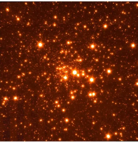
44
Figure 16 Left: NIRC2 CMD for Mercer 5 Right: NIRC2 CMD for control field. The control field is not overplotted on the cluster field of view to avoid confusion due to the dense nature of both fields.
3.1.2.
Slitless Spectroscopy
45
Figure 17 Left: Selected spectra of photometrically selected red clump stars. Right: Selected spectra of bright stars.
46
[image:56.612.114.488.87.348.2]Figure 18 EW vs. spectral type for cool giants, supergiants. Overplotted are the EW and spectral type of the average spectra of red giant branch and red clump stars in Mercer 5.
47
3.1.3.
Metallicity
The two populations of globular clusters belonging to the Milky Way appear to follow a trend. The halo population consists of metal-poor globulars, while the bulge population is made up of higher metallicity globulars. In order to determine if Mercer 5 is merely passing through the Galactic plane or belongs to the bulge population, measurement of radial velocity, proper motion, and/or metallicity are required. Without the availability of sufficiently high resolution spectroscopy to determine radial velocities or multi-epoch monitoring to determine proper motion, only metallicity can provide a hint to the origin of Mercer 5. It has been shown for other globular and open clusters in the Galaxy that the IR slope of the red giant branch (RGB) in K vs. J-K space varies according to metallicity (Kuchinski et al. 1995; Ferraro et al. 2000; Valenti et al. 2004). Valenti et al. (2004) find the relation [Fe/H]=-22.21x(slope RGB)-2.80, using a linear least squares fit to the decontaminated red giant branch of 10 Galactic Globular clusters. These authors fit the RGB from 0.5 mag to 5.0 mag fainter than the brightest stars. The results of that work are re-examined in Valenti et al. (2007), in which the authors find good agreement between their metallicity determinations and metallicity values published in the literature for 24 bulge globular clusters.
The metal-rich old open cluster NGC 6791, examined in the infrared by Carney et al. (2005), does not follow the RGB slope-metallicity relationships published by Valenti et al. (2004, 2007). These authors determine their own RGB slope-metallicity fit (Eqn 5 in Carney et al. 2005) but find poor agreement between their predictions and spectroscopic metallicity measurements of NGC 6791. As a result, these authors suggest that the RGB slope is only linear in a restricted metallicity range, [Fe/H]<=-0.3, or is not linear in K vs. J-K space.
In an attempt to roughly determine the metallicity of Mercer 5, a 2nd order polynomial was fit to the red giant branch at increasing inclusion radii up to the full angular extent of the NIRC2 imaging. These fits included stars from KS~14 mag to KS~9 mag between 3.0 < J-KS < 4.0. The relationship established in
48
3.1.4.
Mass, Age, and Distance
The mass of Mercer 5 was investigated using multiple methods. Integrating the stellar density function over the radial profile of the cluster is one way to estimate the total mass of the cluster, but this method has some drawbacks. The high density of the cluster gives makes this measurement highly incomplete, especially near the cluster center.
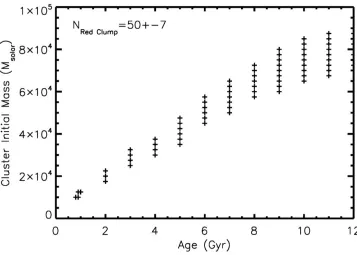
Another method of computing the total mass of the cluster is by counting the number of red clump stars (~50) and comparing to Geneva stellar population model predictions, as shown in Figure 20. These models are age dependent, yielding the same result for different combinations of age and total cluster masses. This method yields a mass of 2(104) M if the cluster is older than ~1 Gyr, increasing with increasing age. Similarly, for a younger age (~100 Myr) the total mass estimate is lower, below 104 M. Thus, it is necessary to determine the age of the cluster in order to place a stronger constraint on the cluster mass.
One method to determine the age of the cluster is to use the Ks-band luminosity function; the ratio of the number of stars in the red clump compared to the number in the nearby gap is a strong function of age. In the luminosity function, Figure 21, it can be seen that this ratio is ~5, corresponding to an age of 1 Gyr or older. Note that for younger clusters, this ratio will be much larger (e.g. ~50 for an age of ~100 Myr). The distance between the red clump and the MS turn-off can also be used as an age estimator, though this was complicated by the effects of differential reddening and the smearing out of the red clump in the KS band
49
[image:59.612.120.477.92.347.2]Figure 20 Mtotal vs. expected Nred clump stars
Figure 21 Thick black lines: KS-band de-reddened luminosity function of Mercer 5; the red clump can be
seen as the excess at KS~13 mag. The left hand panel shows age models (thin black lines) for LMC
metallicity, while the right hand panel shows ages models (thin black lines) for solar metallicity. For both metallicities, a model age of 10 Gyr or higher fits the data best. The sharp drop at KS=18 is due to
incompleteness.
50 Equation 7
where
Equation 8
given (H-Ks)0 = 0.3 for red clump stars and AH/AKs = 1.44 (Rieke et al 1989). For an old (>1Gyr) cluster,
this gives a distance modulus (mKs,0 – MKs,0)=12.8-1.6=14.4 or roughly 8 kpc.
Another crude distance estimator uses the brightest stars in a globular cluster as a standard candle (Frogel et al. 1981). The absolute magnitudes of these stars are shown to be a function of metallicity; without a priori knowledge of the metallicity and cluster membership of Mercer 5, it is only possible to relate the apparent magnitude of the brightest “cluster” star to the average metallicity value. For the case of Mercer 5, the brightest object in the field of view was assumed to be a cluster member. This is a valid assumption as the brightest stars are centrally concentrated, consistent with globular cluster dynamical evolution, and the brightest star is not significantly displaced from the cluster center. For the average over 10 clusters of varying metallicity in Table 6 of Ferraro et al. (2000), it is shown that MK,TIP,0=-6.29+/-0.45 (where the
error is the standard deviation of the sample). Using this average, the distance modulus can be shown to be:
mKs,TIP,0 – MKs,TIP,- = (9.6- 1.6) – (-6.29) = 14.3 or D~7.2(+2.5,-1.8) kpc
This assumes errors are dominated by the uncertainty in the absolute magnitude. The Frogel et al. (1981) method result agrees with the distance estimate found using the absolute magnitude of the red clump stars in Mercer 5. Using the metallicity derived via the slope of the red giant branch, [Fe/H]~0.78, which corresponds to ~-6.4 mag, yields a distance modulus that is nearly identical to that used for an averaged metallicity and MTIP. Rather than use the equations provided in Ferraro et al. (2000), only a rough
estimate is considered. The bolometric magnitude for the brightest star is not determined, and the results of the computations span only a small range (see, for example, Table 7, which MTIP varies by only about
51
Table 7 Taken from Table 6 of Ferraro et al. 2000. Last row shows averaged values for each column. [Fe/H] m-M MTIP
-2.12 15.15 -5.67 -1.99 15.14 -5.60 -1.91 14.71 -6.05 -1.61 13.82 -6.07 -0.87 13.95 -6.35 -0.70 13.32 -6.57 -0.68 14.64 -6.84 -0.68 14.64 -6.21 -0.44 13.46 -6.87 -0.38 14.37 -6.73
-1.14 14.32 -6.30
3.1.5.
X-ray Source
52
Figure 22 Ks band image of Mercer 5 with X-ray source position indicated. The circle is the size of the positional error of XMMU
J182319.8-134011, 2”
3.1.6.
Summary
Mercer 5 is a newly discovered globular cluster in the Galactic disk. Due to the nature of globular clusters, it is immediately discounted from the final high end IMF slope study.
3.2.
Mercer 14
53
54
Mercer 14 is the subject of a study by Froebrich & Ioannidis (2011), who present a multiwavelength analysis of the cluster and surrounding region. These authors find evidence for H2 flows, signs of ongoing
massive star formation, and disk-dominated objects (young stellar objects, YSOs), using archival NIR observations (UKIDSS, GLIMPSE, UWISH2). Freobrich & Ioannidis (2011) determine a distance of ~2.5 kpc to Mercer 14, based on stellar number counts and comparison with Besancon models. While no spectroscopy is presented in the paper, these authors use NIR photometry to estimate that the three brightest stars are roughly 20 M each, and use the Mmax-Mecl relation of Weidner & Kroupa (2006) to
estimate a total cluster mass of 500 M.
3.2.1.
Summary
The low total cluster mass of Mercer 14, as indicated by the low spatial density and lack of obvious MS in the CMD, along with the shortage of massive stars make this cluster ill-suited for a study of the high end IMF. Mercer 14 is therefore rejected from the final sample.
3.3.
Mercer 17
55
Figure 24 Mercer 17 HST CMD
3.3.1.
Stellar Content
56
3.3.1.1.
Spectral Typing
57
58
Table 8 Spectroscopic observations of stars in Mercer 17
ID RA Dec mF160M mF222M SpType
1 19 09 20.24 +08 11 34.83 7.09 6.19 late type/cool 2 19 09 18.79 +08 11 27.32 8.14 6.83 late type/cool 3 19 09 19.16 +08 11 13.88 9.24 6.92 late type/cool 4 19 09 19.83 +08 11 16.26 8.96 6.92 late type/cool 5 19 09 18.65 +08 11 38.27 8.50 7.30 late type/cool 6 19 09 18.98 +08 11 46.03 8.66 7.40 late type/cool 7 19 08 18.79 +08 11 37.67 9.08 8.06 late type/cool 8 19 09 20.08 +08 11 59.75 10.60 9.16 late type/cool 9 19 09 20.00 +08 11 47.92 10.24 9.58 late type/cool 10 19 09 20.77 +08 11 16.73 11.14 9.85 late type/cool 11 19 09 17.72 +08 11 38.74 10.72