Landslide detection using multi scale image segmentation and different machine learning models in the higher Himalayas

remote sensing

Article

Landslide Detection Using Multi-Scale Image

Segmentation and Di

ff

erent Machine Learning

Models in the Higher Himalayas

Sepideh Tavakkoli Piralilou1, Hejar Shahabi2, Ben Jarihani3,4 , Omid Ghorbanzadeh1,* , Thomas Blaschke1 , Khalil Gholamnia2, Sansar Raj Meena1 and Jagannath Aryal5

1 _{Department of Geoinformatics–Z_GIS, University of Salzburg, Salzburg 5020, Austria;} [email protected] (S.T.P.); [email protected] (T.B.); [email protected] (S.R.M.)

2 _{Department of Remote Sensing and GIS, University of Tabriz, Tabriz 5166616471, Iran;} [email protected] (H.S.); [email protected] (K.G.)

3 _{Mountain Societies Research Institute, University of Central Asia, 736000 Khorog, Tajikistan;} [email protected] or [email protected]

4 _{Sustainability Research Centre, University of the Sunshine Coast, Sunshine Coast,} Queensland 4556, Australia

5 _{Discipline of Geography and Spatial Sciences, University of Tasmania, Hobart 7005, Australia;} [email protected]

* Correspondence: [email protected]

Received: 3 October 2019; Accepted: 31 October 2019; Published: 2 November 2019

Abstract:Landslides represent a severe hazard in many areas of the world. Accurate landslide maps are needed to document the occurrence and extent of landslides and to investigate their distribution, types, and the pattern of slope failures. Landslide maps are also crucial for determining landslide susceptibility and risk. Satellite data have been widely used for such investigations—next to data from airborne or unmanned aerial vehicle (UAV)-borne campaigns and Digital Elevation Models (DEMs). We have developed a methodology that incorporates object-based image analysis (OBIA) with three machine learning (ML) methods, namely, the multilayer perceptron neural network (MLP-NN) and random forest (RF), for landslide detection. We identified the optimal scale parameters (SP) and used them for multi-scale segmentation and further analysis. We evaluated the resulting objects using the object pureness index (OPI), object matching index (OMI), and object fitness index (OFI) measures. We then applied two different methods to optimize the landslide detection task: (a) an ensemble method of stacking that combines the different ML methods for improving the performance, and (b) Dempster–Shafer theory (DST), to combine the multi-scale segmentation and classification results. Through the combination of three ML methods and the multi-scale approach, the framework enhanced landslide detection when it was tested for detecting earthquake-triggered landslides in Rasuwa district, Nepal. PlanetScope optical satellite images and a DEM were used, along with the derived landslide conditioning factors. Different accuracy assessment measures were used to compare the results against a field-based landslide inventory. All ML methods yielded the highest overall accuracies ranging from 83.3% to 87.2% when using objects with the optimal SP compared to other SPs. However, applying DST to combine the multi-scale results of each ML method significantly increased the overall accuracies to almost 90%. Overall, the integration of OBIA with ML methods resulted in appropriate landslide detections, but using the optimal SP and ML method is crucial for success.

Keywords: landslide mapping; object-based image analysis (OBIA); scale parameter (SP); Dempster–Shafer theory (DST); Planetscope

1. Introduction

Landslides represent a significant threat to human life, natural resources, infrastructure, and properties in mountainous areas [1]. A landslide is defined as the movement of a mass of debris, rocks, or slope failures, which occurs during rainfall, runoff, rapid snowmelt, earthquakes, and volcanic eruptions [2,3]. As well as the physical impacts on the environment, landslides also have adverse consequences for the economy of local communities [4,5]. Landslides can occur for a range of reasons; for instance, they can be triggered by earthquake shocks, heavy rainfall, or road construction in hilly areas [6,7]. Despite some progress being obtained through scientific studies, landslide susceptibility modeling and mapping pose significant challenges for land-use planners and policymakers [8,9]. Regardless of the type of methodology applied for landslide susceptibility mapping, reliable inventory data sets play an essential role in this process. A landslide inventory data set, including precise boundaries, spatial locations, and distributions, can be produced by conducting field surveys using the global positioning system (GPS), which is an expensive and, in some cases, dangerous approach due to the rough topography and instability [10,11]. Therefore, Earth observation (EO) products are considered a low cost and useful data source for landslide inventory data set production [12]. The two main approaches of object-based and pixel-based classification methods have been used for the classification of satellite imagery and information extraction from EO data. Based on improvements in the fields of computer vision and image processing of the last two decades, object-based image analysis (OBIA) has become more widespread [13]. OBIA is a relatively new sub-discipline of geographic information science (GIScience) and makes it possible to produce useful geographic information based on the partitioning of EO data into meaningful image objects applicable for the class or feature of interest [14]. OBIA is a knowledge-driven approach, which—by mimicking human perception—tries to group a set of contiguous pixels into meaningful objects through a segmentation process that represents corresponding features in an image [15,16]. Compared to pixel-based approaches, which depend on the digital number (DN) of pixels, OBIA integrates and employs spectral information (e.g., color) and spatial properties (e.g., size and shape), along with textural data and contextual information (e.g., association with neighboring objects) [17], to classify objects into desired classes.

In OBIA, image segmentation is an essential pre-requisite for classification/feature extraction and further analysis with geographic information systems (GIS) [17,18]. The segmentation process controls the accuracy of further image analysis steps, such as classification and object detection [19]. In other words, the segmentation procedure has a considerable influence on further processes [20,21], and incorrect segmentation usually results in over-segmentation and under segmentation errors [22]. Therefore, defining the optimal parameters for object definition plays an essential role in detecting landslides through the image segmentation process. The optimal scale parameter (SP) should be considered in defining and generating meaningful segments/objects for segmentation [23]. Although segmentation and primary object definition are never considered perfect, it is possible to use spectral and spatial indexes to obtain the optimal scale parameter (SP) for segmentation. Besides, many landslides that we can detect with EO data have a multi-scale character: along with their various sizes, they are composites of different entities, such as landslide bodies and affected areas, which are usually defined as the landslide area [1]. An optimal scale out of multiple scales results in less internal heterogeneity concerning particular parameters compared to the adjacent areas [15].

Remote Sens.2019,11, 2575 3 of 26

methods and classifiers have already been integrated with OBIA and used for extracting landslides in different studies. For example, the ML method of support vector machines (SVMs) was used by [24] to classify the segments employed to extract forested landslides. The authors trained their semi-automatic method using old and densely vegetated landslides and derived their extent using LiDAR products. Their method was then tested in the Flemish Ardennes (Belgium) and resulted in landslide extraction accuracies of almost 70%. In another study, [27] used the same ML method, but applied the RBF kernel along with OBIA to propose an automatic landslide extraction approach for rainfall-induced landslides on Madeira Island. Furthermore, [28] integrated the K-means clustering method with both pixel-based and OBIA approaches to compare their performance in landslide detection. The integrated approaches were implemented using very high-resolution (VHR) remotely sensed images for their case study area of the San Juan La Laguna, Guatemala. The comparative study revealed that the integration of the K-means clustering method with OBIA was able to identify most of the landslides with less false positives compared to the pixel-based approach.

Although using single ML methods provides acceptable accuracies in landslide extraction and modeling, the combination of two or more ML methods has achieved higher accuracies [29]. Chen et al. [30] applied an ensemble method to stack the weights of evidence (WoE) and evidential belief function (EBF) methods with a logistic model tree (LMT) ML classifier for landslide susceptibility mapping. Their results proved that the prediction capability of the ensemble methods was better than that of single methods.

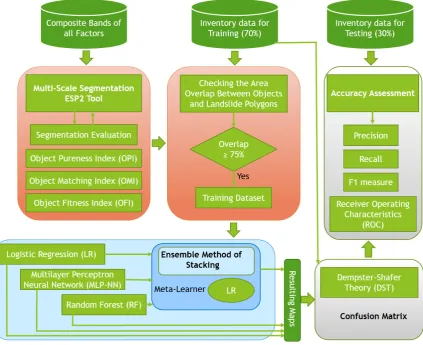
Moreover, to improve image classification and feature extraction, there are relevant probability concepts such as Dempster–Shafer theory (DST). The DST has been applied to classifier models to find the best match between the inventory data set and the resulting classification [31]. This probability concept has been used in RS data fusion [32] and landslide susceptibility mapping [33] to deal with uncertainty associated with the results. The DST has been successfully used for combining classifiers in a wide range of applications, such as target identification and object tracking [34,35]. In the field of landslide detection, Mezaal et al. [12] used the DST to enhance the results of the integration of OBIA with various ML methods, including SVM, random forest (RF), and K-nearest neighbor (KNN). The DST method performed well in landslide detection in their tropical study area. These pieces of evidence from previously published papers motivated us to apply the DST probability concept to improve the ML classification accuracy through integration with different classifiers. Therefore, in the present study, we integrate the widely used ML methods of logistic regression (LR), the multilayer perceptron neural network (MLP-NN), and RF with OBIA for landslide detection, based on optical data and topographic factors resulting from PlanetScope satellite images and Digital Elevation Model (DEM) data, respectively. To improve the performance of the applied ML methods, the ensemble method of stacking is used to combine them and produce a new result. The optimal scale for image segmentation is derived using the estimation of scale parameters (ESP2) tool [23]. Multiple scales are selected using interval values based on the optimal scale. The maps resulting from the multi-scale segmentation by each ML method are then fused using DST to demonstrate the advantages of working in a multi-scale environment. All resulting landslide detection maps are then validated using standard RS accuracy metrics and the validation method of receiver operating characteristics (ROC).

2. Study Area

In April 2015, an earthquake with a magnitude of 7.8 M struck Nepal, killing almost 9000 people and injuring nearly 22,000 [36]. The epicenter of the earthquake was located in the east of Gorkha district, and its hypocenter was at a depth of nearly 8.2 km [37]. Due to the magnitude of the earthquake, several landslides occurred across Nepal, especially in the east of the Gorkha district.

rough terrain, is very susceptible to landslide occurrence. According to the Köppen climate classification scheme, the study area falls under a sub-tropical and humid climate with cooler temperatures, and its annual average precipitation is nearly 691 mm. Before this study, some investigations by [38–40] and [1] were carried out to extract landslide locations in Rasuwa district. However, the main focus of the present study is evaluating the accuracy and performance of the proposed method of landslide detection compared to the conventional ML methods.

Remote Sens. 2019, 11, x FOR PEER REVIEW 4 of 28

temperatures, and its annual average precipitation is nearly 691 mm. Before this study, some investigations by [38–40] and [1] were carried out to extract landslide locations in Rasuwa district. However, the main focus of the present study is evaluating the accuracy and performance of the proposed method of landslide detection compared to the conventional ML methods.

Figure 1. The study area and a false color composite image of the orthorectified analytical scene of PlanetScope satellites and photographs of landslide events in Rasuwa district.

Remote Sens.2019,11, 2575 5 of 26

3. Methodology and Data

3.1. Overall Workflow

In this study, we used PlanetScope multispectral images [41] in four bands (Blue, Green, Red, and NIR), along with topographic factors, for landslide detection. The overall workflow (see Figure2) of this study is as follows:

I. Preparing multispectral images, the spectral index, and topographic derivatives for modeling; II. Generating multi-scale segments using the ESP2 tool and scale value intervals;

III. Segmentation analysis and evaluation;

IV. Training ML and stacking methods on multi-scale datasets at the object level; V. Fusing multi-scale ML results using DST;

VI. Applying different accuracy assessment metrics.

Remote Sens. 2019, 11, x FOR PEER REVIEW 5 of 28

3. Methodology and Data

3.1. Overall Workflow

In this study, we used PlanetScope multispectral images [41] in four bands (Blue, Green, Red, and NIR), along with topographic factors, for landslide detection. The overall workflow (see Figure 2) of this study is as follows:

I. Preparing multispectral images, the spectral index, and topographic derivatives for modeling;

II. Generating multi-scale segments using the ESP2 tool and scale value intervals; III. Segmentation analysis and evaluation;

IV. Training ML and stacking methods on multi-scale datasets at the object level; V. Fusing multi-scale ML results using DST;

VI. Applying different accuracy assessment metrics.

Figure 2. The flowchart of the applied methodology of the current study.

3.2. Datasets

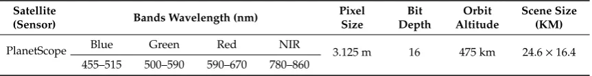
One of the most critical datasets for landslide detection and prediction is an appropriate landslide inventory, which influences further analyses [42,43]. In this case study, a landslide inventory map for the Rasuwa district was obtained from multiple sources, including GPS data from an extensive field survey and manually extracted data from satellite imagery. The satellite images used in this study were taken from the PlanetScope constellation of Planet Labs Company. PlanetScope includes more than 120 satellites that have been operating since 2014 and provide multispectral images with a 3 m spatial resolution and daily revisit time in four bands (Table 1). Due

Figure 2.The flowchart of the applied methodology of the current study. 3.2. Datasets

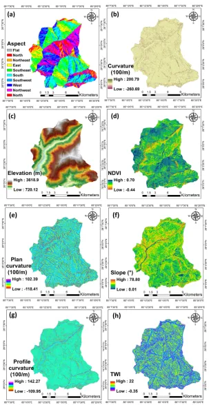
study area, some landslide events could not be registered by the field survey, so satellite images were used to identify and digitize them. Subsequently, all types of data were converted to the polygon format in QGIS 3.8. The total number and area of landslide events that were mapped were 194 and 64120 ha, respectively. Moreover, the minimum, maximum, and standard deviation of the area of the landslide polygons were 0.07, 16, and 2.17 ha, respectively. Along with PlanetScope images (Table1), the normalized difference vegetation index (NDVI) index—which is widely applied in landslide modeling [1,7,44]—was calculated from the NIR and Red bands to be used in landslide detection. Th probability of landslide occurrence is highly dependent on the surface topography; in other words, hilly and mountainous areas have the highest probability of landslide occurrence [1]. Our study area is located within the Himalayan fold and thrust zone of central Nepal. This zone resulted from a collision of the Indian Plate with the Eurasian plate. The precipitation amount of this area varies based on the tropical climatic conditions in the monsoon season, which has more rainfall compared to the summer season [45]. Although geological formations and precipitation are also important for landslide modeling, these factors do not change significantly in this study area due to its small size, which is why they were not considered in this study. Therefore, only satellite images and topographic factors were used, and all topographic derivatives, such as elevation, slope, aspect, curvature, and the topographic wetness index (TWI), were calculated based on a 5 m resolution DEM. The selection of topographical factors related to landslide occurrences depends on the landslide type, characteristics of the study area, and scale of the analysis. However, there is no standard approach for the selection of landslide conditioning factors. In the present study, six topographical landslide conditioning factors, namely, slope, slope aspect, curvature, plan and profile curvature, and altitude, were generated from a 5 m resolution DEM acquired from the Japanese aerospace exploration agency JAXA ALOS sensor.

Table 1.PlanetScope satellite sensor specifications.

Satellite

(Sensor) Bands Wavelength (nm)

Pixel Size

Bit Depth

Orbit Altitude

Scene Size (KM)

PlanetScope Blue Green Red NIR 3.125 m 16 475 km 24.6×_16.4

455–515 500–590 590–670 780–860

One of the most critical factors controlling slope stability is the slope angle. The slope angle is regularly used in landslide detection and susceptibility studies [46]. In the study area, the slope map was prepared using a DEM, and the slope ranged from 0.05◦to 75.26◦. The slope aspect was considered a topographical conditioning factor representing the slope direction [47]. The slope aspect factor mainly affects the hydrological system through evapotranspiration and, consequently, affects vegetation. Our aspect layer was classified, as this layer comprised sharp differences and changes. As such, the slope aspect of the area was divided into nine classes, namely, north, northwest, northeast, east, south, southeast, southwest, west, and flat.

We extracted the plane curvature from the DEM. The plane curvature represents the curvature of the contour line formed by the intersection of the surface with the horizontal plane [48]. The convergence and divergence of water in downhill flow are influenced by plane curvature [49]. The plane curvature represents the rate of change of aspect, in which positive values indicate convex curvature, zero denotes low change, and negative values indicate concave curvature. The values range from−_{56 to 74.14.}

The profile curvature is also crucial for the water flow speed variation from higher to lower areas [7]. The conditioning factor of altitude is another instability factor in our region, and landslide events at higher altitudes are usually influenced by gravity. Altitude influences topographical attributes and the Earth’s surface, which accounts for spatial variability in precipitation, soil thickness, erosion, and vegetation types [50]. In this study area, the elevation ranges from 734 to 4050 m above the mean sea level.

Remote Sens.2019,11, 2575 7 of 26

landslide and non-landslide areas. This index is useful for our study area, which is covered by forest. In this study, the NDVI map was derived from PlanetScope imagery from 28 November 2015 (see Equation (1)).

NDVI = (NIR−Red)

(NIR+Red) (1)

The NDVI was calculated from the near-infrared and the red spectral bands. The NDVI values vary from−_{0.44 to 0.72 in the study area.}

The TWI is another important topographical conditioning factor within the morphometric conditions of the terrain, as it evaluates the cumulative flow rate upstream with the slope angle [51]. The TWI is calculated by Equation (2):

TWI=ln (α/tanβ) (2)

whereαis the specific catchment area (m) andβis the slope. All conditioning factors are represented in Figure3.

3.3. Object-Based Image Analysis (OBIA)

3.3.1. Multi-Scale Image Segmentation

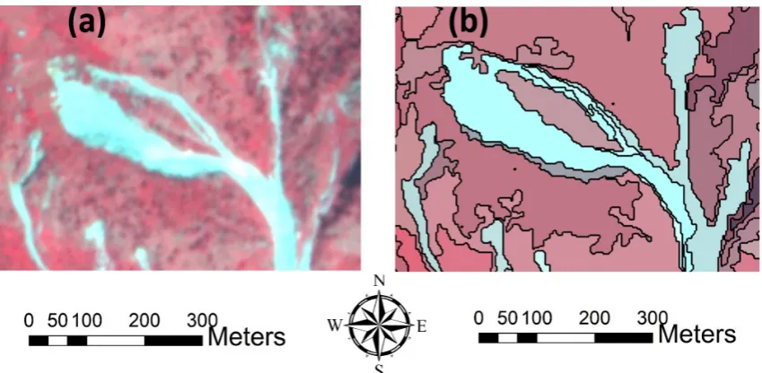
The demand for high-resolution (HR) and VHR satellite imagery, together with the resulting volume, variety, and velocity, as well as the rapid development and progress of EO technologies, provide significant challenges for the RS community with respect to the complexity of image understanding (IU) [52]. Therefore, OBIA, as an almost new paradigm in EO data analysis and image processing, has attracted more and more attention in the RS community and has been applied in several applications, such as image classification and object extraction [17]. OBIA is a knowledge-driven approach that aims to produce meaningful objects by using geometric and spectral characteristics, such as size, shape, texture, color, and contextual information, to present a better IU based on the real world [13]. In OBIA, segmentation is a crucial step [53], which considerably influences further analyses and results. The way that segmentation parameters (e.g., scale, shape, and compactness) are selected impacts the quality of the image objects [54]. In this study, multiresolution segmentation (MRS) was applied for the segmentation of our PlanetScope image (see Figure4). MRS is a bottom-up segmentation technique, which is based on the pairwise region-merging approach [12]. In this case, smaller detected objects were merged with larger ones, considering various parameters of scale, color, and shape (i.e., compactness and smoothness). These parameters are usually selected by trial-and-error, which requires expert knowledge and is a time-consuming and uncertain task [12,55]. Although some automatic techniques, like the Taguchi optimization method [55], have been introduced for defining the optimal parameters for the segmentation process, the process of detecting optimal objects is still a challenging task, mostly because of the diversity in the sizes and shapes of the target features [56].

In this regard, a variety of indices and metrics have been proposed, which are either area-based or location-based [22]. The accuracy of the segmentation using the selected scales was evaluated and presented in SectionRemote Sens. 2019, 11, x FOR PEER REVIEW 3.3.2. 8 of 28

Figure 3. Conditioning factors in landslide detection, including (a) aspect, (b) curvature, (c) elevation, (d) normalized difference vegetation index (NDVI), (e) plan curvature, (f) slope, (g) profile curvature, and topographic wetness index (TWI).

3.3. Object-Based Image Analysis (OBIA)

Remote Sens.2019,11, 2575 9 of 26

Remote Sens. 2019, 11, x FOR PEER REVIEW 10 of 28

Figure 4. Pseudo-color image of a landslide event (a) and segmented landslides (b).

3.3.2. Segmentation Accuracy Evaluation

Although we used the ESP2 tool to determine the optimal SP, there is no standard method to select segmentation parameters or assess the accuracy of the resulting objects [22]. The segmentation parameters are usually modified based on the desired target features, and they are challenging to implement and cannot appropriately address errors like under- and over-segmentation [22]. Therefore, we applied two indices that enabled us to evaluate the resulting objects using the multiresolution segmentation technique, along with the ESP2 tool and the corresponding interval values. These indices were the Object Pureness Index (OPI) on the one hand, and the Object Matching Index (OMI) on the other hand. OPI is a measure used to assess the integrity of the object in terms of spectral characteristics, and it is based on the standard deviation (SD) of multispectral bands because there is a robust positive correlation between the applied bands. The reason that SD is selected instead of each band’s mean value is that mean values vary among these bands, while SD values are very close to each other, especially for integrated objects like vegetated areas and water bodies. The other considered measure, OMI, evaluates the spatial match between the reference object and the image objects. The mathematical explanation of these measures is stated in Equation (3):

B G R

B G R

(SD + SD + SD )

(SD + SD + SD ) 3

OPI = =

Max SD 3 * Max SD

(3)

where SDB, SDG, and SDR stand for the SD of the Blue, Green, and Red bands, respectively, and Max

SD stands for the maximum SD value among these three bands. The OPI values close to 1 indicate that spectral variance is very low and the object is pure. In comparison, OPI values close to zero indicate that there is significant variance among the resulting objects, which usually happens when large-scale values are applied in the segmentation process. OPI alone is not adequate for selecting segmentation parameters, because it only evaluates objects in terms of spectral features, and does not address the spatial matching of objects. Therefore, the OMI (see Equation (4)) was also applied to evaluate our segmentation:

Area(R

S)

Area(S)

OMI =

Area(R)

Area(R)

∩

_×

(4)

where R is a reference object and S is a segmented object. An OMI value equal to 1 shows a perfect match between R and S, while values less than 1 indicate over-segmentation and values greater than 1 indicate under-segmentation. The Object Fitness Index (OFI) is calculated (as per Equation (5)) to

Figure 4.Pseudo-color image of a landslide event (a) and segmented landslides (b).

3.3.2. Segmentation Accuracy Evaluation

Although we used the ESP2 tool to determine the optimal SP, there is no standard method to select segmentation parameters or assess the accuracy of the resulting objects [22]. The segmentation parameters are usually modified based on the desired target features, and they are challenging to implement and cannot appropriately address errors like under- and over-segmentation [22]. Therefore, we applied two indices that enabled us to evaluate the resulting objects using the multiresolution segmentation technique, along with the ESP2 tool and the corresponding interval values. These indices were the Object Pureness Index (OPI) on the one hand, and the Object Matching Index (OMI) on the other hand. OPI is a measure used to assess the integrity of the object in terms of spectral characteristics, and it is based on the standard deviation (SD) of multispectral bands because there is a robust positive correlation between the applied bands. The reason that SD is selected instead of each band’s mean value is that mean values vary among these bands, while SD values are very close to each other, especially for integrated objects like vegetated areas and water bodies. The other considered measure, OMI, evaluates the spatial match between the reference object and the image objects. The mathematical explanation of these measures is stated in Equation (3):

OPI =

(SD_B+SDG+SDR)

3

Max SD =

(SD_B+SDG+SDR)

3 ∗ _{Max SD} (3)

where SDB, SDG, and SDRstand for the SD of the Blue, Green, and Red bands, respectively, and Max SD stands for the maximum SD value among these three bands. The OPI values close to 1 indicate that spectral variance is very low and the object is pure. In comparison, OPI values close to zero indicate that there is significant variance among the resulting objects, which usually happens when large-scale values are applied in the segmentation process. OPI alone is not adequate for selecting segmentation parameters, because it only evaluates objects in terms of spectral features, and does not address the spatial matching of objects. Therefore, the OMI (see Equation (4)) was also applied to evaluate our segmentation:

OMI = Area(R∩S) Area(R) ×

Area(S)

Area(R) (4)

obtain a single index that can present the optimal object generation scale based on OPI and OMI, among other scales:

OFI =

r

(OPI

2_+OMI2

2 ) (5)

OFI values close to 1 point to the optimal segmentation scale. Resulting values less and greater than 1 indicate over- and under-segmentation, respectively.

3.4. Machine Learning Methods

3.4.1. Multilayer Perceptron Neural Network (MLP-NN)

ML algorithms have been widely used in various scientific fields, especially in the earth sciences, to overcome complex problems [58,59]. ML is considered a subdivision of artificial intelligence, which imitates the human brain’s performance in problem-solving and decision making [60]. In doing so, it uses a variety of algorithms, like artificial neural network (ANN), in the learning process [59]. MLP-NN is an ANN method that has been widely used in geohazard modeling [1]. The performance of this method is affected by variables like the model’s structure, the type of applied activation functions, and which weight updating method is used [61]. In general, MLP-NN consists of an input layer, one or more hidden layers, and an output layer. In geohazard modeling, like landslide susceptibility modeling, the input layer includes neurons that are the same as the landslide affecting factors, and the number of hidden layers depends on the training data [62] and the complexity of the problem [1]. In this study, the backpropagation algorithm (BPA), which is the primary training method employed in neural networks, was used for updating weights; for two hidden layers, 24 neurons for each layer were allocated. To run the method, initial weights, which are randomly chosen by the BPA, are allocated to each neuron, and the method is then continually optimized based on the error rate between the output and expected values until the error rate is stabilized (see Equation (6)):

y= (

n X

i=1

Wi∗Xi+b) (6)

whereWdenotes the vector of weights,Xis the input vector of features of objects, andbis the bias. Additionally, the sigmoid activation function, which was used in the present study, can be explained by Equation (7):

f (z) = 1

1−_e−_y, (7)

wheref (z) is the output of the activation function, which ranges from 0 to 1.

3.4.2. Logistic Regression (LR)

Logistic regression is one of the multivariate analysis methods that allow us to create a multivariate regression connection among a set of independent variables and one dependent variable [63]. LR is a powerful method for predicting the presence of an event by fitting the best linear model based on independent variable values, and it is a commonly used statistical method applied in landslide susceptibly analysis [64]. One of the significant advantages of LR is that, in this method, the independent variables can be both discrete and continuous, or a mix of these variable types can be used [65]. In this case, the dependent variable was introduced as a binary value of 0 and 1, whereby 0 showed the absence of a landslide event and 1 indicated the presence of a landslide. The mathematical definition of LR is defined by Equation (8) [63]:

p = 1

Remote Sens.2019,11, 2575 11 of 26

where p, in this case, is the probability of a landslide occurring, which varies between 0 and 1. Furthermore, z is the linear combination, which fits a linear equation to independent variables (landside conditioning factors), as shown by Equation (9) [63]:

z = b0+b1x1+b2x2+b3x3+. . .+bnxn (9)

whereb0,bi, andxiare intercepts of the method, coefficient, and independent variables, respectively.

3.4.3. Random Forest (RF)

RF is a powerful supervised ML method, which was proposed by [66] and has been widely used in RS and GIS applications, such as image classification [67] and landslide susceptibility mapping [1]. This method is based on decision trees and operates by constructing a multitude of decision trees during the training process, which makes it less sensitive to over-fitting issues [1]. In the RF method, each decision tree generates outputs, and then outputs weights, which are derived from the votes, are dedicated. The advantages of RF are that it is easy to apply because it requires fewer parameters and it yields a higher accuracy compared to other ML methods due to the bagging process [68]. Additionally, it can deal with high-dimensional and complex data structures [69]. Due to its simplicity and better performance, we selected this method as another algorithm for landslide detection in this study.

3.4.4. Stacking Machine Learning (ML) Methods

The main idea behind ensemble methods in ML is to improve the performance of a final method, by combining various methods to build a powerful learner to predict or classify a set of data [70]. The strength of using ensemble methods is that we can decrease the variance by combining several single methods, which, individually, do not yield an excellent performance [70]. There are three main ensemble machine learning methods: bagging, boosting, and stacking. In this case, the stacking method was used. In stacking, there are two levels, namely, level 0 and level 1. In level 0, single methods make a set of predictions based on training data, and these outputs (predictions) are then used as inputs for a meta-learner, which is a single method, to make a new set of predictions [71]. Therefore, in this case, ML methods such as LR, MLP-NN, and RF were trained as single methods in level 0, and LR was then used as our meta-learner in level 1 to make the final predictions.

3.5. Integration of MLP-NN and OBIA for Landslide Detection

3.6. Dempster–Shafer Theory (DST)

The concept of DST is made based on a frame of discernment and known as a belief function (Bel) that is derived from Bayesian probability theory (BPT). It obtained its name from the extensions and clarifications presented by Shafer and is considered a great approach to integrating spatial data [72]. The DST is an effective method for modeling imprecision and uncertainty assessment. The DST is transformed from events to proposition and an event set to proposition set, which defines the concept of the basic probability assignments (bpa) function, Bel, and the plausibility function (Pl), and determines the one-to-one relationship of proposition and set. Therefore, the DST can translate the proposition uncertainty into a set uncertainty [73]. In this theory, displaying information requires two essential functions, namely, Bel and the Pl, which derive the lower bound value for a known probability function and the upper bound value for an unknown probability function. The differentiation between Bel and Pl illustrates the uncertainty of the knowledge about the objective proposition.

The DST provides an extension of the probability framework for assessing the uncertainty of any imprecision event of the probabilityP(Ml) that the alternative methodMl,l=1, ...,nis correct.

The lower bound indicates the degree of knowledge or belief that supports Mland represents Bel (Ml).

In comparison, the upper bound indicates the probability ofMl, and is called plausibilityPl(Ml) [74]

(see the Equations (10) and (11)):

Bel(A) =X

B⊆_A

m(B) (10)

Pl(A) = X

B∩A,0

m(B) (11)

where the summation is obtained over all setsB∈ ₂8 _withB ⊆ _{Ain the definition of Bel and the}

summation in that of Pl is taken over allB∈ ₂8 _{with B}∩_{A , 0 in which the set of} 8is mutually exclusive and collectively exhaustive hypotheses, and the power set of8is denoted by 28. The Bel is the summation of all masses directly assigned by a set of hypothesisA, while the plausibility sums all masses not assigned to the complement of the hypothesisA. An uncertainty interval of_Bel(A),Pl(A)

thatBel(A)≤_{Pl(A) can be defined; its length is a measure of the imprecision of knowledge about the}

uncertainty of setA[75].

From a general point of view, unlike a probabilistic theory that allocates a mass to the individual elementary events, the theory of evidence, or the bpa, makesm(A) on the setAof theP(z), power sets of the spaceZevent, i.e., on a set of results rather than a single elementary event.

In more detail,m(A) expresses the degree of belief that a specific element x belongs to the setA only, and not to any subset ofA. The bpa that assigns a mass in the range of [0, 1] to each subsetA satisfies the following requirement, specified by Equation (12):

m : P(z) → _{[0, 1], m(φ) = 0;}X A∈_Z

m(A) =1 (12)

Ifndata sources are available, probability massesmi(Bj) must be defined for each data sourcei

with1≤_i≤_{n and for all sets,Bj}∈₂8_{. The DST allows the combination of these probability masses}

from resulting landslide detection maps and the training inventory data set to compute a combined probability mass for each set. The composition rule in the proposed DST is based on mathematical theory, which is the basis of the combination of mass functionsmiobtained fromnsources of information

given in Equations (13) and (14):

m(A) =m1(B1)⊕m2(B2)⊕M3(B3). . . . ⊕ mn(Bn) (13)

m(A) =

P

B1∩B2....Bn=A Qn

i=1mi

Bj

Remote Sens.2019,11, 2575 13 of 26

whereKdenotes the degree of conflict given in Equation (15):

K = X

B1∩B2....Bn=ϕ n Y

i=1 mi

Bj

(15)

Fusion of Multi-Scale Results via DST

Multi-scale segmentation resulted in different object sizes, which were used for training the ML methods. Therefore, based on multi-scale segmentation, different landslide detection maps were produced from each ML method. The areas that were classified as landslides using different scales and one ML method were grouped by the fusion level analysis (FLA) technique [12] and fused into a class of landslide area based on the DST. Several Bels were combined in the DST within the same frame, which made it possible to harmonize the landslide detected areas from different scales. The probability of uncertainty in the detected landslide areas can be derived from Bel and Pl. Therefore, the resulting areas detected as landslides in three scales (i.e., 198, 248, and 298) were combined by fusing the DST with the training inventory dataset. The accuracy of the landslide detected areas based on each scale was assessed using a confusion matrix and, accordingly, the Bels were estimated by a precision function [12]. The DST combined the majority of landslide detected areas, which were closer to the inventory dataset, and then assigned them to the class of landslide area based on the DST.

4. Accuracy Assessment and Comparison

In this section, we outline the most common accuracy assessment methods, which were used to validate the performance of the applied ML methods and the improvements made by using the stacking and DST methods. The accuracy assessment was made by comparing the resulting landslide detection maps with the landslide inventory dataset. The accuracy assessment was conducted using a confusion matrix, precision, recall F1 measure, and the receiver operating characteristics (ROC), to determine the accuracy of the landslides detected by each method. The user accuracy was calculated based on dividing correctly mapped objects by the total number of classified objects. In this regard, the study area was divided into two classes called landslide areas and non-landside areas, and for each class, this measure was calculated. We used the confusion matrix based on a comparison of the inventory dataset and the resulting maps based on a pixel-based environment. The Kappa coefficient was derived from the confusion matrix [76], and the coefficient was calculated using Equation (16):

Kappa Coefficient = (θ1− θ2)/(1− θ2) (16)

whereθ1denotes the ratio of correctly detected areas, whereasθ2denotes the proportion of agreement by randomness [12].

The ROC is a graphical plot used to evaluate the validity of a method that predicts the location of the occurrence of events by comparing the probabilistic map of the event with a reference map [77]. This assessment method has been applied in many fields, in particular, in the Geosciences [78]. The ROC measure is based on three metrics: true positive (TP), false positive (FP), and false-negative (FN) (see Figure5and Equations (17)–(19)). In this case, the landslide events that were correctly detected were TPs, areas that were incorrectly classified as landslides were FPs, and FNs represented landslide areas that were not detected. Using these metrics, the three parameters of Precision, Recall, and F1 measure could be calculated to assess the results. Precision shows the proportion of landslide events that were detected, Recall indicates how many of the inventory landslide events were detected, and the F1 measure was used to balance the Precision and Recall.

Precision = TPs

Recall = TPs

TPs+FNs (18)

F1 meausre = 2 × Precision × Recall

Precision + Recall (19)

Remote Sens. 2019, 11, x FOR PEER REVIEW 15 of 28

Precision Recall

F1 meausre = 2

Precision + Recall

×

×

Figure 5. Illustration of accuracy assessment measures.

5. Results and Discussion

5.1. Image Segmentation

The MRS parameters and results of ten applied scales were chosen by interval values based on the ESP2 tool scale value of 248. The NDVI and topographic derivatives, along with PlanetScope images, were used as the conditioning factors in our image segmentation procedure, to improve the segmentation results. Next, to evaluate the accuracy of our segmentation results, 30% of the inventory dataset of landslide events were randomly selected for use in the OPI, OFI, and OMI indices. The applied parameters and layer weights, and the segmentation evaluation results are presented in Table 2.

Table 2. Parameters used for the multiresolution segmentation (MRS) and segmentation evaluation results.

Scale Shape Compactness

Layer Weights OPI OMI OFI

RGB NIR

TWI _{aspect profile}

curvature elevation NDVI slo

p

e

curvature

plan curvature

48 0.7 0.3 0.88 0.40 0.68

98 0.7 0.3 0.93 0.51 0.75

148 0.7 0.3 0.95 0.71 0.84

198 0.7 0.3 0.95 0.87 0.91

248 0.7 0.3 2 1 2 1 1 4 2 1 1 0.97 0.95 0.96

298 0.7 0.3 0.94 1.19 1.07

348 0.7 0.3 0.92 1.25 1.10

398 0.7 0.3 0.90 1.29 1.11

448 0.7 0.3 0.87 1.35 1.14

498 0.7 0.3 0.81 1.41 1.15

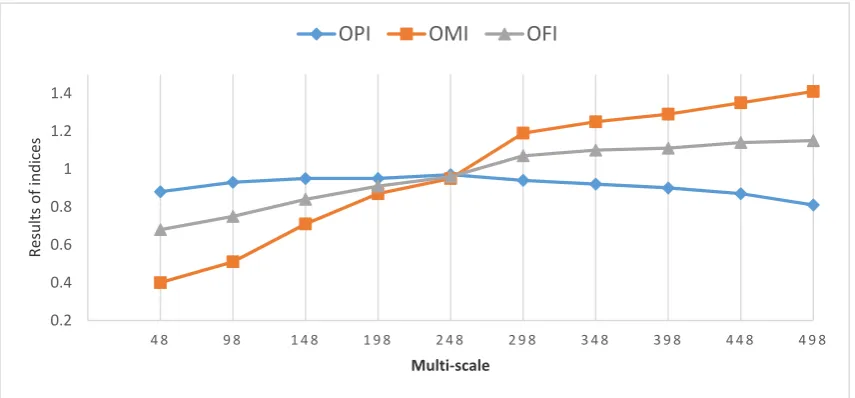
For the accuracy assessment of our segmentation results, we selected image objects whose centroids were within the reference objects. According to Table 2, based on the OFI index results of 30% of the applied samples, the segmentation with a scale of 248 provides the best convergence, while

Figure 5.Illustration of accuracy assessment measures.

5. Results and Discussion

5.1. Image Segmentation

The MRS parameters and results of ten applied scales were chosen by interval values based on the ESP2 tool scale value of 248. The NDVI and topographic derivatives, along with PlanetScope images, were used as the conditioning factors in our image segmentation procedure, to improve the segmentation results. Next, to evaluate the accuracy of our segmentation results, 30% of the inventory dataset of landslide events were randomly selected for use in the OPI, OFI, and OMI indices. The applied parameters and layer weights, and the segmentation evaluation results are presented in Table2.

Table 2. Parameters used for the multiresolution segmentation (MRS) and segmentation evaluation results.

Scale Shape Compactness

Layer Weights OPI OMI OFI RGB

NIR TWI aspect Profile

CurvatureElevation NDVI Slope Curvature Plan Curvature

48 0.7 0.3 0.88 0.40 0.68

98 0.7 0.3 0.93 0.51 0.75

148 0.7 0.3 0.95 0.71 0.84

198 0.7 0.3 0.95 0.87 0.91

248 0.7 0.3 2 1 2 1 1 4 2 1 1 0.97 0.95 0.96

298 0.7 0.3 0.94 1.19 1.07

348 0.7 0.3 0.92 1.25 1.10

398 0.7 0.3 0.90 1.29 1.11

448 0.7 0.3 0.87 1.35 1.14

498 0.7 0.3 0.81 1.41 1.15

Remote Sens.2019,11, 2575 15 of 26

due to a small SP, the landslide event is over-segmented, while in Figure7c, the scale is relatively large, resulting in under-segmentation, which merged a non-landslide area with a landslide area. Figure7b shows the best segmentation result compared to other scales. The main reason that three scale results are used for landslide detection is to evaluate the impact of different scales on the landslide detection accuracy. Since, in OBIA, processing units are image objects, other features (e.g., geometric, textural, and spectral) of objects can be calculated and used in the classification or object extraction. Therefore, in this case, we calculated characteristics such as the shape index, mean brightness, SD of NDVI, length, compactness, density, and contrast grey level of the co-occurrence matrix (GLCM), to be used in MLP-NN algorithms. In order to train MLP-NN for each segmentation result, the objects that overlapped with training data (polygons) were chosen as training objects. Subsequently, the trained algorithm was applied to test objects.

Remote Sens. 2019, 11, x FOR PEER REVIEW 16 of 28

scales lower and higher than scale 248 are associated with over-segmentation and under-segmentation errors, respectively. The variation of the resulting values from OPI, OMI, and OFI are shown in Figure 6. The segmentation results in Figure 7 show the over- and under-segmentation errors. In Figure 7a, due to a small SP, the landslide event is over-segmented, while in Figure 7c, the scale is relatively large, resulting in under-segmentation, which merged a non-landslide area with a landslide area. Figure 7b shows the best segmentation result compared to other scales. The main reason that three scale results are used for landslide detection is to evaluate the impact of different scales on the landslide detection accuracy. Since, in OBIA, processing units are image objects, other features (e.g., geometric, textural, and spectral) of objects can be calculated and used in the classification or object extraction. Therefore, in this case, we calculated characteristics such as the shape index, mean brightness, SD of NDVI, length, compactness, density, and contrast grey level of the co-occurrence matrix (GLCM), to be used in MLP-NN algorithms. In order to train MLP-NN for each segmentation result, the objects that overlapped with training data (polygons) were chosen as training objects. Subsequently, the trained algorithm was applied to test objects.

Figure 6. Changes of the object pureness index (OPI), object matching index (OMI), and object fitness index (OFI) at different scales. Scale 248, where all lines cross, turned out to be the best segmentation scale.

Figure 7. Image segmentation with different results; the black colored area represents a landslide event, and blue polygons are image objects. Images (a–c) are segmentation results with scales of 198, 248, and 298, respectively.

0.2 0.4 0.6 0.8 1 1.2 1.4

4 8 9 8 1 4 8 1 9 8 2 4 8 2 9 8 3 4 8 3 9 8 4 4 8 4 9 8

Re

sults of indice

s

Multi-scale

OPI

OMI

OFI

Figure 6. Changes of the object pureness index (OPI), object matching index (OMI), and object fitness index (OFI) at different scales. Scale 248, where all lines cross, turned out to be the best segmentation scale.

Remote Sens. 2019, 11, x FOR PEER REVIEW 16 of 28

scales lower and higher than scale 248 are associated with over-segmentation and under-segmentation errors, respectively. The variation of the resulting values from OPI, OMI, and OFI are shown in Figure 6. The segmentation results in Figure 7 show the over- and under-segmentation errors. In Figure 7a, due to a small SP, the landslide event is over-segmented, while in Figure 7c, the scale is relatively large, resulting in under-segmentation, which merged a non-landslide area with a landslide area. Figure 7b shows the best segmentation result compared to other scales. The main reason that three scale results are used for landslide detection is to evaluate the impact of different scales on the landslide detection accuracy. Since, in OBIA, processing units are image objects, other features (e.g., geometric, textural, and spectral) of objects can be calculated and used in the classification or object extraction. Therefore, in this case, we calculated characteristics such as the shape index, mean brightness, SD of NDVI, length, compactness, density, and contrast grey level of the co-occurrence matrix (GLCM), to be used in MLP-NN algorithms. In order to train MLP-NN for each segmentation result, the objects that overlapped with training data (polygons) were chosen as training objects. Subsequently, the trained algorithm was applied to test objects.

Figure 6. Changes of the object pureness index (OPI), object matching index (OMI), and object fitness index (OFI) at different scales. Scale 248, where all lines cross, turned out to be the best segmentation scale.

Figure 7. Image segmentation with different results; the black colored area represents a landslide event, and blue polygons are image objects. Images (a–c) are segmentation results with scales of 198, 248, and 298, respectively.

0.2 0.4 0.6 0.8 1 1.2 1.4

4 8 9 8 1 4 8 1 9 8 2 4 8 2 9 8 3 4 8 3 9 8 4 4 8 4 9 8

Re

sults of indice

s

Multi-scale

OPI

OMI

OFI

5.2. Landslide Detection using ML and Stacking Methods

The training image objects of each segmentation scale, along with their characteristics, were stored in a CSV file to train ML methods in the Python environment. Results for all scales vary between 0 and 1, and objects that had values greater than 0.5 were selected as landslide events for all ML methods. The results in Figure8show that the size of objects has a significant impact on the outputs. For example, the results of ML and stacking methods of image objects with a scale of 298 indicate larger areas as landslides than the other scales’ results. However, based on the OPI and OMI indices, differences in the results were expected, because the OPI and OMI values of scales 198 and 248 are close to each other and are associated with an over-segmentation error. Meanwhile, for the scale 298, the values of those indices—OMI, in particular—show an under-segmentation error, which resulted in larger image objects. Additionally, the methods’ parameters were the same for each segmentation scale.Remote Sens. 2019, 11, x FOR PEER REVIEW 18 of 28

Figure 8. Results of different machine learning (ML) methods, stack, and Dempster–Shafer theory (DST) using multi-scale segmentation.

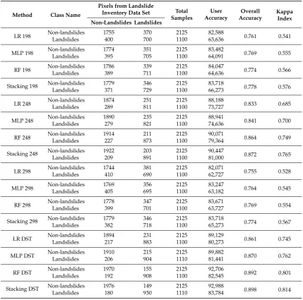
According to the results, which are represented in Table 3, the RF method achieved the highest user accuracy of all ML methods, with an accuracy of up to 90.07% when detecting non-landslides using the optimal SP. This resulting accuracy was followed by the MLP-NN and LR methods, with almost an 89% and 88.2% accuracy, respectively, again using the optimal SP. For this SP, the stacking method slightly improved the user accuracy to 90.44%. However, combining multi-scale results using the DST increased the user accuracy for all applied methods by up to 9%.

Remote Sens.2019,11, 2575 17 of 26

5.3. Results of Fusion and Optimization using DST

To optimize the landslide detection using the ML method and obtain the best result, we used DST to combine the results of each method’s landslide detection output at different scales. Therefore, the predicted landslides acquired from each method were calculated using a confusion matrix, and a CSV file was employed to fuse the most probable landslide events in QGIS 3.8, which resulted in a single and accurate landslide inventory map for each method (Figure8).

According to the results, which are represented in Table3, the RF method achieved the highest user accuracy of all ML methods, with an accuracy of up to 90.07% when detecting non-landslides using the optimal SP. This resulting accuracy was followed by the MLP-NN and LR methods, with almost an 89% and 88.2% accuracy, respectively, again using the optimal SP. For this SP, the stacking method slightly improved the user accuracy to 90.44%. However, combining multi-scale results using the DST increased the user accuracy for all applied methods by up to 9%.

Table 3.Confusion matrices based on different methods and the landslide inventory data set.

Method Class Name

Pixels from Landslide

Inventory Data Set Total Samples

User Accuracy

Overall Accuracy

Kappa Index Non-Landslides Landslides

LR 198 Non-landslides 1755 370 2125 82,588 0.761 0.541

Landslides 400 700 1100 63,636

MLP 198 Non-landslides 1774 351 2125 83,482 0.769 0.555

Landslides 395 705 1100 64,091

RF 198 Non-landslides 1786 339 2125 84,047 0.774 0.566

Landslides 389 711 1100 64,636

Stacking 198 Non-landslides 1779 346 2125 83,718 0.778 0.576

Landslides 371 729 1100 66,273

LR 248 Non-landslides 1874 251 2125 88,188 0.833 0.685

Landslides 289 811 1100 73,727

MLP 248 Non-landslides 1890 235 2125 88,941 0.841 0.700

Landslides 279 821 1100 74,636

RF 248 Non-landslides_Landslides 1914₂₂₇ 211₈₇₃ 2125₁₁₀₀ 90,071_79,364 0.864 0.749

Stacking 248 Non-landslides_Landslides 1922₂₀₉ 203₈₉₁ 2125₁₁₀₀ 90,447_81,000 0.872 0.765

LR 298 Non-landslides_Landslides 1744₄₁₀ 381₆₉₀ 2125₁₁₀₀ 82,071_62,727 0.755 0.528

MLP 298 Non-landslides 1769 356 2125 83,247 0.764 0.545

Landslides 405 695 1100 63,182

RF 298 Non-landslides 1778 347 2125 83,671 0.769 0.554

Landslides 399 701 1100 63,727

Stacking 298 Non-landslides 1779 346 2125 83,718 0.774 0.567

Landslides 382 718 1100 65,273

LR DST Non-landslides 1894 231 2125 89,129 0.861 0.745

Landslides 217 883 1100 80,273

MLP DST Non-landslides 1910 215 2125 89,882 0.870 0.762

Landslides 206 904 1110 81,441

RF DST Non-landslides 1970 155 2125 92,706 0.892 0.801

Landslides 192 908 1100 82,545

Stacking DST Non-landslides 1976 149 2125 92,988 0.898 0.814

Landslides 180 930 1110 83,784

values close to 0.5 show a method’s poor performance. Table4presents the quantitative assessment accuracy of each method based on the testing inventory dataset. The ROC validation results showed that the DST-stacking results achieved the highest AUC value of 0.965, whereas the LR method, based on the scale of 180 with an AUC value of 0.88, presented the lowest accuracy in landslide detection (see Figure9and Table5). Furthermore, for each result, the precision, recall, and F1 measures were also calculated.

Table 4.Quantitative accuracy assessment for ML and Stacking methods, as well as DST results.

Method Scale TP (ha) FP (ha) FN (ha) Precision Recall F1 Measure

LR

198 572.89 344.72 68.24 0.62 0.89 0.74

248 553.39 272.62 87.74 0.67 0.86 0.75

298 570.65 532.20 70.48 0.52 0.89 0.65

MLP

198 598.96 310.09 42.17 0.66 0.93 0.77

248 580.04 220.00 61.09 0.73 0.90 0.80

298 580.47 479.65 60.66 0.55 0.91 0.68

RF

198 579.54 265.76 61.59 0.69 0.90 0.78

248 588.54 140.23 52.59 0.81 0.92 0.86

298 608.44 419.65 32.69 0.59 0.95 0.73

Stacking

198 580.30 131.23 60.83 0.82 0.91 0.86

248 594.25 109.23 46.88 0.84 0.93 0.88

298 591.52 289.60 49.61 0.67 0.92 0.78

DST

LR 589.74 84.25 51.39 0.87 0.92 0.90

MLP 594.36 74.44 46.77 0.89 0.93 0.91

RF 604.15 55.85 36.98 0.92 0.94 0.93

Stacking 616.06 11.93 25.07 0.98 0.96 0.97

Remote Sens. 2019, 11, x FOR PEER REVIEW 20 of 28

Stacking

198 580.30 131.23 60.83 0.82 0.91 0.86

248 594.25 109.23 46.88 0.84 0.93 0.88

298 591.52 289.60 49.61 0.67 0.92 0.78

DST

LR 589.74 84.25 51.39 0.87 0.92 0.90

MLP 594.36 74.44 46.77 0.89 0.93 0.91

RF 604.15 55.85 36.98 0.92 0.94 0.93

Stacking 616.06 11.93 25.07 0.98 0.96 0.97

Figure 9. Receiver operating characteristics (ROC) analysis and area under the curve (AUC) values for ML, Stacking, and DST results.

Table 5. The accuracy assessment results based on the area under the curve (AUC).

Scale LR MLP RF Stack

198 0.88 0.92 0.93 0.94 248 0.91 0.92 0.94 0.95 298 0.89 0.9 0.91 0.92 DST 0.93 0.93 0.94 0.96

To visually present the improvement of the results using the optimal scale, stacking, and DST, we enlarged a specific area of a landslide event (see Figure 10). This figure illustrates that the ML and stacking results based on objects at a scale of 298 are much more prone to FPs. Although the multi-scale approach resulted in different TP, FP, and FN areas, the DST was helpful for merging the TP areas of different scales and considerably improved the landslide detection accuracy. For instance, the result of stacking at a scale of 298 resulted in considerably more FPs, but this was not the case for the other scale levels, namely 248 and 198. However, as the DST combined the majority of TP areas, the FPs of the scale 298 were removed from the DST results.

Remote Sens.2019,11, 2575 19 of 26

Table 5.The accuracy assessment results based on the area under the curve (AUC).

Scale LR MLP RF Stack

198 0.88 0.92 0.93 0.94

248 0.91 0.92 0.94 0.95

298 0.89 0.9 0.91 0.92

DST 0.93 0.93 0.94 0.96

To visually present the improvement of the results using the optimal scale, stacking, and DST, we enlarged a specific area of a landslide event (see Figure10). This figure illustrates that the ML and stacking results based on objects at a scale of 298 are much more prone to FPs. Although the multi-scale approach resulted in different TP, FP, and FN areas, the DST was helpful for merging the TP areas of different scales and considerably improved the landslide detection accuracy. For instance, the result of stacking at a scale of 298 resulted in considerably more FPs, but this was not the case for the other scale levels, namely 248 and 198. However, as the DST combined the majority of TP areas, the FPs of the scale 298 were removed from the DST results.

Figure 10. Enlarged maps showing the capabilities of DST to reduce both false positive and false negative areas in landslide detection through multi-scale ML and stacking methods.

Remote Sens.2019,11, 2575 21 of 26

Remote Sens. 2019, 11, x FOR PEER REVIEW 23 of 28

Figure 11. Changes of AUC, precision, recall, and F1 measure values for each method and scale.

6. Conclusions

We have developed a methodology that incorporates OBIA with three machine learning methods, namely, logistic regression (LR), the multilayer perceptron neural network (MLP-NN), and random forest (RF), for landslide detection. Our multi-scale methodology identifies the optimal scale parameters (SP) and uses them for multi-scale segmentation and further analysis. The presented landslide mapping study showed that the integrated method improves the performance and accuracy. Most notably, the stacking method for landslide detection outperformed every single ML method. Furthermore, the validation results show that using DST could optimize and improve the outcomes of all applied methods. However, it should be noted that the results of an object-based ML method strongly depend on the segmentation quality. Therefore, optimal segmentation parameters result in a higher segmentation accuracy and, consequently, better results. Although there are no standard methods for selecting segmentation parameters and for accuracy assessment, we used the two measures of OPI and OMI to identify ideal segmentation parameters in terms of spectral and spatial quality. Therefore, as a result, both measures were combined to create the OFI, which allowed us to identify the best segmentation parameters, as well as to identify over-segmentation and under-segmentation errors. Therefore, we believe that a challenge for object-based ML methods is improving the segmentation accuracy, which requires new reliable automatic methods dealing with intra-class heterogeneity and inter-class homogeneity. This study shows that using high-resolution satellite imagery data does not guarantee a good accuracy. Several measures and parameters should be identified based on the target object detection or classification. In this regard, we used an ensemble method of stacking and DST to enhance the landslide detection results based on multi-scale segmentation. Different accuracy assessment results proved that the performance of landslide detection can be increased using these two methods. Moreover, all resulting maps yielded the highest accuracies using the optimal SP. Therefore, finding the optimal SP for the applied satellite image and ML method for the classification is crucial for accurate landslide detection. Based on the results of the present study, our future work will focus more on improving both segmentation and classification using relative mathematical and probability concepts, such as the central limit theorem (CLT) and fuzzy set theory (FST).

Author Contributions: conceptualization, S.T.P., H.S. and O.G.; methodology, S.T.P., H.S. and K.G.; validation, S.T.P., H.S.; formal analysis, S.T.P. and H.S.; data curation, S.R.M.; writing—original draft preparation, S.T.P., H.S., O.G. and S.R.M.; writing—review and editing, B.J., T.B. and J.A.; visualization, H.S., O.G and S.R.M; supervision, T.B. and J.A.; funding acquisition, T.B.

Funding: This research is partly funded by the Austrian Science Fund (FWF) through the GIScience Doctoral College (DK W 1237-N23).

0 0.2 0.4 0.6 0.8 1 1.2

Accur

acy

ML methods, stack, and DST using multi-scale

AUC

Precision

Recall

F1 measure

Figure 11.Changes of AUC, precision, recall, and F1 measure values for each method and scale.

6. Conclusions

We have developed a methodology that incorporates OBIA with three machine learning methods, namely, logistic regression (LR), the multilayer perceptron neural network (MLP-NN), and random forest (RF), for landslide detection. Our multi-scale methodology identifies the optimal scale parameters (SP) and uses them for multi-scale segmentation and further analysis. The presented landslide mapping study showed that the integrated method improves the performance and accuracy. Most notably, the stacking method for landslide detection outperformed every single ML method. Furthermore, the validation results show that using DST could optimize and improve the outcomes of all applied methods. However, it should be noted that the results of an object-based ML method strongly depend on the segmentation quality. Therefore, optimal segmentation parameters result in a higher segmentation accuracy and, consequently, better results. Although there are no standard methods for selecting segmentation parameters and for accuracy assessment, we used the two measures of OPI and OMI to identify ideal segmentation parameters in terms of spectral and spatial quality. Therefore, as a result, both measures were combined to create the OFI, which allowed us to identify the best segmentation parameters, as well as to identify over-segmentation and under-segmentation errors. Therefore, we believe that a challenge for object-based ML methods is improving the segmentation accuracy, which requires new reliable automatic methods dealing with intra-class heterogeneity and inter-class homogeneity. This study shows that using high-resolution satellite imagery data does not guarantee a good accuracy. Several measures and parameters should be identified based on the target object detection or classification. In this regard, we used an ensemble method of stacking and DST to enhance the landslide detection results based on multi-scale segmentation. Different accuracy assessment results proved that the performance of landslide detection can be increased using these two methods. Moreover, all resulting maps yielded the highest accuracies using the optimal SP. Therefore, finding the optimal SP for the applied satellite image and ML method for the classification is crucial for accurate landslide detection. Based on the results of the present study, our future work will focus more on improving both segmentation and classification using relative mathematical and probability concepts, such as the central limit theorem (CLT) and fuzzy set theory (FST).

Author Contributions:conceptualization, S.T.P., H.S. and O.G.; methodology, S.T.P., H.S. and K.G.; validation, S.T.P., H.S.; formal analysis, S.T.P. and H.S.; data curation, S.R.M.; writing—original draft preparation, S.T.P., H.S., O.G. and S.R.M.; writing—review and editing, B.J., T.B. and J.A.; visualization, H.S., O.G. and S.R.M.; supervision, T.B. and J.A.; funding acquisition, T.B.

Acknowledgments:Authors thank PlanetScope for providing satellite images. We also thank ALOS for providing Digital Elevation Data. We also would like to thank autonomous reviewers for their constructive inputs on the manuscript. OpenAccess Funding by the Austrian Science Fund (FWF).

Conflicts of Interest:The authors declare no conflict of interest.

Abbreviations

AUC area under the curve

BPA backpropagation algorithm

BPT Bayesian probability theory bpa basic probability assignments

Bel belief function

CSV comma separate values

CLT central limit theorem

DST Dempster–Shafer theory

DEM digital elevation model

DN digital number

EO Earth observation

ESP2 estimation of scale parameters EBF evidential belief function

FP false positive

FN false negative

FST fuzzy set theory

FLA fusion level analysis

GPS global positioning system

GIS geographic information system

GIScience geographic information science GLCM grey level co-occurrence matrix

HR high-resolution

IU image understanding

LR logistic regression

KNN K-nearest neighbour

LMT logistic model tree

MSL mean sea level

MLP-NN multilayer perceptron neural network

ML machine learning

MRS multiresolution segmentation

NDVI normalized differential vegetation index

OFI object fitness index

OBIA object-based image analysis

OMI object matching index

OPI object pureness index

Pl plausibility function

RF random forest

ROC receiver operating characteristic

RS remote sensing

SP scale parameter

SD standard deviation

SVM support vector machines

TWI topographic wetness index

TP true positive

VHR very high-resolution

Remote Sens.2019,11, 2575 23 of 26

References

1. Ghorbanzadeh, O.; Blaschke, T.; Gholamnia, K.; Meena, S.R.; Tiede, D.; Aryal, J. Evaluation of Different Machine Learning Methods and Deep-Learning Convolutional Neural Networks for Landslide Detection.

Remote Sens.2019,11, 196. [CrossRef]

2. Cruden, D.M. A simple definition of a landslide.Bull. Eng. Geol. Environ.1991,43, 27–29. [CrossRef] 3. Pawłuszek, K.; Marczak, S.; Borkowski, A.; Tarolli, P. Multi-Aspect Analysis of Object-Oriented Landslide

Detection Based on an Extended Set of LiDAR-Derived Terrain Features.ISPRS Int. J. Geo-Inf.2019,8, 321. 4. Hong, H.; Chen, W.; Xu, C.; Youssef, A.M.; Pradhan, B.; Tien Bui, D. Rainfall-induced landslide susceptibility assessment at the Chongren area (China) using frequency ratio, certainty factor, and index of entropy.

Geocarto Int.2017,32, 139–154. [CrossRef]

5. Pourghasemi, H.R.; Rahmati, O. Prediction of the landslide susceptibility: Which algorithm, which precision?

Catena2018,162, 177–192. [CrossRef]

6. Guzzetti, F.; Mondini, A.C.; Cardinali, M.; Fiorucci, F.; Santangelo, M.; Chang, K.-T. Landslide inventory maps: New tools for an old problem.Earth-Sci. Rev.2012,112, 42–66. [CrossRef]

7. Pourghasemi, H.; Gayen, A.; Park, S.; Lee, C.-W.; Lee, S. Assessment of landslide-prone areas and their zonation using logistic regression, logitboost, and naïvebayes machine-learning algorithms.Sustainability 2018,10, 3697. [CrossRef]

8. Goetz, J.; Brenning, A.; Petschko, H.; Leopold, P. Evaluating machine learning and statistical prediction techniques for landslide susceptibility modeling.Comput. Geosci.2015,81, 1–11. [CrossRef]

9. Feizizadeh, B.; Blaschke, T.; Tiede, D.; Moghaddam, M.H.R. Evaluating fuzzy operators of an object-based image analysis for detecting landslides and their changes.Geomorphology2017,293, 240–254. [CrossRef] 10. Manconi, A.; Casu, F.; Ardizzone, F.; Bonano, M.; Cardinali, M.; De Luca, C.; Gueguen, E.; Marchesini, I.;

Parise, M.; Vennari, C. Brief communication: Rapid mapping of landslide events: The 3 December 2013 Montescaglioso landslide, Italy.Nat. Hazards Earth Syst. Sci.2014,14, 1835–1841. [CrossRef]

11. Meena, S.R.; Tavakkoli Piralilou, S. Comparison of Earthquake-Triggered Landslide Inventories: A Case Study of the 2015 Gorkha Earthquake, Nepal.Geosciences2019,9, 437. [CrossRef]

12. Mezaal, M.; Pradhan, B.; Rizeei, H. Improving Landslide Detection from Airborne Laser Scanning Data Using Optimized Dempster–Shafer.Remote Sens. 2018,10, 1029. [CrossRef]

13. Blaschke, T. Object based image analysis for remote sensing.ISPRS J. Photogramm. Remote Sens.2010,65, 2–16. [CrossRef]

14. Baatz, M.; Schäpe, A. Multiresolution Segmentation: An Optimization Approach for High Quality Multi-SCALE image Segmentation. InAngewandte Geographische Informations Verarbeitung XII; Wichmann Verlag: Karlsruhe, Germany, 2000; pp. 12–23.

15. Blaschke, T.; Piralilou, S.T. The near-decomposability paradigm re-interpreted for place-based GIS. In Proceedings of the 1st Workshop on Platial Analysis (PLATIAL’18), Heidelberg, Germany, 20–21 September 2018; pp. 20–21.

16. Aryal, J.; Josselin, D. Environmental Object Recognition in a Natural Image: An Experimental Approach Using Geographic Object-Based Image Analysis (GEOBIA).Int. J. Agric. Environ. Inf. Syst. 2014,5, 1–18. [CrossRef]

17. Blaschke, T.; Hay, G.J.; Kelly, M.; Lang, S.; Hofmann, P.; Addink, E.; Feitosa, R.Q.; Van der Meer, F.; Van der Werff, H.; Van Coillie, F. Geographic object-based image analysis–towards a new paradigm.ISPRS J. Photogramm. Remote Sens.2014,87, 180–191. [CrossRef] [PubMed]

18. Rajbhandari, S.; Aryal, J.; Osborn, J.; Lucieer, A.; Musk, R. Leveraging Machine Learning to Extend Ontology-Driven Geographic Object-Based Image Analysis (O-GEOBIA): A Case Study in Forest-Type Mapping.Remote Sens.2019,11, 503. [CrossRef]

19. Martha, T.R.; Kerle, N.; van Westen, C.J.; Jetten, V.; Kumar, K.V. Segment optimization and data-driven thresholding for knowledge-based landslide detection by object-based image analysis.IEEE Trans. Geosci. Remote Sens.2011,49, 4928–4943. [CrossRef]

20. Albrecht, F.; Lang, S.; Hölbling, D. Spatial accuracy assessment of object boundaries for object-based image analysis.Proc. Geobia2010,38, C7.