signal from the viscous GIA signal, requires high resolution spa-tial loading data (on the order of 20 km) as elastic deformation is highly localized (e.g. Spadaet al.2012). Several studies have noted significant differences between global and regional GIA forward model solutions and GPS VLM for Antarctica (e.g. Mart´ın-Espa˜nol et al.2016a), for Greenland (e.g. Khanet al.2016) or applied to tide gauge data (W¨oppelmannet al.2009; Kinget al.2012).
The aim of this study is to produce a global vertical velocity field due to GIA that can be used either to test GIA models or, as intended here, to directly determine GIA from observations. Such a GPS data set can be used to perform a Bayesian update on GIA models, as performed in Mart´ın-Espa˜nolet al.(2016a) for Antarc-tica, but on a global scale. By combining data and prior information from models, their discrepancies can be reduced, and thus, geo-physical processes of the Earth system can be better represented. To achieve this, we must remove both noise and signal due to other geophysical processes as outlined above. We explain the steps and methodology we use to achieve this and present a comparison with an ensemble of 13 global GIA estimates. Here, we use the GPS data set of the Nevada Geodetic Laboratory (NGL) as the starting point for providing an observational estimate of global GIA VLM. A novel fully-automatic post-processing strategy is developed to deal with the challenges of GPS time-series analysis in general, and for GIA purposes in particular, including outlier and jump detec-tion, atmospheric mass loading correcdetec-tion, elastic signal correction and filtering for stations where other sources of VLM are likely to dominate over GIA. In order to accurately account for the elastic response of the Earth’s crust over Antarctica and Greenland, sep-arate data sets are used that have already been corrected for the contemporary ice mass loading impact on elastic deformation us-ing high-resolution ice mass balance time-series (Khanet al.2016; Mart´ın-Espa˜nolet al.2016b). We compare our novel global GPS data set, denoted as GlobalMass (GM, after the project title) GPS data set in this paper, with 13 global GIA solutions that have been previously compared (Guoet al.2012).
2 D AT A
2.1 Global GPS data set from NGL
The GPS data provided by the Nevada Geodetic Laboratory (NGL) at the University of Nevada, Reno (UNR) were used in this study. The selected data set is provided as north, east and up components for more than 15 700 GPS sites in the IGS08 reference framework, with its origin in the centre of mass of the total Earth system (CM). The locations of the GPS sites are available, as well as a database of jumps occuring in the GPS time-series, though outliers and jumps are not removed from the time-series. In addition, no correction due to atmospheric mass loading is applied. Details on the data set and all applied conventions are documented on the NGL webpage (http://geodesy.unr.edu/).
2.2 Regional GPS data set for Antarctica
Mart´ın-Espa˜nolet al.(2016b) use the A-NET GPS data in con-junction with additional data sources, such as GRACE and satellite altimetry, to solve for the mass balance of the Antarctic ice sheet and estimate the regional GIA. The GPS data are provided in the ITRF2008 reference frame, which is effectively identical to IGS08 (Rebischung et al. 2012). Corrections due to atmospheric mass loading and the solid Earth elastic response to present-day surface
mass changes are already applied. For the latter, ice mass trends are derived from a rigorous statistical combination of remotely sensed gravity, altimetry and GPS observations within a Bayesian Hierar-chical Model (BHM, Zammit-Mangionet al.2015; Mart´ın-Espa˜nol et al.2016b). In this study, corrected uplift rates at 65 GPS sites between 2009 and 2013 are used.
2.3 Regional GPS data set for Greenland
For Greenland, we also use the G-NET GPS data set of 54 sites corrected for elastic VLM. The starting points of the GPS time-series vary between 1995 and 2010 and data are considered until 2015. The data are processed in the IGS08 reference frame. Details of the post-processing of GPS data and the estimation of the elastic correction for Greenland are provided in Khanet al.(2016).
2.4 Global GIA forward model solutions
A variety of global GIA forward model solutions are used in geode-tic and geophysical studies to address changes in the surface mass balance, sea level, and solid Earth. These models differ in their two main assumptions about the deglaciation history and the vis-coelastic solid Earth structure and rheology. Different combina-tions and model parameter assumpcombina-tions lead to different spatial fields of GIA. In Guoet al.(2012), 13 GIA forward model solu-tions and one data-driven solution have been compared. The au-thors provided eleven of the GIA solutions (Pel-4-VM2 (with ice loading history (IH)=ICE-4G), Pel-5-VM2-R (IH=ICE-5G), Pel-5-VM4-R (IH=ICE-5G), SKM-O-R (IH=Own), S&S-1 (IH= ICE-1), S&S-3 (IH=ICE-3G), SVv-3-REF (IH=ICE-3G), SVv-L-ALT (IH=Lambeck), vdW-5 (IH=ICE-5G), W&W-4 (IH=ICE-4G) and W&W-5 (IH=ICE-5G), see Guoet al.2012, Table 1 for details), and two additional solutions (Pel-6-VM5 (IH=ICE-6G) and Pur-6-VM5 (IH=ICE-6G) that both use the ICE-6G C model; details may be found in Peltieret al.2015; Purcellet al.2016). Only the ICE-6G model is tuned to fit GPS; the other ice histories are independent. It is important to note that the GPS data are not used in the models, but they are used to tune the models to fit the GPS data, the relative sea level curves, and other data. In total, we compare a set of 13 GIA forward model solutions with the GPS data set in this study.
3 M E T H O D S
3.1 Post-processing of the GPS time-series
In this work, we are interested in post-processing time-series at per-manent GPS stations globally for GIA-related applications. Thus, we are only interested in the VLM and the post-processing steps described in this section are only applied to the vertical (or ‘up’) component of the provided GPS time-series. The horizontal compo-nents are not considered. The various data sets and post-processing steps are summarized in Fig.1. In this section, data handling and corrections to the NGL time-series are described. In Section 3.2, the corrections applied to the calculated GPS uplift rates (i.e. velocities) for GIA purposes are presented.
3.1.1 Period considered for trend estimation
signal. This is likely because the stations selected do not contain a strong seasonal hydrological signal as they are not close to major aquifers or catchments.
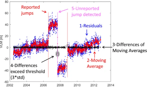
3.1.4 Jump detection
The NGL group invested considerable effort in providing a database that reports jumps in the GPS time-series due to hardware issues (e.g. switching the GPS antenna) and due to geophysical signal (e.g. earthquakes). However, for the purposes of our work (GIA assess-ment) we found that, for a small number of stations, jumps were omitted from the NGL jump database. To detect these unreported jumps, we have designed and implemented an automatic procedure comprising the following steps (Fig.2):
(1) Calculating residual time-series for each station.
(2) Applying a moving average filter to the residual time-series. (3) Computing the differences of the successive moving average values.
(4) Locating groups of jumps with large differences in the moving average values.
(5) Determining the accurate position of the detected jumps.
(1) To calculate the residual time-seriesr, a linear adjustment is applied considering intercepta0, linear trenda1, annual signal with parametersa2anda3, as well as the biasesb=[b1,b2, ...,bJ]
at the reported jump locationsj=1, ...,J
y=a0+a1t+a2sin(2πt)+a3cos(2πt)
+a4sin(4πt)+a5cos(4πt)+Bb+r. (2)
The matrixBcontains the information on the location of the biases. For example, if jumpjoccurs at a time between tk andtk+ 1, the entries in rowBjwill contain zeros prior to the jump occurrence,
that is in columns one tok, and ones after the jump occurrence, that is in columnsk+ 1 to the last columnK(is known as the Heaviside function)
Bj=
0... 0
column˜k
1
column˜k+1
...1
. (3)
The adjusted time-series is subtracted from the original time-series to calculate the residual time-series. (2) An unreported jump will significantly change the average of the residuals within a predefined window. The window length is set to 7 days, which implies that only one unreported jump occurs within 1 week. We consider this reasonable, as the vast majority of jumps are already reported in the NGL database. (3) The differences between the 7-day moving aver-age values provide information on the location of a jump. Thereby, one jump influences seven successively computed average values. (4) To locate these groups of jumps, a threshold of 3σywas selected
for the chosen window length, withσy representing the temporal
variability of the complete available time-seriesy(often called the standard deviation of the time-series). Due to the high noise level within the GPS time-series, a minimum threshold of 3.5 mm was empirically defined. In case that the 3σyvalue is smaller than the
threshold for a time-series, that is that the time-series has a small temporal variability, it is replaced by 2σy, which allowed for a better
detection of unreported jumps. The points of time at which groups of jumps occur provide information on the number of unreported jumps and can be used to separate these groups. (5) The maximum difference of the observed vertical component gives the exact loca-tion of each jump. Finally, the detected jumps are added to the NGL jump database file and this is used for all following computations.
3.1.5 Atmospheric mass loading
It has been shown in previous studies that deformations due to non-tidal atmospheric, oceanic and terrestrial water mass loading have a significant impact on geodetic positioning time-series (e.g. Dach et al.2011; Fritscheet al.2012; van Damet al.2012; Santamar´ıa-G´omez & M´emin2015). The atmospheric mass loading has a spatial wavelength of about 1000 km and effectively adds noise and possi-bly small biases to the vertical linear trends derived from the NGL GPS time-series. Since atmospheric mass loading is well modelled, we use the data provided by the International Mass Loading Ser-vice to compute the loading at the GPS site locations considered in this study (http://massloading.net/). We selected the atmospheric re-analysis product MERRA2 (available from 1980 onwards) and download the product as global 2 ×2maps with a temporal res-olution of 6 hours. The time-series need to be in a reference frame with the origin in the centre of the solid Earth system mass to be consistent with the GPS data set at non-secular periods (Donget al. 2003), which is realized by also downloading gridded global maps representing the degree-1 terms.
3.1.6 Trend and bias estimation
An automatic trend and bias estimation has been implemented, in which the information from the extended jump database (see Section 3.1.4) is used for bias estimation at each jump location. A linear adjustment is performed for each time-series, with intercept a0, linear trenda1, cyclic patterns (represented by a sine and cosine term) with parametersa2anda3for the annual and parametersa4and a5for the semi-annual signal, as well as biasesbfrom the extended jump database (see Section 3.1.4) considered as parameters (similar to, e.g. Roggero2012)
y=a0+a1t+a2sin(2πt)+a3cos(2πt)
+a4sin(4πt)+a5cos(4πt)+Bb+r. (4)
MatrixBis defined in eq. (3). The GPS time-series exhibit tempo-rally correlated (non-Gaussian) noise, which persists in the residual term after ordinary least squares fitting, as identified using the em-pirical autocorrelation function. The ordinary least squares fitting uncertainties for coefficient estimators are derived on the basis that the residual process is independent and identically distributed, and are unreliable if the residual is autocorrelated. Often, power law noise has been estimated to represent the noise level more realisti-cally (e.g. Boset al.2013). Alternatively, Khanet al.(2016) used 30-day averages of the daily vertical solutions to consider tempo-rally correlated noise. The RMS of the 30 daily values to the 30-day average were calculated to represent uncertainties of monthly val-ues and these were used to propagate uncertainties. This approach requires jumps to be removed prior to the estimation of the 30-day average to avoid introducting biases. Therefore, the uncertainty of the jump detection is not included in the final estimation of trend uncertainties.
2168 M. Schumacher et al.
Figure 2.Illustration of the automatic algorithm for jump detection as described in Section 3.1.4. The numbers indicate specific steps described in the text. The vertical lines indicate the position of jumps: red lines show jumps reported in the NGL jump database; and the magenta line shows an unreported jump.
GPS time-series. The final linear trend uncertainties are therefore somewhat larger (but likely more realistic) than those following the approach in Khanet al.(2016).
3.2 Post-processing of GPS uplift rates for GIA purposes
The generic post-processing steps explained in Section 3.1 have to be performed for any GPS time-series analysis and are independent of the application. In this section, we focus on the specific post-processing strategy we have developed to generate a global GPS data set suitable for GIA applications. The strategy accounts for different physical processes, for example hydrological mass load-ing, tectonics and earthquakes (Sections 3.2.1 and 3.2.3), as well as elastic deformation of the Earth crust (Section 3.2.2) and the change of the rotational pole (Section 3.2.4). We also explain how corrections are applied to separate the GIA signal from other sig-nals, and how GPS sites where VLM does not primarily reflect the GIA signal are excluded from our data set. Some of our corrections were not available as time-series, nor were some of the GPS data. Consequently, when applying corrections we used rates throughout and in some cases this could introduce biases due to time-variability of the underlying signal being corrected.
3.2.1 Station selection based on prior information from GIA forward models
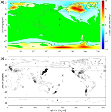
A first selection of NGL GPS sites is performed based on prior information from a set of 13 global GIA forward model solutions to ensure that only stations that primarily represent the GIA signal are considered in the global data set. A mean value of the 13 GIA models and the model spread are calculated for each 1◦×1◦grid cell globally. Then, the globe is divided into seven regions based on the signal strength of GIA and other geophysical signals, for example elastic rebound of the Earth, tectonics or hydrology (Fig.3a): (1) Northern Europe and Asia, (2) North America, (3) mid latitudes, (4) Antarctica, (5) Greenland, (6) Gulf of Alaska, (7) Iceland and (8) Hawaii. The observed uplift rates in some parts of regions (1) and (2) are dominated by the GIA signal (e.g. Scandinavia and Canada), while region (3) is marginally influenced by GIA. In regions (4) and (5) a mixture of GIA signal and elastic response to present-day mass loss is observed, which have to be appropriately accounted
for. In addition, in regions (6) and (7), a mixture of viscous and elastic response of the Earth’s crust, as well as tectonic signals are measured, which are difficult to separate. Regions (4) to (7) are defined based on the Randolph Glacier Inventory (version 6.0) order 1 polygons (RGI Consortium2017).
For each of the regions (1)–(3), the minimum and maximum values of the mean GIA uplift rates, that is the mean of the 13 GIA forward models, are calculated and three times the model spread is either subtracted or added to the values to produce conservative estimates of the range of realistic GIA-related uplift values. We selected three times the empirical standard deviation (i.e. model spread), which corresponds to a 99.7 per cent confidence level, and thus, we ensure a pessimistic estimate of the range limits and do not exclude stations that actually contain a GIA signal. The ranges are, for region (1), between−6 and 16 mm yr−1, region (2) between−10 and 24 mm yr−1and region (3) between−4 and 4 mm yr−1. These limits are used to define which of the GPS sites are selected for the global data set for GIA purposes. GPS sites that exhibit much larger trends are excluded, that is 12.9 per cent of the GPS sites (Fig.3b). It is evident that for some regions a cluster of GPS sites is excluded, for example in Japan (Japan, Izu Ogasawara and Ryuku trench), Malaysia (Java (Sunda) trench), New Zealand (Kermadic trench), Italy (fault line between European and African plates), Chile (Peru-Chile trench) and California (San Andreas fault) which are assumed to be associated with tectonic VLM. In addition, the strong VLM trends in California might be associated with tectonics (Kreemer et al.2010) and the extreme hydrological drought between 2012 and 2016 (Arguset al.2014b; Borsaet al.2014; He & Gautam 2016). In this study, the data for regions (4) and (5), as explained earlier, are replaced by external data sets, and data for regions (6), (7) and (8) are excluded from the data set (see Section 3.2.2 for details).
3.2.2 Elastic correction for ice-covered regions and far field
Figure 3.(a) Mean field of GIA uplift rates from the 13 GIA forward model solutions, and definition of eight regions based on their response to GIA and other geophysical signals: (1) Northern Europe and Asia, (2) North America, (3) mid latitudes, (4) Antarctica, (5) Greenland, (6) Gulf of Alaska, (7) Iceland and (8) Hawaii. (b) Stations that are excluded from the data set for GIA purposes after selecting GPS sites based on prior information from the GIA forward model ensemble. GPS sites in region (1) are marked by squares, in region (2) by crosses and in region (3) by circles.
Greenland, in order to accurately account for the elastic response of the Earth’s crust in these regions. For Antarctica, we use the elastic corrected data set described in Section 2.2 with 65 GPS sites, and for Greenland, the data set described in Section 2.3 with 54 GPS sites. It is clearly visible in Fig.4that neglecting the elastic response would significantly contaminate, and in some areas dominate, the estimated GIA uplift rates. In addition to Antarctica and Greenland, it might be necessary to correct for the elastic rebound of the Earth’s crust also in other glaciated regions, for example the Gulf of Alaska, Iceland Svalbard and Canadian Arctic. Areas underlain with low viscosity mantle, such as the Gulf of Alaska, Iceland and Patagonia, no longer experience substantial GIA signal in response to the last glacial maximum mass loss (Dietrichet al.2010; Satoet al.2011; Auriacet al. 2013). However, the viscous response of the past century since the Little Ice Age is visible in the data (Satoet al. 2011). The GPS data include a mixed signal of this viscous response, of elastic response to present-day mass losses and of tectonics. In Alaska, the latter can constitute a significant part of the signal (Fu & Freymueller2013). Thus, GPS sites in this region are not included in our final global data set (138 GPS sites excluded). Similar issues
can be observed for Iceland, and the corresponding 7 GPS stations are excluded. It is important to note that GRACE detects the viscous response of the Earth’s crust for these regions, which will not be reflected in our global GPS data set, since it is currently not possible to accurately separate the different physical sources observed at these GPS sites in the Gulf of Alaska and Iceland.
2170 M. Schumacher et al.
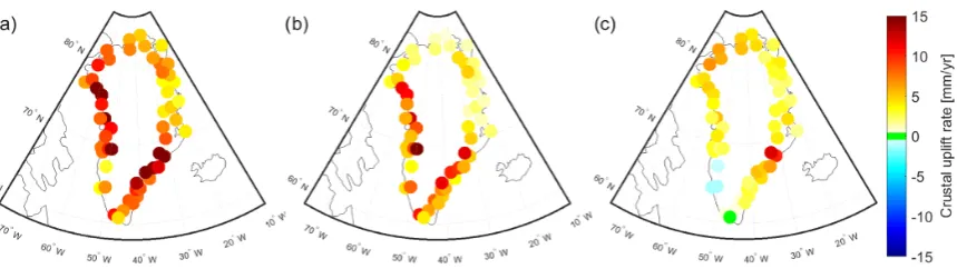
Figure 4.Data set for Greenland: (a) The original GPS uplift rates were corrected due to (b) the elastic response of the solid Earth due to present-day mass losses resulting in the (c) GIA uplift rates.
sitory/uuid:fb667e7a-52f 3-4876-8cab-ae7a2ddaf0db; last access: 2017 October 02) and used in this study to correct for the elastic far field effect of present-day mass losses in regions (1), (2) and (3). It is important to note that this correction includes the effect of changes in the rotational pole (see Section 3.2.4 for details). Based on the grids of Rivaet al.(2017) spanning 2005–2014, we computed uplift rates at the around 4000 considered NGL GPS sites and show them in Fig.5(no data are available for 2015 and it is assumed that the elastic uplift rate does not change during this year). No uncertainties are provided for this correction and are therefore not reflected in the uncertainty estimate of our GPS data set.
3.2.3 Median filter for removal of local and non GIA signals
The non-tidal oceanic and hydrological loading have a similar ef-fect to the atmospheric loading on the GPS time-series but both are less well modelled in general (Santamar´ıa-G´omez & M´emin2015), which means that the loading computations are not as accurate. For example, it would be possible to subtract the hydrological load-ing by removload-ing simulations from global hydrological models with daily time steps as was done by, for example in Simonet al.(2017) for North America. However, numerous studies showed that these models are not in close agreement for many regions worldwide. The representation of long-term trends, in particular, is a common prob-lem among hydrological model simulations (D¨ollet al.2014), which is the component in which we are primarily interested. Therefore, a hydrological mass loading correction would possibly introduce even more uncertainties to our analysis. In addition, a spatial resolution mismatch occurs between GPS observations (point-wise) and mod-els (grid-based, usually provided on 0.5◦or 1◦global grids) which would further increase uncertainties. Thus, no explicit correction is applied for hydrological mass loading in this study but instead we perform a spatial filtering strategy to select stations that are predominantly influenced by the long wavelength GIA signal and to exclude stations that are affected by local to regional hydrology (such as groundwater pumping). This is consistent with Santamar´ıa-G´omez & M´emin (2015), who reported that ‘unless hydrological loading models are improved, there is presently no robust solution to mitigate these uncertainties other than to increase the time-series lengths’.
To ensure that stations influenced by local effects, such as land hydrology and earthquakes (not already filtered out) are removed, we used a low-pass spatial filtering approach. For this, a median filter with a radius of 500 km was applied. We also tested various filters between 250 and 1000 km radius. We found that using a larger radius smoothed the signal too much while, in contrast, using a smaller radius resulted in too few stations available to calculate
the median value. Therefore, 500 km was chosen as a compromise, which roughly represents the correlation lengths of the GIA signal in the forward models. The value at a particular NGL GPS site is assigned the median value within the predefined radius. The dif-ference between the median value and the original value is used as a selection criterion to either keep or remove the station from the global GPS data set. First, stations with an opposite sign of the linear trend before and after the application of the median filter are removed. Subsequently, stations with linear trends that strongly dif-fer before and after the application of the median filter are removed as well. For this, a threshold of three times the uncertainties of the original linear trend was used. This results in 40.1 per cent of the NGL GPS sites being excluded.
3.2.4 Changes in rotational pole
A rapid shift of the Earth’s rotational pole towards the east is ob-served since around 2005, primarily driven by ice sheet melting in Antarctica and Greenland (Chenet al.2013). King & Watson (2014) noted out that the International Earth Rotation Service’s (IERS) elastic pole tide model does not correctly account for this effect. This model is usually used to correct short-term polar mo-tion in geodetic analyses. Hence, the GPS uplift rates determined in this study will be influenced by the deformation resulting from the deviations in polar motion from its longer-term path with a max-imum (minmax-imum) of up to 0.25 mm yr−1 uplift (subsidence) over the U.S. Pacific Coast and South Africa (Europe and south Pacific islands; Fig.6). We used the data set reported in King & Watson (2014) to estimate the effect of polar motion at the considered GPS sites worldwide. The yearly deformations from 1980 to 2015 due to polar motion are used to estimate linear trends over the data period considered at each site, that is 2005–2015 for the NGL sites, 2009– 2013 for the sites in Antarctica, and min./max. 1995/2010 to 2015 depending on the sites in Greenland. These values are subtracted from the GPS uplift rates of the external data sets for Antarctica and Greenland (but not for the NGL sites since the effect is already included in the correction for the far field elastic response described in Section 3.2.2).
3.3 Assessment of GIA forward model solutions
Figure 5.Long wavelength elastic corrections applied for GPS sites within regions (1), (2) and (3). Elastic uplift rate between 2005 and 2014 (no data available for 2015).
Figure 6.Correction for the change in rotational pole in mm yr−1at all considered GPS stations worldwide. The uplift rates due to change in rotational plate are estimated between 2005-2015 for the considered NGL sites, between 2009-2013 for sites in Antarctica, and between 1995/2010-2015 for sites in Greenland (depending on considered data record at each site). The correction is only applied to GPS sites in Antarctica and Greenland, since the effect is already included in the correction for the far field elastic response at the NGL sites.
centre of mass of the solid Earth (CE). The two may be transformed by a translation of the geocentre (e.g. Arguset al.2014a). A con-sistent assessment of the GIA forward model solutions using the global GPS data set is therefore only possible if the origin shift is estimated and removed or a model is applied (Argus & Peltier2010; Kinget al.2012). Thus, we estimated the origin translation between our developed global GPS data set and each of the 13 GIA forward model solutions. The spatial distribution of the GPS sites is far from equal, and this might bias the estimation of the geocentre motion rate. Therefore, we follow the approach described in (Kinget al. 2012, Text S1 of the auxiliary material) using 20◦×10◦windows (the authors proposed 30◦ ×10◦ windows in their paper), i.e. 18 windows in longitudinal and latitudinal direction, and calculated the velocity block median values from the GPS sites contained in each window. These are then converted from the local topocentric systems (setting the velocities of the north and east component to zero) to geocentric cartesian coordinates. The same is repeated for
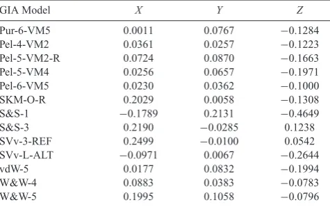
the uplift rates of all provided GIA models but only at the locations of the GPS sites. Linear trends of the CM and CE geocentre in the geocentric coordinate system are derived by averaging over all velocity block median values of the GPS data and the GIA model values, respectively. The difference of the two geocentres is calcu-lated each time, that is CE-CM, and defines the geocentre motion (Table1). It is obvious that the geocentre motion estimate is sen-sitive to the slection of the GIA forward model. The estimate is converted back to north, east and up components in local topocen-tric systems at all GPS sites. Subsequently, the derived corrections of the up component are removed from the GPS uplift rates, that is upC E
G P S=up C M
G P S−upC E−C M, to transform the data set into a
[image:8.595.107.503.278.473.2]2172 M. Schumacher et al.
Table 1. Geocentre motion in terms of cartesian coordinates (in mm yr−1) estimated between the CE origin realized by each individual GIA forward model solution and the CM origin realized by the GPS data set, that is CE-CM.
GIA Model X Y Z
Pur-6-VM5 0.0011 0.0767 −0.1284 Pel-4-VM2 0.0361 0.0257 −0.1223 Pel-5-VM2-R 0.0724 0.0870 −0.1663 Pel-5-VM4 0.0256 0.0657 −0.1971 Pel-6-VM5 0.0230 0.0362 −0.1000 SKM-O-R 0.2029 0.0058 −0.1308 S&S-1 −0.1789 0.2131 −0.4649 S&S-3 0.2190 −0.0285 0.1238 SVv-3-REF 0.2499 −0.0100 0.0542 SVv-L-ALT −0.0971 0.0067 −0.2644 vdW-5 0.0177 0.0832 −0.1994 W&W-4 0.0883 0.0383 −0.0783 W&W-5 0.1995 0.1058 −0.0796
would nonetheless have a very small influence on the GPS uplift rate uncertainties. In summary, the effect of the frame origin transforma-tion on the GPS uplift rates is very small (less than±0.2 mm yr−1 for most GIA models as also found in Kinget al.2012).
4 R E S U L T S A N D D I S C U S S I O N
4.1 The novel GM GPS data set
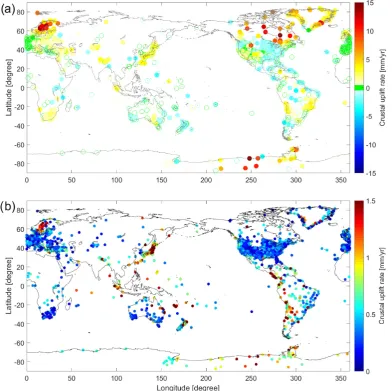
The final post-processed global GM GPS data set is provided in a reference frame with its origin in the centre of mass of the solid Earth (CE). The estimated GIA uplift rates are shown in Fig.8a). It evident that the GIA uplift rates are large in regions that are well known to have been covered by ice during the Last Glacial Maximum approximately 22 000 years ago. In Antarctica, the highest GIA uplift rates occur in the west with rates of up to around 20 mm yr−1, and in Greenland the largest rates of 12 mm yr−1occur close to the Iceland Hot Spot track near Kulusuk at the southeastern coast (Khan et al.2016). Similarly, in Scandinavia and Canada, maximum rates of up to around 14 mm yr−1 are observed. In contrast, at the GPS sites located in lower latitude bands only small trends are present, most of which are statistically insignificant based on a 99 per cent confidence level (shown by hollow circles in Fig.8a). The associated uncertainties of the GIA uplift rates are shown in Fig.8b). The smallest uncertainties of mostly less than 0.5 mm yr−1are estimated for the majority of GPS sites in North America, Europe, many parts of Australia and South Africa. This might be due to the fact that the data records in these regions are usually of very good quality and due to the relatively small trends. Higher uncertainties are obtained for stations along the western coast of South America, the majority of stations in Malaysia and Japan, and for some stations in New Zealand. In these regions, frequently reoccurring earthquakes might influence the quality of the GPS data records, for example many small jumps might be recorded that are not entirely detected and removed from the time-series in the post-processing. In addition, a number of stations in Antarctica, Greenland and Scandinavia show larger uncertainties resulting from the strong GIA uplift rates. In summary, the data set shows a clean GIA signal at all post-processed stations, and is, therefore, suitable to investigate the behaviour of global GIA forward models.
4.2 Comparison to 13 GIA forward model solutions
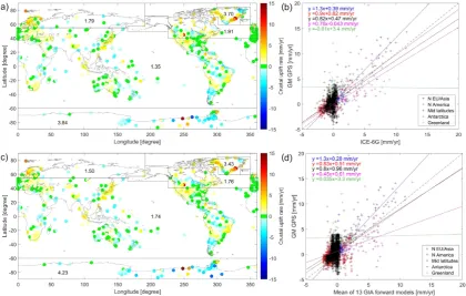
We assess the ICE-6G forward model solution against the GM GPS data set, acknowledging that the latter are not necessarily a per-fect representation of present-day VLM due to GIA. We believe, nonetheless, that they represent the best available data set to test the veracity of GIA forward models. The values in the five regions shown in Fig.9a indicate the spatial RMS difference between the GPS data and the 6G values at all GPS sites (GPS minus ICE-6G). The best agreement is identified for the mid latitudes with an RMS difference of 1.36 mm yr−1, followed by Northern Europe and Asia, as well as North America with 1.71 and 1.94 mm yr−1, respec-tively. The highest discrepancy occurs in Greenland and Antarctica with RMS differences of 3.70 and 3.84 mm yr−1, respectively. This may be due to the use of a relatively low resolution ice mass time-series for GPS elastic correction in the ICE-6G set up (Arguset al. 2014a). In addition, poorly constrained ice loading since the Last Glacial Maximum, as well as uncertainties in lower mantle rheol-ogy, contribute to the differences between GPS data and global GIA forward models.
The differences at the GPS sites show a clear pattern over Scan-dinavia that suggest that the ICE-6G model underestimates GIA uplift rates. In North America, the uplift in the north and the subsi-dence in the centre of the continent towards the south are both too small. At mid latitudes, several spatial patterns are visible. Along the east coast of Australia, New Zealand and Southern America, the model overestimates the GIA uplift rates, which was also re-ported in Kinget al.(2012) for Australia and New Zealand when considering the ICE-5G model but positive differences were found for South America. GPS rates in these regions are negative (Fig.8), so it might be that the ICE-6G model underestimates the magni-tude of the GIA signal or that the signal recorded by the GPS is not related to GIA. In contrast, in Southern Africa, Japan, and the west coast of North America, the model underestimates the uplift rates (also reported in Kinget al.2012,for coast lines and shown here over inland regions also). In addition, it is apparent that in the centre of the South American continent positive differences oc-cur in coastal regions, but negative differences appear inland. The ICE-6G model systematically overestimates the GIA uplift rates in many parts of Antarctica. Poor agreement between the observations and model is found in coastal Greenland. A systematic pattern can be identified with underestimated GIA uplift rates especially along the east and west coast of Greenland. The largest differences occur around the Iceland Hot Spot track near Kulusuk and near Kangerd-lugssuaq (KUAQ; see Khanet al.2016). In summary, GIA rates in Scandinavia, Canada and western part of North America are un-derestimated by the ICE-6G model, as well as along the east and west coast of Greenland, while especially in Antarctica rates are overestimated (see also Fig.9b).
Figure 7.Effect of the difference between the centre of mass of the solid Earth (CE) and the centre of mass of the total Earth’s system (CM), that is CE-CM, on the GPS uplift rates. This correction is subtracted from the estimated GPS uplift rates in the CM frame to obtain the values in the CE frame.
[image:10.595.111.504.279.670.2]2174 M. Schumacher et al.
Figure 9. Assessment of the ICE-6G model and the mean of the 13 GIA forward models using the novel GM GPS data set: (a) Differences between GPS data and the simulated values at 4072 considered GPS sites, that is GPS minus ICE-6G. Numbers indicate the spatial RMS differences averaged over the five regions in mm yr−1. Data in the Gulf of Alaska, Iceland and Hawaii have been excluded. (b) Scatter plot of the GPS data versus the simulated values. Colours in (b) indicate the five regions in (a). The coloured lines indicate the best linear fit for the five regions. (c) Same as (a) but using the mean of the 13 GIA forward models. (d) Same as (b) but using the mean of the GIA models.
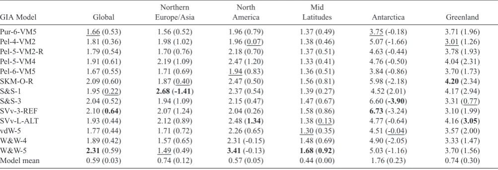
such as, for example, that none of the GIA models take into account ice loss since the end of the little ice age (LIA; 1900). Kjeldsenet al. (2015) showed ice loss since LIA is equivalent to 25 mm of global mean sea level rise, with largest loss in southeast and northwest Greenland, coincident with the largest difference in Figs9a and 9c. We subsequently assessed 13 global GIA forward models against the GM GPS data set, and summarize the results in Table 2. It is evident that no model performs better than any other model in all regions. Globally, the Pur-6-VM5 model shows the best over-all agreement (RMS difference is 1.66 mm yr−1), followed by the ICE-6G model (Pel-6-VM5 in Table2) with a RMS difference of 1.67 mm yr−1. The largest RMS differences are found for Antarc-tica and Greenland for all analysed models where they are on the order of two to three times greater than differences for other con-tinental areas. Since the RMS difference does not provide insights into whether the GIA models over- or underestimate the magnitude of the observed rates, we added the difference of the GPS rates and the GIA model rates averaged over the entire globe and the five regions indicated in Fig.3(Table2). This represents a bias be-tween the observations and the model, and shows whether the GIA model over- or underestimates the (spatial) mean GIA rates for the different regions. The bias should be close to zero if model and ob-servations agree well, at least at the GPS locations. For all regions except Antarctica, the models seem to generally overestimate the mean GIA signal, while in Antarctica 12 out of 13 models under-estimate the mean GIA signal. We also analysed the mean of the 13 GIA models, which statistically should be always closer to the observations (if the number of models is large enough and they are independent, which is only partially the case here due to common ice history models). In terms of RMS differences, this is true for all regions. However, in terms of the bias, this does not hold for
Antarctica, which highlights the large discrepancies between the 13 forward model solutions and the need for additional, for example, observational, information.
5 C O N C L U S I O N S A N D O U T L O O K
Table 2. Assessment of the 13 global GIA forward models and their mean in terms of spatial RMS differences in mm yr−1 and in terms of bias (i.e. the difference of GPS rates and the GIA model rates) averaged over the entire globe and regions 1–5 (Fig.3), that is GPS minus forward model. The best agreement with the novel GM GPS data set is shown by underline, while the worst performance is shown in bold. The model Pel-6-VM5 is identical to the ICE-6G model.
Northern North Mid
GIA Model Global Europe/Asia America Latitudes Antarctica Greenland
Pur-6-VM5 1.66 (0.53) 1.56 (0.52) 1.96 (0.79) 1.37 (0.49) 3.75 (-0.18) 3.71 (1.96) Pel-4-VM2 1.81 (0.36) 1.98 (1.02) 1.96 (0.07) 1.38 (0.46) 5.07 (-1.66) 3.01 (1.26) Pel-5-VM2-R 1.79 (0.54) 1.70 (0.76) 2.18 (0.70) 1.37 (0.51) 4.63 (-0.44) 3.78 (1.93) Pel-5-VM4 1.91 (0.61) 2.19 (1.09) 2.47 (1.20) 1.33 (0.41) 4.76 (-0.50) 4.04 (2.31) Pel-6-VM5 1.67 (0.55) 1.71 (0.69) 1.94 (0.83) 1.36 (0.51) 3.84 (-0.86) 3.70 (1.73) SKM-O-R 2.09 (0.60) 1.87 (0.40) 2.47 (0.50) 1.56 (0.81) 5.98 (-2.18) 4.20(2.34) S&S-1 1.95 (0.22) 2.68(-1.41) 2.37 (0.54) 1.39 (0.27) 4.52 (2.01) 4.17 (2.94) S&S-3 2.04 (0.52) 1.94 (1.09) 2.15 (0.47) 1.47 (0.67) 6.60 (-3.90) 3.31 (0.77) SVv-3-REF 2.10 (0.64) 2.07 (1.24) 2.04 (0.26) 1.58 (0.86) 6.73(-3.24) 3.10 (1.99) SVv-L-ALT 1.93 (0.44) 2.12 (0.89) 2.48 (1.34) 1.38 (0.13) 4.77 (-0.64) 4.16 (3.05) vdW-5 1.77 (0.44) 1.71 (0.72) 2.26 (0.65) 1.30 (0.35) 4.51 (-0.04) 3.57 (2.00) W&W-4 1.89 (0.42) 1.57 (0.65) 2.31 (-0.15) 1.48 (0.69) 4.90 (-2.05) 3.33 (1.47) W&W-5 2.31(0.59) 1.49 (0.49) 3.41(-0.13) 1.68(0.92) 5.03 (-1.16) 3.70 (1.56) Model mean 0.59 (0.03) 0.74 (0.12) 0.57 (0.05) 0.44 (0.00) 1.76 (0.23) 0.74 (0.30)
develop and extend the approach of Mart´ın-Espa˜nolet al.(2016a). The framework will combine global geodetic data on GIA, ice mass and hydrological mass changes, changes in sea level (e.g. from GRACE and altimetry) and prior information from geophysical models to allow new insights about the different contributors to sea level rise on a regional and global scale. The GM GPS data set is available at .
A C K N O W L E D G E M E N T S
M. Schumacher, J. Rougier, Z. Sha, and J.L. Bamber are grateful for the financial support provided by the European Research Council (ERC) under the European Union’s Horizon 2020 research and inno-vation programme under grant agreement no 694188 (GlobalMass project). J.L. Bamber was also supported by a Leverhulme Trust Fellowship (RF-2016-718) and a Royal Society Wolfson Research Merit Award. M.A. King was funded by an Australian Research Council Future Fellowship (project number FT110100207) and sup-ported by the Australian Research Council Special Research Initia-tive for Antarctic Gateway Partnership (Project ID SR140300001). We would like to thank C. Zhang, J.Y. Guo, W. Huang, C.K. Shum and W. van der Wal for providing the ensemble of 13 GIA forward model solutions.
R E F E R E N C E S
Argus, D.F. & Peltier, W.R., 2010. Constraining models of postglacial re-bound using space geodesy: a detailed assessment of model ICE-5G (VM2) and its relatives,Geophys. J. Int.,181,697–723.
Argus, D.F., Peltier, W.R., Drummond, R. & Moore, A.W., 2014a. The Antarctica component of postglacial rebound model ICE-6G C (VM5a) based upon GPS positioning, exposure age dating of ice thicknesses, and relative sea level histories,Geophys. J. Int.,198(1), 537–563.
Argus, D.F., Fu, Y. & Landerer, F.W., 2014b. Seasonal variation in total water storage in California inferred from GPS observations of vertical land motion,Geophys. Res. Lett.,41(6), 1971–1980.
Auriac, A., Spaans, K.H., Sigmundsson, F., Hooper, A., Schmidt, P. & Lund, B., 2013. Iceland rising: solid Earth response to ice retreat inferred from satellite radar interferometry and visocelastic modeling, J. geophys. Res., 118(4), 1331–1344.
Borsa, A.A., Agnew, D.C. & Cayan, D.R., 2014. Ongoing drought-induced uplift in the western United States,Science,345(6204), 1587–1590.
Bos, M.S., Fernandes, R.M.S., Williams, S.D.P. & Bastos, L., 2013. Fast error analysis of continuous GNSS observations with missing data,J. Geod.,87,351–360.
Chen, J.L., Wilson, C.R., Ries, J.C. & Tapley, B.D., 2013. Rapid ice melting drives Earth’s pole to the east,Geophys. Res. Lett.,40,2625–2630. Dach, R., B¨ohm, J., Lutz, S., Steigenberger, P. & Beutler, G., 2011.
Evalu-ation of the impact of atmospheric pressure loading modeling on GNSS data analysis,J. Geod.,85(2), 75–91.
Dietrich, R., Ivins, E.R., Casassa, G., Lange, H., Wendt, J. & Fritsche, M., 2010. Rapid crustal uplift in Patagonia due to enhanced ice lossEarth planet. Sci. Lett.,289(1–2), 22–29.
D¨oll, P., M¨uller Schmied, H., Schuh, C., Portmann, F.T. & Eicker, A., 2014. Global-scale assessment of groundwater depletion and related ground-water abstractions: combining hydrological modeling with information from well observations and GRACE satellites,Water Resour. Res.,50, 56985720.
Dong, D., Yunck, T. & Heflin, M., 2003. Origin of the International Terres-trial Reference Frame,J. geophys. Res.,108(B4), 2200.
Fritsche, M., D¨oll, P. & Dietrich, R., 2012. Global-scale validation of model based load deformation of the Earth’s crust from continental water mass and atmospheric pressure variations using GPS,J. Geodyn.,59–60,133– 142.
Fu, Y. & Freymueller, J.T., 2013. Repeated large slow slip events at the southcentral Alaska subduction zone,Earth planet. Sci. Lett.,375,303– 311.
Guo, J.Y., Huang, W., Shum, C.K. & van der Wal, W., 2012. Comparisons among contemporary glacial isostatic adjustment models,J. Geodyn.,61, 129–137.
Hay, C., Lau, H., Gomez, N., Austermann, J., Powell, E., Mitrovica, J.X., Latychev, K. & Wiens, D., 2017. Sea-level fingerprints in a region of complex Earth structure: the case of WAIS,J. Clim.,30,1881–1892. He, M. & Gautam, M., 2016. Variability and trends in precipitation,
tem-perature and drought indices in the State of California,Hydrology,3(2), 14.
Khan, S.A.et al., 2016. Geodetic measurements reveal similarities between post–Last Glacial Maximum and present-day mass loss from the Green-land ice sheet,Environ. Sci.,2(9), doi:10.1126/sciadv.1600931. King, M.A.et al., 2010. Improved constraints on models of glacial
iso-static adjustment: a review of the contribution of ground-based geodetic observations,Surv. Geophys.,31(5), 465–507.
King, M.A., Keshin, M., Whitehouse, P.L., Thomas, I.D., Milne, G.A. & Riva, R.E.M., 2012. Regional biases in absolute sea level estimates from tide gauge data due to residual unmodeled vertical land movement. Geophys. Res. Lett.,39,L14604, doi:10.1029/2012GL052348. King, M.A. & Watson, C.S., 2014. Geodetic vertical velocities affected by
2176 M. Schumacher et al.
Kjeldsen, K.K.et al., 2015. Spatial and temporal distribution of mass loss from the Greenland Ice Sheet since AD 1900,Nature,528(7582), 396– 400.
Kreemer, C., Blewitt, G. & Hammond, W.C., 2010. Evidence for an active shear zone in southern Nevada linking the Wasatch fault to the Eastern California shear zone,Geology,38(5), 475–478.
Mart´ın-Espa˜nol, A., King, M.A., Zammit-Mangion, A., Andrews, S.B., Moore, P. & Bamber, J.L., 2016a. An assessment of forward and inverse GIA solutions for Antarctica,J. geophys. Res.,121(9), 6947–6965. Mart´ın-Espa˜nol, A.et al., 2016b. Spatial and temporal Antarctic Ice Sheet
mass trends, glacio-isostatic adjustment and surface processes from a joint inversion of satellite altimeter, gravity and GPS data,J. geophys. Res.,121(2), 182–200.
Nield, G.A., Whitehouse, P.L., van der Wal, W., Blank, B., O’Donnell, J.P. & Stuart, G.W., 2018. The impact of lateral variations in lithospheric thickness on glacial isostatic adjustment in West Antarctica,Geophys. J.
Int.,214,811–824.
Peltier, W.R., 2004. Global glacial isostasy and the surface of the ice-age Earth: the ICE-5G (VM2) model and GRACE,Ann. Rev. Earth planet. Sci.,32,111–149.
Peltier, W.R., Argus, D.F. & Drummond, R., 2015. Space geodesy constrains ice-age terminal deglaciation: The global ICE-6G C (VM5a) model,J. geophys. Res.,120,450–487.
Purcell, A., Tregoning, P. & Dehecq, A., 2016. An assessment of the ICE6G C(VM5a) glacial isostatic adjustment model,J. geophys. Res., 121(5), 3939–3950.
Rebischung, P., Griffiths, J., Ray, J., Schmid, R., Collilieux, X. & Garayt, B., 2012. IGS08: the IGS realization of ITRF2008,GPS Solut,16(4), 483–494.
RGI, Consortium, 2017) ,Randolph Glacier Inventory – A Dataset of Global Glacier Outlines: Version 6.0: Technical Report, Global Land Ice
Mea-surements from Space,Colorado, USA. Digital Media.
Riva, R.E.M.et al., 2009. Glacial Isostatic Adjustment over Antarctica from combined ICESat and GRACE satellite data,Earth planet. Sci. Lett., 288(3-4), 516–523.
Riva, R.E.M., Frederikse, T., King, M.A., Marzeion, B. & van den Broeke, M.R., 2017. Brief communication: the global signature of post-1900 land ice wastage on vertical land motion,The Cryosphere,11,1327–1332.
Roggero, M., 2012. Discontinuity detection and removal from data time series, inVII Hotine-Marussi Symposium on Mathematical Geodesy,
In-ternational Association of Geodesy Symposia,Vol.137,eds Sneeuw, N.,
Nov´ak, P., Crespi, M. & Sans`o, F., Springer, Berlin, Heidelberg. Santamar´ıa-G´omez, A. & M´emin, A., 2015. Geodetic secular velocity errors
due to interannual surface loading deformation,Geophys. J. Int.,202(2), 763–767.
Sato, T., Larsen, C.F., Miura, S., Ohta, Y., Fujimoto, H., Sun, W., Motyka, R.J. & Freymueller, J.T., 2011. Reevaluation of the viscoelastic and elastic responses to the past and present-day ice changes in Southeast Alaska, Tectonophysics,511(3–4), 79–88.
Simon, K.M., Riva, R.E.M., Kleinherenbrink, M. & Tangdamrongsuba, N., 2017. A data-driven model for constraint of present-day glacial isostatic adjustment in North America,Earth planet. Sci. Lett.,474,322–333. Spada, G., Ruggieri, G., Sørensen, L.S., Nielsen, K., Melini, D. &
Colleoni, F., 2012. Greenland uplift and regional sea level changes from ICESat observations and GIA modelling,Geophys. J. Int.,189(3), 1457–1474.
van Dam, T., Collilieux, X., Wuite, J., Altamimi, Z. & Ray, J., 2012. Nontidal ocean loading: amplitudes and potential effects in GPS height time series, J. Geod.,86,1043–1057.
van der Wal, W., Whitehouse, P.L. & Schrama, E.J., 2015. Effect of GIA models with 3D mantle viscosity on GRACE mass balance estimates for Antarctica,Earth planet. Sci. Lett.,414,134–143.
Whitehouse, P.L., Bentley, M.J., Milne, G.A., King, M.A. & Thomas, I.D., 2012. A new glacial isostatic adjustment model for Antarctica: calibrated and tested using observations of relative sea-level change and present-day uplift rates,Geophys. J. Int.,190,1464–1482.
W¨oppelmann, G., Letetrel, C., Santamaria, A., Bouin, M.N., Collilieux, X., Altamimi, Z., Williams, S.D.P. & Miguez, B.M., 2009. Rates of sea-level change over the past century in a geocentric reference frame,Geophys. Res. Lett.,36,L12607, doi:10.1029/2009GL038720.
Wu, X.et al., 2010. Simultaneous estimation of global present-day water transport and glacial isostatic adjustment,Nat. Geosci.,3,642–646. Zammit-Mangion, A., Rougier, J., Sch¨on, N., Lindgren, F. & Bamber, J.L.,