An extended orthogonal forward regression algorithm for system identification using entropy

This is a repository copy of An extended orthogonal forward regression algorithm for system identification using entropy.

White Rose Research Online URL for this paper: http://eprints.whiterose.ac.uk/74591/

Monograph:

Guo, L.Z., Billings, S.A. and Zhu, D.Q. (2006) An extended orthogonal forward regression algorithm for system identification using entropy. Research Report. ACSE Research Report no. 931 . Automatic Control and Systems Engineering, University of Sheffield

[email protected] https://eprints.whiterose.ac.uk/ Reuse

Unless indicated otherwise, fulltext items are protected by copyright with all rights reserved. The copyright exception in section 29 of the Copyright, Designs and Patents Act 1988 allows the making of a single copy solely for the purpose of non-commercial research or private study within the limits of fair dealing. The publisher or other rights-holder may allow further reproduction and re-use of this version - refer to the White Rose Research Online record for this item. Where records identify the publisher as the copyright holder, users can verify any specific terms of use on the publisher’s website.

Takedown

If you consider content in White Rose Research Online to be in breach of UK law, please notify us by

An Extended Orthogonal Forward Regression Algorithm for

System Identification Using Entropy

Guo, L. Z., Billings, S. A. and Zhu, D. Q.

Department of Automatic Control and Systems Engineering

University of Sheffield

Sheffield, S1 3JD

UK

An extended orthogonal forward regression

algorithm for system identification using

entropy

Guo, L. Z., Billings, S. A. and Zhu, D. Q.

Department of Automatic Control and Systems Engineering

University of Sheffield

Sheffield S1 3JD, UK

Abstract

In this paper, a fast identification algorithm for nonlinear dynamic stochastic system identification is presented. The algorithm extends the classical Orthogonal Forward Re-gression (OFR) algorithm so that instead of using the Error Reduction Ratio (ERR) for term selection, a new optimality criterion —Shannon’s Entropy Power Reduction Ratio (EPRR) is introduced to deal with both Gaussian and non-Gaussian signals. It is shown that the new algorithm is both fast and reliable and examples are provided to illustrate the effectiveness of the new approach.

1

Introduction

A central part of the conventional OFR algorithm is the Error Reduction Ratio (ERR). The ERR of a term represents the percentage reduction in the total mean square error by including this specific term in the final model. By selecting a term with a maximal ERR value during the implementation of the algorithm, a minimum of the mean square error can be achieved. Therefore, the OFR algorithm is basically minimising a mean square error, the variance of the error in the case of zero-mean variables. This criterion is in line with the traditional approach in stochastic system identification and optimisation problems. The main reason behind this choice of criteria is the assumption that most of the random variables in real-life may be sufficiently described by their second-order statistics, that is their mean and variance. It is well known that Gaussian random variables can be completely defined by the mean value and variance. Therefore, for linear Gaussian systems a criterion based on mean square error would be sufficient to extract all the necessary information from such systems (Papoulis 1991). However, for nonlinear non-Gaussian systems criteria that not only consider the mean value and variance, but also take into account the higher order statistical behaviour of the systems, are much desired. Some recently published papers have addressed this issue (Erdogmus and Principle 2002a, b, Feng, Loparo, and Fang 1997, Ta and DeBrunner 2004, Stoorvogel and van Schuppen 1998). In this paper, differential entropy/ Shannon’s entropy power will be introduced as a new criterion for the nonlinear stochastic system identification problem.

Entropy of a given random variable can be considered as a measure of the average information contained in the probability density function (pdf) of that specific random variable. When the entropy of a random variable is minimised, all moments of the error pdf including the second moments are constrained. It follows therefore that entropy as an optimality criterion extends the concept of mean square error. In particular, it can be shown that the differential entropy is proportional to its variance for Gaussian random variables, and thus minimising entropy is equivalent to the minimisation of the variance/mean square error for Gaussian variables. Using entropy as an optimality criterion has desirable advantages in the dynamic system identification problem because minimising mean square error simply constrains the variance of the identification error between the observed response and the model response, which does not guarantee the capture of all the details of the underlying dynamics. In this paper, an extended OFR algorithm is proposed by accommodating differential entropy/ Shannon’s entropy power as an objective function instead of conventional mean square error. By making use of Shannon’s entropy power inequality, a new quantity —Shannon’s Entropy Power Reduction Ratio (EPRR) —is introduced as an extension of the ERR. It is shown that the model terms can be selected in the same way as the classical OFR algorithm, that is sequentially and independently. This is the main difference between the proposed method and existing methods such as in Erdogmus and Priciple (2002a).

2

Differential entropy and Shannon’s entropy power

in-equality

2.1

Differential entropy and its estimation

Differential entropy of a random variable X with a probability density function fX(·) is defined

as

H(X) =₋

fX(x) logfX(x)dx (1)

Generally, differential entropy can be interpreted as a measure of randomness of X. In the case that X is a Gaussian variable withfX(x) as follows

fX(x) =

1

√

2πσX

exp (₋(x−x¯)

2

2σ2

X

) (2)

where ¯x is the mean value and σ_X2 is the variance. Then it is easy to show that the differential entropy H(X) becomes

H(X) = 1

2log(2πeσ

2

X) (3)

This clearly shows that minimising differential entropy is equivalent to the minimisation of the variance for Gaussian signals.

For a general random variable with finite varianceσ_X2 <_∞, Guo, Shamai, and Verdu (2005) have shown that the differential entropy ofX, regardless of the distribution of X, can be represented as

H(X) = 1

2log(2πeσ

2

X)−

1 2

∞

0

σ_X2

1 +γσ2

X −

E_{(XE_{X_|√γX+N_})2_}dγ (4)

whereE_{·}denotes the expectation,E_{X_|√γX+N_}is the conditional expectation,N _∼N(0,1) is the standard Gaussian which is independent of X. γ is understood as the (gain of the) signal-to-noise ratio of the Gaussian channel whose input is X.

From (4), it can bee observed that the nongaussianness ofX is given by one half of the integral of the difference of the minimum mean square errors achievable by a Gaussian input with variance

σ_X2 and by X, respectively.

variable X, then the Parzen window approximation of its probability density function fX(·) is

ˆ

fX(x) =

1

N

N

i=1

K(x₋xi) (5)

where K(_·) is the kernel function. A Gaussian kernel function is defined as

K(x) = √ 1

2πh2 exp(−

x2

2h2) (6)

where h is the bandwidth of the kernel function. In practice, h can be selected according to Silverman’s rule

h= 1.06σN−1/5 ₍₇₎

in which σ is the standard deviation of the data.

According to the Parzen window estimation ˆfX(x) in (5) of the probability density function and

the definition of differential entropy, an estimation of differential entropy H(X) in (5) can be derived as follows

ˆ

H(X) = ₋

1

N

N

i=1

K(x₋xi)·log(

1

N

N

i=1

K(x₋xi))dx (8)

= ₋ 1

N N j=1 log(1 N N i=1

K(xj −xi))

and if the kernel is Gaussian, this yields

ˆ

H(X) =₋1

N

N

j=1

log(√ 1

2πN h

N

i=1

exp((xj−xi)

2

2h2 )) (9)

2.2

Shannon’s entropy power inequality

Shannon’s power entropy inequality gives a bound on the entropy of the sum of independent random variables as follows

whereX1, X2,· · ·, Xn are n independent random variables. The entropy power is maximum and

equal to the variance when the random variable is Gaussian, and it follows that the essence of Shannon’s entropy power inequality (10) is that the sum of independent variables tends to be “more Gaussian” than individual components. Note that if all of the random variables are Gaussian, (3) yields

2πeσ2 n

i Xi = exp(log(2πeσ 2

n

iXi))≥ n

i

exp(log(2πeσ_X2i)) (11)

Note that because the entropy power of X is exp(2H(X)), from (3), exp(2H(x)) = 2πeσ_X2

for X being Gaussian. This indicates that minimising entropy power is also equivalent to the minimisation of the variance for Gaussian signals.

For given samples x1, x2,· · ·, xN of a random variable X, Shannon’s entropy power ofX can be

approximately calculated according to the estimate ˆH(X) in (8) of differential entropy as follows

exp(2H(X))_≈exp(2 ˆH(X)) = exp(₋21

N

N

j=1

log(1

N

N

i=1

K(xj−xi))) (12)

3

An extended orthogonal forward regression least squares

algorithm

3.1

The classical OFR least-squares algorithm

Let p0, p1,· · ·, pn be random variables and y the output response of a system. Without loss of

generality, all involved variables are assumed to be zero-mean. Assume that there is a subset I

of _{0,1,_{· · ·}, n_}such that a linear relationship

y= i∈I

θipi+ξ (13)

exists, in which ξ is an independent noise variable with zero mean and finite variance. Given a set of observations, the system modelling problem of interest is to determine the subset I and the values of θi. The OFR algorithm for this problem involves three steps

• Orthogonalise the regressors to remove the correlations between these variables;

• Select significant terms using the ERR as a criterion;

Formally, the classical OFR least-squares algorithm can be stated as follows (Billings, Korenberg, and Chen 1988).

Let p0(t), p1(t),· · ·, pn(t) and y(t), t = 1,2,· · ·, N be the series of observations. Denote Y =

(y(1), y(2),_{· · ·}, y(N))T _{and P}

i = (pi(1), pi(2),· · ·, pi(N))T, i = 0,1,· · ·, n, then the following

linear regression model can be formed

Y =P θ+ Ξ (14)

whereP = (P0, P1,· · ·, PN) is the regression matrix,θ = (θ1, θ2,· · ·, θn)T represents the unknown

parameters to be estimated, and Ξ = (ξ(1), ξ(2),_{· · ·}, ξ(N))T _{is some modelling error vector. The}

three steps in the OFR algorithm are

1) ORTHOGONALISATION The orthogonal decomposition P = W A, where A is an (n+ 1)_×(n+ 1) upper triangular matrix with unity diagonal elements, of the regression matrix

P provides an alternative representation of eqn. (14)

Y =P θ+ Ξ =W Aθ+ Ξ =W g+ Ξ (15) where W is an N _×(n+ 1) matrix with orthogonal columns Wi such that WTW =D in

whichDis an (n+1)_×(n+1) diagonal matrix with elementsdi =< Wi, Wi >,i= 0,1,· · ·, n.

Note that < _·,_· > denotes the inner product so that di =< Wi, Wi >= Nt=1wi(t)wi(t),

i= 0,1,_{· · ·}, n.

2) TERM SELECTION The orthogonal least squares solution to g is given by

ˆ

gi =

< Y, Wi >

< Wi, Wi >

= W

T i Y

WT i Wi

, i= 0,1,_{· · ·}, n (16)

The fraction of variance not explained by a regression ofY on W g is

<Ξ,Ξ> < Y, Y > =

< Y ₋W g, Y ₋W g > < Y, Y > =

< Y, Y > ₋< W g, W g >

< Y, Y > (17)

Thus the error reduction ratio (ERR) caused by term i, i= 0,1,_{· · ·}, n is defined as

ERRi =

< Wigi, Wigi >

< Y, Y > (18)

3) PARAMETER ESTIMATION Once the parameters gi, i ∈ I have been estimated using

(16) the parameters θi, i∈I in the regression equation (13) can be calculated as

ˆ

θ =A−1

ˆ

g (19)

From the definition of ERR (18), it can be observed that the OFR is equivalent to maximising the product moment correlation coefficient. In fact, the product moment correlation coefficient

ρi of term i satisfies

ρ2_i = < Y, Wi >

2

< Y, Y >< Wi, Wi >

=

<Y,Wi>2

<Wi,Wi>2 < Wi, Wi >

< Y, Y > =

< Wigi, Wigi >

< Y, Y > =ERRi (20)

3.2

Error reduction ratio (ERR) vs. Shannon’s entropy power

re-duction ratio (EPRR)

Consider the above step 2), that is the Term Selection. This term selection procedure is actually based on the ERR values of each candidate terms. The rationale can be explained as follows (Billings, Chen, and Kronenberg 1989).

For the regression problem (14), the orthogonalised version is that of equation (15). Taking the inner product to (15) gives

< Y, Y >=< W g, Y > +<Ξ, Y > (21)

Substituting Y =W g+ Ξ into the right hand side of (21) yields

< Y, Y >=< W g, W g >+<Ξ,Ξ>=

n

i=0

< Wigi, Wigi >+<Ξ,Ξ> (22)

that is

N

t=1

y2(t) =

n

i=0

N

t=1

g2_iw2_i(t) +

N

t=1

ξ2(t) (23)

assuming thatξ(t) is an independent noise sequence with zero mean and finite variance, and the orthogonality property of columns of the matrix W holds. The maximum mean square error is achieved when no terms are selected to give

Therefore, the reduction in mean square error by including a term Wigi (equivalently Piθi) in

the model will be equal to

< Wigi, Wigi>= N

t=1

g2_iw_i2(t) (25)

It follows that the reduction ratio as a result of including the termPiθiis the percentage reduction

in the total mean square error

ERRi =

< Wigi, Wigi >

< Y, Y > (26)

which is defined as error reduction ratio (ERR) as (18). By selecting a term with a maximal ERR value at a time during the implementation of the algorithm, a minimum of the mean square error can be achieved. This clearly indicates that the above algorithm minimises the mean square error

<Ξ,Ξ>=< Y ₋W g, Y ₋W g >=

N

t=1

(y(t)₋

m

i=0

giwi(t))2 (27)

for any non-negative integer m_≤ n because of the orthogonality property. Note that under the assumption thatξ has zero mean and finite variance, minimising the mean square error<Ξ,Ξ>

is equivalent to minimising the variance ofξ.

Now assume that all involved random variables wi are jointly Gaussian, then they are mutually

independent because the orthogonality of Gaussian variables implies independence. It follows that Shannon’s power entropy inequality holds, that is

exp(2H(y))_≥exp(2H(w1g1)) + exp(2H(w2g2)) +· · ·+ exp(2H(wngn)) + exp(2H(ξ)) (28)

This relationship can be explained as (22). The maximum entropy power of error (equivalently differential entropy of error) is achieved when no terms are selected to give

exp(2H(ξ)) = exp(2H(y)) (29)

variables while the ERR approach is designed to minimise such a variance. Since differential en-tropy has a more general meaning than that of variance for any random variables, it can be used to measure and form a term selection criterion for the general stochastic system identification problem. Following the above discussion, a new criterion, which is called the EPRR (Entropy Power Reduction Ratio), is proposed in this paper as follows.

Notice that Shannon’s entropy power reduction ratio is, as a result of including the termwigi or

piθi, the percentage reduction in the total entropy power

EP RRi =

exp(2H(wigi))

exp(2H(y)) (30)

When wi and y are zero-mean and Gaussian, using (3) and H(wigi) = H(wi) + log|gi|, EPRR

can be expressed as

EP RRi =

exp(2H(wigi))

exp(2H(y)) (31)

= exp(log(2πeσ

2

wi) + log(g 2

i))

exp(log(2πeσ2

y))

= σ

2

wig 2

i

σ2

y

= < Wigi, Wigi >

< Y, Y >

= ERRi

From the definitions of ERR and EPRR, and (4), it can be shown that the EPRR for general random variables can be expressed as follows

EP RRi = ERRi·exp( ∞

0

< Y, Y >₋< Wi, Wi >

(1+< Y, Y >)(1+< Wi, Wi >)

(32)

+(E_{(y₋E_{√γy+Ny})2} −E{(wi−E{wi|√γwi+Nwi}) 2

})dγ)

In practice, the EPRR values can be approximately calculated using (12)

EP RRi ≈gi2· _N

t=1

n

k=1K(y(t)−y(k))

N

k=1K(wi(t)−wi(k))

2 N

3.3

A summary of the proposed extended OFR algorithm

Let Y = (y(1), y(2),_{· · ·}, y(N))T _{and P}

i = (pi(1), pi(2),· · ·, pi(N))T, i = 0,1,· · ·, n be defined as

before, where N is the length of the samples. Then the extended OFR algorithm can now be summarised as follows

Step 1 For i= 0,1,_{· · ·}, n, let W₁(i) =Pi and compute the coefficients g

g(₀i) = < Y, W

(i) 0 >

< W₀(i), W₀(i) > (34)

and their corresponding EPRR using (33)

EP RR(0i) ≈(g (i) 0 )2 ·

_N

t=1

n

k=1K(y(t)−y(k))

N

k=1K(w (i)

0 (t)−w (i) 0 (k))

2 N

(35)

Find the index with a maximal EPRR value h0 = arg[max(EP RR0(i),0 ≤ i ≤ n)] and

select the corresponding term W0 =W(h 0) 0 .

Step l+1 , l _≥1 For 0_≤ i_≤n, i =h0, h1,· · ·, hl−1, calculate the orthogonal projection ofPi on the

linear subspace spanned by W0, W1,· · ·, Wl−1 as follows

W_l(i) =Pi− l−1

j=0

< Pi, Wj >

< Wj, Wj >

Wj (36)

Compute the coefficients g

g(_li) = < Y, W

(i)

l >

< W_l(i), W_l(i) > (37)

and their corresponding EPRR using (33) again

EP RR(_li) _≈(g_l(i))2 _·

_N

t=1

n

k=1K(y(t)−y(k)

N

k=1K(w (i)

l (t)−w

(i)

l (k))

2 N

(38)

Find the index with a maximal EPRR value hl = arg[max(EP RRl(i),0 ≤ i ≤ n), i =

h0, h1,· · ·, hl−1] and select the corresponding term Wl =W

(hl) l .

The procedure is terminated at thenth

s step when

1₋

ns

i=1

EP RRi < ρ (39)

where 0 < ρ < 1 is a prescribed tolerance. This gives a subset model containing ns

Following the determination of the most significant termsW0, W1,· · ·, Wns according to the above

steps, estimates of the parameters θi, i = 0,1,· · ·, ns can be obtained. This can be done using

the following equations

θi = ns

j=i

gjvj (40)

where gi, i= 0,1,· · ·, ns are calculated as follows

gi =

< Y, Wi >

< Wi, Wi >

=

N

t=1y(t)wi(t) N

t=1wi2(t)

, i= 0,1,_{· · ·}, ns (41)

and

vi = 1 (42)

vj = − j−1

k=i

αk,jvk, j =i+ 1,· · ·, n

in which

αk,j =

< Pj, Wk >

< Wk, Wk >

=

N

t=1pj(t)wk(t) N

t=1wk2(t)

, k= 0,1,_{· · ·}, j₋1 (43)

Remark 1 It is worth noting that the algorithm is developed under the assumption that the

involved variables are mutually independent or uncorrelated with a jointly Gaussian distribution. There are some recent results about Shannon’s entropy power inequality for dependent variables (Johnson 2004, Takano 1996). The proposed algorithm projects the regression matrix into an or-thogonal space which implies the involved variables are uncorrelated. Although uncorrelationness does not mean independence, it is, in practice, a good estimation of independence. The examples in this paper show that the extended OFR algorithm works well with this uncorrelationness.

4

Numerical simulations

4.1

Example 1: A linear system with Gaussian and non-Gaussian

noise

−3 −2 −1 0 1 2 0

0.05 0.1 0.15 0.2 0.25 0.3 0.35 0.4

Signal values

Probability density

Figure 1: Example 1: Distribution of a non-Gaussian noise signal with two peaks

Table 1: Example1: The terms and parameters of the final model using the OFR algorithm with Gaussian noise

Terms Estimates ERR

y(t₋1) 1.7749e+000 3.7352e-001

y(t₋2) -1.9534e+000 2.3680e-001

y(t₋3) 1.3874e+000 1.8680e-001

u(t₋1) 9.9466e-001 1.2390e-001

y(t₋4) -4.7615e-001 4.5940e-002

y(t) =a1y(t−1) +a2y(t−2) +a3y(t−3) +a4y(t−4) +a5u(t−1) +e(t) (44)

where a1 = 1.8, a2 = −1.99, a3 = 1.422, a4 = 0.493, and a5 = 1.0. In order to apply the

proposed extended OFR algorithm, system eqn. (44) was simulated where u(t) was a uniformly distributed random signal on the interval [0,1] and two sets of data were collected for the cases where e(t) had a Gaussian (_∼N(0,0.32_{)) and a non-Gaussian probability distribution. Fig. (1)}

shows the probability density function of the applied non-Gaussian noise.

The set of terms in an initial candidate model was set to be _{1, y(t₋1), y(t₋2), y(t₋3), y(t₋

Table 2: Example 1: The terms and parameters of the final model using the extended OFR algorithm with Gaussian noise

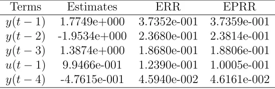
Terms Estimates ERR EPRR

y(t₋1) 1.7749e+000 3.7352e-001 3.7359e-001

y(t₋2) -1.9534e+000 2.3680e-001 2.3814e-001

y(t₋3) 1.3874e+000 1.8680e-001 1.8806e-001

u(t₋1) 9.9466e-001 1.2390e-001 1.0005e-001

y(t₋4) -4.7615e-001 4.5940e-002 4.6161e-002

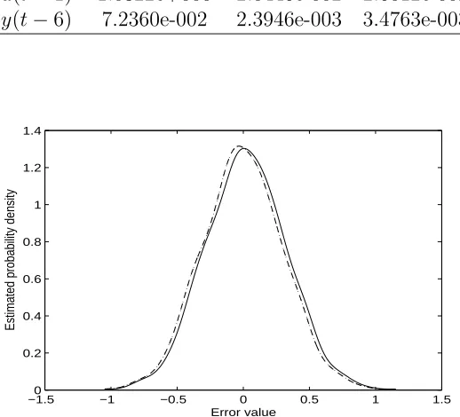
From Tables 1 and 2 it can be observed that the selected significant terms (which are the terms in the original system model) and the parameter estimates are exactly the same (which are very close to the real values) for both algorithms with Gaussian noise, and in this case the ERR values and EPRR values for each selected terms are almost identical. This is because the noise is Gaussian, which verifies the theoretical results, that is that minimising entropy is equivalent to the minimi-sation of variance for Gaussian signals. Furthermore, the estimated higher moments of the errors from both algorithms are coincident (Fig. (3)) : µ3 = 1.4614e−003, µ4 = 2.6130e−002, µ5 =

1.7881e₋003, µ6 = 1.3225e−002, µ7 = 2.1976e−003. Note that the errors from both algorithms

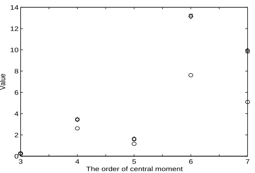
for Gaussian noise have approximated to a Gaussian distribution. This can be observed from Fig. (2) which is the error probability density function estimate calculated using Parzen windowing and Gaussian kernel functions for both algorithms. Therefore, the extended OFR algorithm is equivalent to the original OFR for such Gaussian systems. However, for non-Gaussian noise the results are different. Tables 3 and 4 show that the ERR values and EPRR values are different although all of the correct terms have been selected in the right order by both algorithms. An investigation shows that the higher moments for both algorithms are slightly different as well (Fig. (4)): for the extended OFR algorithm µ3 = 2.4736e −001, µ4 = 3.4510e + 000, µ5 =

1.6009e+ 000, µ6 = 1.3223e+ 001, µ7 = 9.8424e + 000, and for the original OFR algorithm

µ3 = 2.4856e−001, µ4= 3.4393e+000, µ5 = 1.6140e+000, µ6= 1.3129e+001, µ7 = 9.9515e+000.

Table 3: Example1: The terms and parameters of the final model using the OFR algorithm with non-Gaussian noise

Terms Estimates ERR

y(t₋1) 1.9394e+000 5.7413e-001

y(t₋2) -2.1653e+000 1.0629e-001

y(t₋3) 1.5944e+000 1.9971e-001

y(t₋4) -5.1538e-001 2.2979e-002

u(t₋1) 1.0327e+000 2.0446e-002

y(t₋6) 8.6247e-002 2.3946e-003

y(t₋5) -3.2717e-002 2.4375e-005

u(t₋2) -1.3459e-002 2.7265e-006

Table 4: Example 1: The terms and parameters of the final model using the extended OFR algorithm with non-Gaussian noise

Terms Estimates ERR EPRR

y(t₋1) 1.9417e+000 5.7413e-001 5.7422e-001

y(t₋2) -2.1801e+000 1.0629e-001 1.5813e-001

y(t₋3) 1.6272e+000 1.9971e-001 2.6595e-001

y(t₋4) -5.5539e-001 2.2979e-002 3.4981e-002

u(t₋1) 1.0322e+000 2.0446e-002 2.6012e-002

y(t₋6) 7.2360e-002 2.3946e-003 3.4763e-003

−1.50 −1 −0.5 0 0.5 1 1.5

0.2 0.4 0.6 0.8 1 1.2 1.4

Error value

Estimated probability density

3 4 5 6 7 0

0.005 0.01 0.015 0.02 0.025 0.03

The order of central moment

Value

Figure 3: Example 1: Higher central moments of errors of models from conventional OFR (diamond) and extended OFR algorithms (square) for Gaussian noise (the circles denote the higher central moments of the original noise)

3 4 5 6 7

0 2 4 6 8 10 12 14

The order of central moment

Value

−3 −2 −1 0 1 2 3 0

0.05 0.1 0.15 0.2 0.25 0.3 0.35

Error value

Estimated probability density

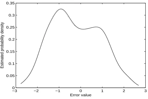
Figure 5: Example 1: Estimated probability distribution of errors of models from original OFR (dotted) and extended OFR algorithms (solid) for non-Gaussian noise

4.2

Prediction of the

Dst

index in Geophysics

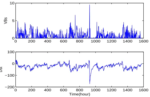
Dstis a geomagnetic index which monitors the world wide magnetic storm level. It is generally constructed by averaging the horizontal component of the geomagnetic field from mid-latitude and equatorial magnetograms from all over the world. Negative Dst values indicate a magnetic storm is in progress, the more negativeDstis the more intense the magnetic storm. The negative deflections in the Dst index are caused by the storm time ring current which flows around the Earth from east to west in the equatorial plane. The ring current results from the differential gradient and curvature drifts of electrons and protons in the near Earth region and its strength is coupled to the solar wind conditions. Only when there is an eastward electric field in the solar wind which corresponds to a southward interplanetary magnetic field (IMF) is there any significant ring current injection resulting in a negative change to the Dst index. In addition to the ring current, other currents such as the current along the magnetopause, a boundary between the terrestrial magnetosphere and the solar wind, also provide some contribution to the evolution of the Dstindex. Due to the importance of the Dstindex, it is highly desirable to be able to predict its values. However, the relationship between the Dst index and the evolution of the ring, magnetopause and magnetotail currents under the influence of the solar wind is extremely complicated. In this study a low dimensional input-output dynamical system model of the magnetosphere will be identified directly from observations using the new approach, in which the input is the product of the solar wind velocity V and the southward component of the solar wind magnetic field Bs and the output is the Dst index. Note that the input was calculated using the plasma velocity and magnetic field measurements from the Wind satellite. The effects of other factors on the system will be neglected in the present study.

0 200 400 600 800 1000 1200 1400 1600 0

5 10

VBs

0 200 400 600 800 1000 1200 1400 1600

−200 −100 0 100

Time(hour)

Dst

Figure 6: Example 2: The input and output data

Table 5: Example2: The terms and parameters of the final model using the extended OFR algorithm

Terms Estimates ERR EPRR

y(t₋1) 1.0569e+000 9.9752e-001 9.9838e-001

y2(t₋2) -1.3591e-001 3.7412e-004 1.3399e-002

y(t₋2)u(t₋1) -4.1862e-001 8.5993e-004 1.3130e-002

y(t₋1)u(t₋2) 1.6460e-001 2.0221e-004 4.9254e-003

y(t₋4)y(t₋7) 7.5858e-002 3.5534e-005 8.2560e-004

u(t₋1) 3.3662e-001 3.0053e-005 4.3869e-004

y(t₋7)u(t₋1) -3.6974e-001 4.9174e-005 9.6667e-004

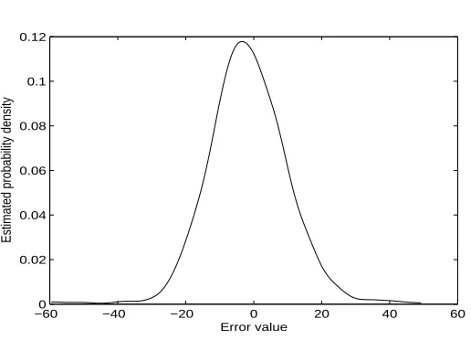
with input lag 3 and output lag 7 and nonlinear degree 2 was used to fit the measured data. The identified final model using the first 500 pairs of data and the extended OFR algorithm is shown in Table 5, which indicates that only 7 out of 66 candidate terms are selected to yields a very simple nonlinear model. A comparison of the test results, that is the output data, the model predicted output and one-step-ahead predicted output, are shown in Fig. (7). The error probability density function estimate calculated using Parzen windowing and Gaussian kernel functions is shown in Fig. (8). The higher moments for the new algorithm are: µ3 =−8.3544e+ 001, µ4 =

0 200 400 600 800 1000 1200 1400 1600 −200

−150 −100 −50 0 50

Time(hour)

Dst(nT)

Figure 7: Example 2: Measurement (solid), model predicted output (dotted) and one-step-ahead predicted output(dashed)

−600 −40 −20 0 20 40 60

0.02 0.04 0.06 0.08 0.1 0.12

Error value

Estimated probability density

From the test results some observations can be made:

1). Both the model predicted and one-step-ahead predicted outputs are good. The model predicted output is not as good as the one-step-ahead predicted output but this is to be expected because model predicted output is a much more severe test than one-step-ahead predictions. However, the model predicted output shows good long-term predictions and gives more confidence in the identified model comparing with the one-step-ahead prediction. Such a model with long-term predictive ability provides a basis for any further analysis and control of the underlying dynamics.

2). Fig. (8) shows that the modelling errors have approximated to a Gaussian distribution, which is different from the estimated pdf from the conventional OFR algorithm.

3). From the final model it can be observed that the main influence of the input (V Bs) on the system current output (Dst) is approximately two hours behind (onlyu(t₋1), u(t₋2) appear in the final model) whilst the influence of the past Dst index on the Dst index is approximately seven hours behind (y(t₋7) appears in the identified model).

4). The discrepancy between the model predicted values and the measured values ofDstmay result from the errors between the real values of the entropy/Shannon entropy power and the estimated values using Parzen windowing and Gaussian kernel functions, high dependence between some candidate model terms, and/or the other factors which actually affect the system dynamics but were not included in the current model.

5

Conclusions

An extended OFR algorithm for the identification of both the model terms or structure and the unknown parameters of non-linear stochastic systems with Gaussian and non-Gaussian noise has been introduced. It has been shown that by using entropy/entropy power as an optimality criterion, the identification ability of the conventional OFR algorithm can be enhanced. The introduction of EPRR in the extended OFR algorithm not only retains the advantages of the OFR algorithm, that is terms can be selected in a fast, simple, and independent way, but also takes into account the higher statistical behaviour of the systems and signals. In this sense the proposed algorithm can be considered as an extension of the conventional OFR algorithm. The method has been tested on both simulated and real data and was shown to perform very well.

6

Acknowledgement

References

[1] Aguirre, L. A. and Billings, S. A., (1995a) Improved structure selection for nonlinear models based on term clustering, Int. J. Contr., Vol. 62, No.3, pp. 569-587.

[2] Aguirre, L. A. and Billings, S. A., (1995b) Retrieving dynamical invariants from chaotic data using narmax models,Int. J. Bifurcation and Chaos, Vol. 5, No. 2, pp. 449-474.

[3] Balikhin, M. A., Zhu, D., and Billings, S. A., (2005) Time domain identification of nonlinear systems: from the measurements to continuous differential equations,The

2005 Joint Assembly Meeting of AGU, SEG, NABS and SPD/AAS, New Orleans,

Louisiana.

[4] Billings, S. A., Chen, S., and Kronenberg, M. J., (1989) Identification of MIMO nonlinear systems using a forward-regression orthogonal estimator, Int. J. Contr., Vol. 49, pp. 2157-2189.

[5] Billings, S. A., Chen, S., and Backhouse, R. J., (1989), The identification of lin-ear and nonlinlin-ear models of a turbocharged automotive diesel engine, Mechanical Systems and Signal Processing, Vol. 3, pp. 123-142.

[6] Billings, S. A., Fadzil, M. B., Sulley, J., and Johnson P. M., (1988), Identification of a nonlinear difference equation model of an industrial diesel generator, Mechanical Systems and Signal Processing, Vol. 2, pp. 59-76.

[7] Billings, S. A., Korenberg, M. J., and Chen, S., (1988) Identification of non-linear output-affine systems using an orthogonal least-squares algorithm, Int. J. Syst. Sci., Vol. 19, pp. 59-76.

[8] Chen, S., Billings, S. A., and Luo, W., (1989) Orthogonal least squares methods and their application to non-linear system identification, International Journal of Control, Vol. 50, No. 5, pp. 1873-1896.

[9] Coca,D. and Billings, S. A., (2001) Identification of coupled map lattice models of complex spatio-temporal pattern, Phys. Lett., A287, pp. 65-73.

[10] Coca, D., Zheng, Y., Mayhew, J., and Billings, S. A. (2000) Nonlinear system identification and analysis of complex dynamical behaviour in reflected light mea-surements of vasomotion, International Journal of Bifurcation and Chaos, Vol. 10, No. 2, pp. 461-476.

[11] Erdogmus, D. and Principe, J. C., (2002a) An error-entropy minimization algo-rithm for supervised training of nonlinear adaptive systems, IEEE Trans. on Signal Processing, Vol. 50, No. 7, pp. 1780-1786.

[13] Feng, X, Loparo, K, and Fang, Y., (1997) Optimal state estimation for stochastic systems: An information theoretic approach, IEEE Trans. Automatic Control, Vol. 42, pp. 771-785.

[14] Guo, D., Shamai, S., and Verdu, S., (2005) Mutual information and minimum mean-square error in Gaussian channels, IEEE Trans. On Information Theory, Vol. 51, No.4, pp. 1261-1282.

[15] Hong, X. and Harris, C. J., (2001) Nonlinear model structure design and construc-tion using orthogonal least squares and d-optimality design, IEEE Transactions on Neural Networks, vol. 13, no. 5, pp. 12451250.

[16] Johnson, O. (2004) A conditional entropy power inequality for dependent variables,

IEEE Trans. Information Theory, Vol. 50, No. 8, pp. 1581-1583.

[17] Liu, J. J., Kung, I. C., and Chao, H. C., (2001) Speed estimate of induction mo-tor using a nonlinear identification technique, Proceedings of the National Science Council, Republic of China. Part A, vol. 25, no. 2, pp. 107-114.

[18] Mao, K. Z., and Billings, S. A., (1997) Algorithms for minimal model structure detection in nonlinear dynamic system identification, Int. J. Control, Vol. 68, pp. 311330.

[19] Mao, K. Z., and Billings, S. A., (1999) Variable selection in nonlinear systems modelling, Mechanical Systems and Signal Processing, Vol. 13, pp. 351366.

[20] Papoulis, A., (1991)Probability, Random Variables, and Stochastic Processes, New York:McGraw-Hill.

[21] Shwartz, S., Zibulevsky, M., and Schechner, Y. Y., (2005) Fast kernel entropy esti-mation and optimization, Signal Processing, Vol. 85, No. 5, pp. 1045-1058.

[22] Stoorvogel, A. A. and van Schuppen, J. H., (1998) Approximation problems with the divergence criterion for Gaussian variables and processes, System & Control Letters, Vol. 35, No. 4, pp. 207-218.

[23] Ta, M. and DeBrunner, V., (2004) Minimum entropy estimation as a near maximum-likelihood method and its application in system identification with non-Gaussian noise, in Proceedings of IEEE International Conference on Acoustics, Speech, and Signal Processing(ICASSP ’04), Vol. 2, pp. 17-21.

[24] Takano, S. (1996) The inequalities of Fisher information and entropy power for dependent variables, inProceedings of 7th Japan-Russia Symposium on Probability Theory and Statistics, Tokyo, pp.460-470.