VIABILITY GRADIENTS IN BIOFILM: A SLIPPERY SLOPE?
1
(Viability Gradients) 2
CK Hope 3
Unit of Plaque Related Diseases, School of Dental Sciences, University of 4
Liverpool. L69 3GN. U.K. 5
6
Abstract 7
Are the fluorescence profiles observed in biofilm an artefact of confocal 8
microscopy and sample topography? A mathematical model has been 9
constructed that replicates these profiles in a homogenous ‘biofilm’. However; 10
direct measurement of metabolic activity in biofilm shows that viability profiles 11
do exist and are therefore structural motifs worthy of study. 12
13
Keywords 14
Cell viability, fluorescence, biofilm, confocal laser scanning microscopy 15
16
Biofilms of bacteria are not homogeneous structures and contain many 17
nonviable cells. These phenomena are due in part to the development of 18
physicochemical gradients within the biofilm, which in turn are manifested as 19
gradients of cell viability. Confocal laser scanning microscopy (CLSM) used in 20
conjunction with fluorescent indicators of cell membrane integrity is a powerful 21
technique for measuring viability gradients within biofilm. However; is it 22
possible that the observations are themselves merely an artefact of confocal 23
microscopy? 24
The confocal scanning microscope was invented in 1955 as a step towards 26
‘the perfect microscope’, one that would be able to examine each point in a 27
specimen and measure the amount of light scattered or absorbed by that 28
individual point (Minsky 1988). It was effectively two microscopes bolted 29
together, one to illuminate a point in the sample with an intense spot of light 30
and another to observe this. The foci of these two microscopes were the 31
same; hence they were termed ‘confocal’. This equipment was developed in 32
the days before lasers, so intense arc illumination sources were used. 33
Although carbon arcs were the brightest available they were unreliable so 34
zirconium arcs, the second brightest, were used instead. Whilst the optical 35
principles of this device worked well, it was extremely difficult to analyse or 36
visualise the data generated. This changed in the 1980’s upon the advent of 37
affordable, reliable computer systems capable of undertaking image analysis 38
and data storage. Modern CLSM uses a focussed spot (or multiple spots or a 39
slit) of laser light to scan across the sample whilst a pinhole aperture blocks 40
aberrant light from areas outside of the focal plane of interest. CLSM has 41
been used for almost two decades to undertake the optical sectioning of 42
microbial biofilms to produce three-dimensional data sets (Lawrence et al. 43
1991). 44
45
Fluorescent dyes (fluorophores) are now a fundamental component of CLSM. 46
Fluorescence is the molecular adsorption of a photon which in turn triggers 47
the emission of another photon of a longer wavelength (due to the Stokes 48
shift); the remaining energy is lost as molecular vibration or shed as heat. Put 49
This phenomenon allows one to illuminate a specific fluorophore with light of 51
one wavelength and selectively collect the resulting emissions using filters to 52
obstruct light of unwanted wavelengths, whilst the confocal optics block light 53
from unwanted focal planes. 54
55
CLSM analysis of biological samples typically uses fluorophores that are 56
associated with specific matrix / biofilm components. In the case of microbial 57
biofilm these fluorophores / targets could included: 58
1. Calcofluor white: Binds to β-linked polysaccharides (i.e. to label 59
extracellular polysaccharide). 60
2. Fluorescent in situ hybridisation (FISH): Detect the presence (or absence) 61
of specific 16s rRNA sequence in multispecies biofilm (i.e. for the 62
identification of microbial species). 63
3. Fluorescent indicators of membrane integrity (i.e. to reveal cell viability). 64
4. Green Fluorescent Protein integrated into the genome (i.e. used as a 65
reporter of gene expression / metabolic activity / biosensor). 66
67
The molecular Probes™ LIVE/DEAD stain system detects nonviable bacteria 68
by a red fluorescent dye (DEAD - propidium iodide) which is membrane 69
impermeant and as such is excluded from entering intact, healthy cells. 70
Viable bacteria are detected by a complimentary, green fluorescent dye (LIVE 71
– SYTO9™) which is membrane permeable and stains all cells. When these 72
dyes intercalate DNA their fluorescence increases significantly, therefore; 73
unbound dyes in the milieu extérieur do not interfere with the detection of the 74
with a damaged membrane), the DEAD stain displaces the LIVE stain from 76
the nucleic acid due to its much higher affinity to intercalate DNA – such a cell 77
will fluoresce red (DEAD). 78
79
CLSM data can be studied by a variety of image analysis techniques to yield 80
numerical data regarding biofilm architecture (Wood et al. 2000), metabolic 81
activity (Macfarlane and Macfarlane 2006), composition (Daims et al. 2006) 82
and commensal interactions (Egland et al. 2004). Our previously published 83
work regarding the spatial distribution of cell vitality in biofilm is based upon 84
depth related trends observed using fluorescent indicators of membrane 85
integrity. These data were gathered by CLSM and derived from plotting the 86
total image fluorescence values against the depth of the optical section into 87
the biofilm (Hope et al. 2002). To facilitate a degree of reproducibility between 88
experiments, a biofilm tower (i.e. a high point) was centred in the confocal 89
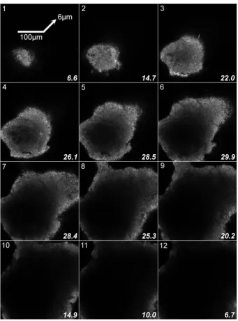
image stack (figure 1). The results typically produced a bell shaped curve of 90
depth-related fluorescence distribution (figure 3). These data were then 91
normalised (i.e. maximum image fluorescence = 1) and used to compare the 92
distribution of viable and nonviable bacteria in biofilm (Hope and Wilson 93
2003a; Hope et al. 2002). Variations of this technique have also been applied 94
by other groups and their findings have been similar to ours (Table 1) (Auschill 95
et al. 2001; Arweiler et al. 2004; Netuschil et al. 1998; Pratten et al. 1998; 96
Zaura-Arite et al. 2001; Hope et al. 2002; Hope and Wilson 2003b; Hope and 97
Wilson 2006; Watson and Robinson 2005; Dalwai et al. 2006). 98
We were initially concerned that the viability profiles revealed by analysing 100
image fluorescence could be an artefact caused by the inter-relationship of 101
biofilm topology and the loss of image contrast which occurs with increasing 102
depth in CLSM imaging. Since the biomass contained within an optical 103
section (generally) increases with depth into the biofilm, this will correspond 104
with an increase in fluorescence due to the presence of more fluorescent 105
material. This effect will be apparent up to a depth of approximately 40 µm, 106
being the point where the absorption of photons emitted by the fluorophore 107
causes image fluorescence to decrease towards zero (Vroom et al. 1999). 108
109
A mathematical model was constructed to demonstrate this perceived 110
phenomenon based upon an idealised hemi-spherical biofilm of radius 80 µm 111
(figure 2). In this model, the amount of fluorescent material within the ‘optical 112
section’ increases with depth into the hemi-sphere. Fluorescence is 113
distributed homogenously within this hemi-spherical model. Quenching of 114
emitted photons is modelled at a linear rate beyond 40 µm depth until total 115
absorbance at the base of the biofilm where no fluorescence is detectable. 116
The resulting ‘fluorescence profile’ through this in silico model (figure 3) is 117
similar to those which have been previously reported in actu (figure 1) and the 118
conformity between these two facets would no doubt be even closer if a more 119
complicated shape and a non-linear co-efficient of adsorption were 120
incorporated into the mathematical model. 121
122
The result of this mathematical model was initially thought to be the reason 123
plaque biofilms were again evident in subgingival plaque – even though 125
individual optical sections presented a nonviable outer layer of bacteria 126
surrounding a viable interior (Hope and Wilson 2006). This contradiction in 127
subgingival plaque biofilm was discussed and it was suggested that if the 128
extent of nonviable bacteria in the outer layers was minimal, then although it 129
might present itself to the observer as nonviable outer layer, it would not affect 130
image analysis of depth related viability / fluorescence profiles. 131
132
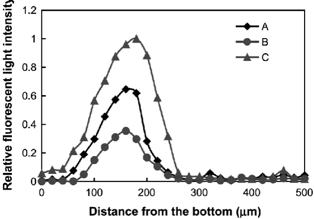
It now seems as though our initial concerns have been allayed after the 133
results published in a recent study (Beyenal et al. 2004). In these 134
experiments, an optical microsensor was used to probe biofilms of 135
Staphylococcus aureus which were engineered to express Yellow Fluorescent 136
Protein. The microsensor measured fluorescence at different points within a 137
biofilm microcolony (figure 4) and reported depth related profiles. They 138
suggested that metabolic activity (vitality) increases with depth in the outer 139
layers of the biofilm before decreasing in the deeper regions. The relative 140
fluorescence profiles produced by the direct microsensor technique, which 141
physically penetrated into the biofilm, were similar to those produced by 142
CLSM. This suggests that viability profiles produced by CLSM are not an 143
artefact of the process by which the images are captured (Table 1). It would 144
be interesting to see if the fluorescence profiles through the S. aureus 145
biofilms, as captured by CLSM, matched those produced by the microsensor. 146
147
Biofilm topography is without doubt an important consideration when using 148
spatial distribution of cell vitality in relation to depth. The reproducibility of this 150
and similar techniques will be improved by taking steps to standardise which 151
structural motifs of biofilm are analysed, along with more advanced 3-152
dimensional analysis (Hope and Wilson 2003b). 153
154
Acknowledgements 155
Thanks to Prof Zbigniew Lewandowski and Dr Haluk Beyenal for permitting 156
the reproduction of the graph in figure 4. Thanks also to Dr John Smalley, 157
University of Liverpool for editorial comments. 158
References 160
161
Arweiler, N.B., Hellwig, E., Sculean, A., Hein, N., and Auschill, T.M. (2004) 162
Individual vitality pattern of in situ dental biofilms at different locations in 163
the oral cavity. Caries Research 38, 442-447. 164
Auschill, T.M., Arweiler, N.B., Netuschil, L., Brecx, M., Reich, E., Sculean, 165
A., and Artweiler, N.B. (2001) Spatial distribution of vital and dead 166
microorganisms in dental biofilms. Archives of Oral Biology 46, 471-476. 167
Beyenal, H., Yakymyshyn, C., Hyungnak, J., Davis, C.C., and 168
Lewandowski, Z. (2004) An optical microsensor to measure fluorescent 169
light intensity in biofilms. Journal of Microbiological Methods 58, 367-374. 170
Daims, H., Lucker, S., and Wagner, M. (2006) daime, a novel image 171
analysis program for microbial ecology and biofilm research. 172
Environmental Microbiology 8, 200-213. 173
Dalwai, F., Spratt, D.A., and Pratten, J. (2006) Modeling shifts in microbial 174
populations associated with health or disease. Applied and Environmental 175
Microbiology 72, 3678-3684. 176
Egland, P.G., Palmer, R.J., Jr., and Kolenbrander, P.E. (2004) Interspecies 177
communication in Streptococcus gordonii-Veillonella atypica biofilms: 178
signaling in flow conditions requires juxtaposition. Proceedings of the 179
National Academy of Sciences of the United States of America 101, 180
16917-16922. 181
Hope, C.K. and Wilson, M. (2003a) Cell vitality within oral biofilms. In Biofilm 182
Communities: Order from Chaos? 269-284. Edited by A. McBain, D. 183
Allison, M. Brading, A. Rickard, J. Verran and J. Walker. Cardiff: BioLine. 184
Hope, C.K., Clements, D., and Wilson, M. (2002) Determining the spatial 185
distribution of viable and nonviable bacteria in hydrated microcosm dental 186
plaques by viability profiling. Journal of Applied Microbiology 93, 448-455. 187
Hope, C.K. and Wilson, M. (2003b) Measuring the thickness of an outer 188
layer of viable bacteria in an oral biofilm by viability mapping. Journal of 189
Microbiological Methods 54, 403-410. 190
Hope, C.K. and Wilson, M. (2006) Biofilm structure and cell vitality in a 191
laboratory model of subgingival plaque. Journal of Microbiological 192
Methods 66, 390-398. 193
Lawrence, J.R., Korber, D.R., Hoyle, B.D., Costerton, J.W., and Caldwell, 194
D.E. (1991) Optical sectioning of microbial biofilms. Journal of Bacteriology 195
173, 6558-6567. 196
Macfarlane, S. and Macfarlane, G.T. (2006) Composition and metabolic 197
activities of bacterial biofilms colonizing food residues in the human gut. 198
Applied and Environmental Microbiology 72, 6204-6211. 199
Minsky, M. (1988) Memoir on Inventing the Confocal Scanning Microscope. 200
Scanning 10, 128-138. 201
Netuschil, L., Reich, E., Unteregger, G., Sculean, A., and Brecx, M. (1998) 202
A pilot study of confocal laser scanning microscopy for the assessment of 203
undisturbed dental plaque vitality and topography. Archives of Oral Biology 204
43, 277-285. 205
Pratten, J., Barnett, P., and Wilson, M. (1998) Composition and 206
susceptibility to chlorhexidine of multispecies biofilms of oral bacteria. 207
Vroom, J.M., De Grauw, K.J., Gerritsen, H.C., Bradshaw, D.J., Marsh, 209
P.D., Watson, G.K., Birmingham, J.J., and Allison, C. (1999) Depth 210
penetration and detection of pH gradients in biofilms by two-photon 211
excitation microscopy. Applied and Environmental Microbiology 65, 3502-212
3511. 213
Watson, P.S. and Robinson, C. (2005) The architecture and microbial 214
composition of natural plaque biofilms. In Biofilms: Persistence and 215
Ubiquity. 273-285. Edited by A. McBain, D. Allison, J. Pratten, D. Spratt, 216
M. Upton, and J. Verran. Cardiff: BioLine. 217
Wood, S.R., Kirkham, J., Marsh, P.D., Shore, R.C., Nattress, B., and 218
Robinson, C. (2000) Architecture of intact natural human plaque biofilms 219
studied by confocal laser scanning microscopy. Journal of Dental 220
Research 79, 21-27. 221
Zaura-Arite, E., van Marle, J., and ten Cate, J.M. (2001) Confocal 222
microscopy study of undisturbed and chlorhexidine-treated dental biofilm. 223
Journal of Dental Research 80, 1436-1440. 224
226
Figure 1 Sequence of twelve optical sections through subgingival oral biofilm 227
stained with SYTO9 (300 x 300 x 72 µm; 6 µm slice separation). The average 228
pixel brightness for individual images is given in the bottom right of each slice. 229
231
Figure 2 Confocal image stack model based upon an idealised hemi-232
spherical biofilm where; R is the radius of the sphere (80 µm), v is the height 233
of the optical section in the image stack and r is the radius of the circle formed 234
by the biofilm (at height v). In this model, the area (a) of a particular optical 235
section can be calculated using the equation, a = π (R2 – v2
) and is equal to 236
the image fluorescence. The fluorescence within the hemi-sphere is 237
distributed homogenously. The absorption of fluorophore photons by the 238
sample is modelled by a linear decrease in fluorescent intensity from 40 µm to 239
80 µm depth (0 to 100% adsorption). 240
241
R r
v
0 - 40 µm No fluorphore absorbtion
40 – 80 µm Linear fluorophore absorbtion (0 – 100%)
Substratum Biofilm
Z
X
Y Optical
242
Figure 3 Fluorescence profile through in actu subgingival plaque biofilm 243
grown in a CDFF (corresponding to figure 1) compared to a mathematical 244
model showing the fluorescence profile through an idealised biofilm in silico 245
(corresponding to figure 2). 246
248
Figure 4 Relative fluorescence intensity profile measured in biofilm of 249
Staphylococcus aureus. Plots A, B and C refer to different sites in a 250
microcolony (Beyenal et al., 2004). 251
Table 1 Studies which comment upon on the spatial distribution of cell vitality 253
in oral biofilm. Asterisks (*) denote the common thread of cell vitality / 254
biomass distribution shown in figure 3. 255
Study Principle Findings
Arweiler 2004
CLSM. Vital staining; measured as percentage vitality in different optical sections.
1. Dead lower layers, live middle / upper layers, less live in outermost layers.*
2. Live lower layers, dead upper layers. 3. Thin disorganised layers.
Auschill 2001
CLSM. Vital staining; measured as percentage vitality in different optical sections.
Dead lower layers, live middle / upper layers, less live in outermost layers.*
Dalwai 2006
CLSM. Vital staining; viable and nonviable fluorescence measured in different optical sections.
Fluorescence distribution low in deep biofilm, higher in the middle layers, decreasing in the outermost layers.*
Hope 2002
CLSM. Vital staining; viable and nonviable compared by normalising fluorescence values in different optical sections.
Dead lower layers, live middle / upper layers, less live in outermost layers.*
Hope 2003
CLSM. Vital staining; analysis of data in 3-dimensions
Dead inner layers, live outer layers.*
Hope 2006
CLSM. Vital staining; viable and nonviable compared by normalising fluorescence values in different optical sections. Subgingival oral biofilm model.
1. Low fluorescence in lower layers, higher in middle / upper layers, lower in outermost layers.* 2. Horizontal sections suggested dead outer layers.
Netuschil 1998
CLSM. Vital staining; measured as percentage vitality.
Dead lower layers, live middle / upper layers, less live in outermost layers.*
Pratten 1998
CLSM vital staining. Dead lower layers, live upper layers.*
Watson 2005
CLSM. Vital staining. Biomass recorded as total image fluorescence.
Low biomass in outer layers, increasing in middle layers, decreasing in deeper layers.*
Zaura-Arite 2001
CLSM. Vital staining. Comparison of percentage vitality at different depths.
No definitive pattern of vitality reported.
Other Related Studies
Study Principle Findings
Beyenal 2004
Direct measurement of Yellow Fluorescent Protein by an optical microsensor in S. aureus. (not oral biofilm, not CLSM)
Low fluorescence (metabolic activity) at biofilm surface, increasing with depth, decreasing in deeper layers.*
Egland 2004
CLSM. Distribution of specifically labelled bacteria (FISH) in a dual-species oral biofilm. (not vital staining)
Fluorescence distribution (biomass) low in deep biofilm, higher in the middle layers, decreasing in the outermost layers.*
Pratten 1998
Transmission electron microscopy. Comparison of cells from different depths in biofilm. (not CLSM)
Higher proportion of ‘ghost’ cells (assumed to be nonviable bacteria) in lower layers.*