Machine Learning in Computer
Vision
by
N. SEBE
University of Amsterdam, The Netherlands
IRA COHEN
ASHUTOSH GARG
and
THOMAS S. HUANG
University of Illinois at Urbana-Champaign, HP Research Labs, U.S.A.
Google Inc., U.S.A.
Published by Springer,
P.O. Box 17, 3300 AA Dordrecht, The Netherlands.
Printed on acid-free paper
All Rights Reserved © 2005 Springer
No part of this work may be reproduced, stored in a retrieval system, or transmitted in any form or by any means, electronic, mechanical, photocopying, microfilming, recording or otherwise, without written permission from the Publisher, with the exception of any material supplied specifically for the purpose of being entered
and executed on a computer system, for exclusive use by the purchaser of the work. Printed in the Netherlands.
To my parents
Nicu
To Merav and Yonatan
Ira
To my parents
Asutosh
To my students: Past, present, and future
Foreword xi
Preface xiii
1. INTRODUCTION 1
1 Research Issues on Learning in Computer Vision 2
2 Overview of the Book 6
3 Contributions 12
2. THEORY:
PROBABILISTIC CLASSIFIERS 15
1 Introduction 15
2 Preliminaries and Notations 18
2.1 Maximum Likelihood Classification 18
2.2 Information Theory 19
2.3 Inequalities 20
3 Bayes Optimal Error and Entropy 20
4 Analysis of Classification Error of Estimated (Mismatched)
Distribution 27
4.1 Hypothesis Testing Framework 28
4.2 Classification Framework 30
5 Density of Distributions 31
5.1 Distributional Density 33
5.2 Relating to Classification Error 37
6 Complex Probabilistic Models and Small Sample Effects 40
vi MACHINE LEARNING IN COMPUTER VISION
3. THEORY:
GENERALIZATION BOUNDS 45
1 Introduction 45
2 Preliminaries 47
3 A Margin Distribution Based Bound 49
3.1 Proving the Margin Distribution Bound 49
4 Analysis 57
4.1 Comparison with Existing Bounds 59
5 Summary 64
4. THEORY:
SEMI-SUPERVISED LEARNING 65
1 Introduction 65
2 Properties of Classification 67
3 Existing Literature 68
4 Semi-supervised Learning Using Maximum Likelihood
Estimation 70
5 Asymptotic Properties of Maximum Likelihood Estimation
with Labeled and Unlabeled Data 73
5.1 Model Is Correct 76
5.2 Model Is Incorrect 77
5.3 Examples: Unlabeled Data Degrading Performance with Discrete and Continuous Variables 80 5.4 Generating Examples: Performance Degradation with
Univariate Distributions 83
5.5 Distribution of Asymptotic Classification Error Bias 86
5.6 Short Summary 88
6 Learning with Finite Data 90
6.1 Experiments with Artificial Data 91
6.2 Can Unlabeled Data Help with Incorrect Models? Bias vs. Variance Effects and the Labeled-unlabeled
Graphs 92
6.3 Detecting When Unlabeled Data Do Not Change the
Estimates 97
6.4 Using Unlabeled Data to Detect Incorrect Modeling
Assumptions 99
5. ALGORITHM:
MAXIMUM LIKELIHOOD MINIMUM ENTROPY HMM 103
1 Previous Work 103
2 Mutual Information, Bayes Optimal Error, Entropy, and
Conditional Probability 105
3 Maximum Mutual Information HMMs 107
3.1 Discrete Maximum Mutual Information HMMs 108 3.2 Continuous Maximum Mutual Information HMMs 110
3.3 Unsupervised Case 111
4 Discussion 111
4.1 Convexity 111
4.2 Convergence 112
4.3 Maximum A-posteriori View of Maximum Mutual
Information HMMs 112
5 Experimental Results 115
5.1 Synthetic Discrete Supervised Data 115
5.2 Speaker Detection 115
5.3 Protein Data 117
5.4 Real-time Emotion Data 117
6 Summary 117
6. ALGORITHM:
MARGIN DISTRIBUTION OPTIMIZATION 119
1 Introduction 119
2 A Margin Distribution Based Bound 120
3 Existing Learning Algorithms 121
4 The Margin Distribution Optimization (MDO) Algorithm 125
4.1 Comparison with SVM and Boosting 126
4.2 Computational Issues 126
5 Experimental Evaluation 127
6 Conclusions 128
7. ALGORITHM:
LEARNING THE STRUCTURE OF BAYESIAN
NETWORK CLASSIFIERS 129
1 Introduction 129
2 Bayesian Network Classifiers 130
2.1 Naive Bayes Classifiers 132
viii MACHINE LEARNING IN COMPUTER VISION
3 Switching between Models: Naive Bayes and TAN Classifiers 138 4 Learning the Structure of Bayesian Network Classifiers:
Existing Approaches 140
4.1 Independence-based Methods 140
4.2 Likelihood and Bayesian Score-based Methods 142 5 Classification Driven Stochastic Structure Search 143 5.1 Stochastic Structure Search Algorithm 143 5.2 Adding VC Bound Factor to the Empirical Error
Measure 145
6 Experiments 146
6.1 Results with Labeled Data 146
6.2 Results with Labeled and Unlabeled Data 147 7 Should Unlabeled Data Be Weighed Differently? 150
8 Active Learning 151
9 Concluding Remarks 153
8. APPLICATION:
OFFICE ACTIVITY RECOGNITION 157
1 Context-Sensitive Systems 157
2 Towards Tractable and Robust Context Sensing 159
3 Layered Hidden Markov Models (LHMMs) 160
3.1 Approaches 161
3.2 Decomposition per Temporal Granularity 162
4 Implementation of SEER 164
4.1 Feature Extraction and Selection in SEER 164
4.2 Architecture of SEER 165
4.3 Learning in SEER 166
4.4 Classification in SEER 166
5 Experiments 166
5.1 Discussion 169
6 Related Representations 170
7 Summary 172
9. APPLICATION:
MULTIMODAL EVENT DETECTION 175
1 Fusion Models: A Review 176
2 A Hierarchical Fusion Model 177
2.1 Working of the Model 178
3 Experimental Setup, Features, and Results 182
4 Summary 183
10. APPLICATION:
FACIAL EXPRESSION RECOGNITION 187
1 Introduction 187
2 Human Emotion Research 189
2.1 Affective Human-computer Interaction 189
2.2 Theories of Emotion 190
2.3 Facial Expression Recognition Studies 192
3 Facial Expression Recognition System 197
3.1 Face Tracking and Feature Extraction 197
3.2 Bayesian Network Classifiers: Learning the
“Structure” of the Facial Features 200
4 Experimental Analysis 201
4.1 Experimental Results with Labeled Data 204
4.1.1 Person-dependent Tests 205
4.1.2 Person-independent Tests 206
4.2 Experiments with Labeled and Unlabeled Data 207
5 Discussion 208
11. APPLICATION:
BAYESIAN NETWORK CLASSIFIERS FOR FACE DETECTION 211
1 Introduction 211
2 Related Work 213
3 Applying Bayesian Network Classifiers to Face Detection 217
4 Experiments 218
5 Discussion 222
References 225
Foreword
It started withimage processing in the sixties. Back then, it took ages to digitize a Landsat image and then process it with a mainframe computer. Pro-cessing was inspired on the achievements of signal proPro-cessing and was still very much oriented towards programming.
In the seventies, image analysis spun off combining image measurement with statistical pattern recognition. Slowly, computational methods detached themselves from the sensor and the goal to become more generally applicable. In the eighties, model-drivencomputer visionoriginated when artificial in-telligence and geometric modelling came together with image analysis compo-nents. The emphasis was on precise analysis with little or no interaction, still very much an art evaluated by visual appeal. The main bottleneck was in the amount of data using an average of 5 to 50 pictures to illustrate the point.
At the beginning of the nineties, vision became available to many with the advent of sufficiently fast PCs. The Internet revealed the interest of the gen-eral public im images, eventually introducing content-based image retrieval. Combining independent (informal) archives, as the web is, urges for interac-tive evaluation of approximate results and hence weak algorithms and their combination in weak classifiers.
In the new century, the last analog bastion was taken. In a few years, sen-sors have become all digital. Archives will soon follow. As a consequence of this change in the basic conditions datasets will overflow. Computer vision will spin off a new branch to be called something like archive-based or se-mantic visionincluding a role for formal knowledge description in an ontology equipped with detectors. An alternative view isexperience-basedorcognitive vision. This is mostly a data-driven view on vision and includes the elementary laws of image formation.
to a broad variety of topics, from a detailed model design evaluated against a few data to abstract rules tuned to a robust application.
From the source to consumption, images are now all digital. Very soon, archives will be overflowing. This is slightly worrying as it will raise the level of expectations about the accessibility of the pictorial content to a level com-patible with what humans can achieve.
There is only one realistic chance to respond. From the trend displayed above, it is best to identify basic laws and then to learn the specifics of the model from a larger dataset. Rather than excluding interaction in the evaluation of the result, it is better to perceive interaction as a valuable source of instant learning for the algorithm.
This book builds on that insight: that the key element in the current rev-olution is the use of machine learning to capture the variations in visual ap-pearance, rather than having the designer of the model accomplish this. As a bonus, models learned from large datasets are likely to be more robust and more realistic than the brittle all-design models.
This book recognizes that machine learning for computer vision is distinc-tively different from plain machine learning. Loads of data, spatial coherence, and the large variety of appearances, make computer vision a special challenge for the machine learning algorithms. Hence, the book does not waste itself on the complete spectrum of machine learning algorithms. Rather, this book is focussed on machine learning for pictures.
It is amazing so early in a new field that a book appears which connects theory to algorithms and through them to convincing applications.
The authors met one another at Urbana-Champaign and then dispersed over the world, apart from Thomas Huang who has been there forever. This book will surely be with us for quite some time to come.
Arnold Smeulders University of Amsterdam The Netherlands
Preface
The goal of computer vision research is to provide computers with human-like perception capabilities so that they can sense the environment, understand the sensed data, take appropriate actions, and learn from this experience in order to enhance future performance. The field has evolved from the applica-tion of classical pattern recogniapplica-tion and image processing methods to advanced techniques in image understanding like model-based and knowledge-based vi-sion.
In recent years, there has been an increased demand for computer vision sys-tems to address “real-world” problems. However, much of our current models and methodologies do not seem to scale out of limited “toy” domains. There-fore, the current state-of-the-art in computer vision needs significant advance-ments to deal with real-world applications, such as navigation, target recogni-tion, manufacturing, photo interpretarecogni-tion, remote sensing, etc. It is widely un-derstood that many of these applications require vision algorithms and systems to work under partial occlusion, possibly under high clutter, low contrast, and changing environmental conditions. This requires that the vision techniques should be robust and flexible to optimize performance in a given scenario.
The field of machine learning is driven by the idea that computer algorithms and systems can improve their own performance with time. Machine learning has evolved from the relatively “knowledge-free” general purpose learning sys-tem, the “perceptron” [Rosenblatt, 1958], and decision-theoretic approaches for learning [Blockeel and De Raedt, 1998], to symbolic learning of high-level knowledge [Michalski et al., 1986], artificial neural networks [Rowley et al., 1998a], and genetic algorithms [DeJong, 1988]. With the recent advances in hardware and software, a variety of practical applications of the machine learn-ing research is emerglearn-ing [Segre, 1992].
and robust vision algorithms, thus improving the performance of practical vi-sion systems. Learning-based vivi-sion systems are expected to provide a higher level of competence and greater generality. Learning may allow us to use the experience gained in creating a vision system for one application domain to a vision system for another domain by developing systems that acquire and maintain knowledge. We claim that learning represents the next challenging frontier for computer vision research.
More specifically, machine learning offers effective methods for computer vision for automating the model/concept acquisition and updating processes, adapting task parameters and representations, and using experience for gener-ating, verifying, and modifying hypotheses. Expanding this list of computer vision problems, we find that some of the applications of machine learning in computer vision are: segmentation and feature extraction; learning rules, relations, features, discriminant functions, and evaluation strategies; learning and refining visual models; indexing and recognition strategies; integration of vision modules and task-level learning; learning shape representation and sur-face reconstruction strategies; self-organizing algorithms for pattern learning; biologically motivated modeling of vision systems that learn; and parameter adaptation, and self-calibration of vision systems. As an eventual goal, ma-chine learning may provide the necessary tools for synthesizing vision algo-rithms starting from adaptation of control parameters of vision algoalgo-rithms and systems.
The goal of this book is to address the use of several important machine learning techniques into computer vision applications. An innovative combi-nation of computer vision and machine learning techniques has the promise of advancing the field of computer vision, which will contribute to better un-derstanding of complex real-world applications. There is another benefit of incorporating a learning paradigm in the computational vision framework. To mature the laboratory-grown vision systems into real-world working systems, it is necessary to evaluate the performance characteristics of these systems us-ing a variety of real, calibrated data. Learnus-ing offers this evaluation tool, since no learning can take place without appropriate evaluation of the results.
Generally, learning requires large amounts of data and fast computational resources for its practical use. However, all learning does not have to be on-line. Some of the learning can be done off-line, e.g., optimizing parameters, features, and sensors during training to improve performance. Depending upon the domain of application, the large number of training samples needed for inductive learning techniques may not be available. Thus, learning techniques should be able to work with varying amounts of a priori knowledge and data.
PREFACE xv
of appropriate representations for the learnable (input) and learned (internal) entities of the system. To succeed in selecting the most appropriate machine learning technique(s) for the given computer vision task, an adequate under-standing of the different machine learning paradigms is necessary.
A learning system has to clearly demonstrate and answer the questions like what is being learned, how it is learned, what data is used to learn, how to rep-resent what has been learned, how well and how efficient is the learning taking place and what are the evaluation criteria for the task at hand. Experimen-tal details are essential for demonstrating the learning behavior of algorithms and systems. These experiments need to include scientific experimental design methodology for training/testing, parametric studies, and measures of perfor-mance improvement with experience. Experiments that exihibit scalability of learning-based vision systems are also very important.
In this book, we address all these important aspects. In each of the chapters, we show how the literature has introduced the techniques into the particular topic area, we present the background theory, discuss comparative experiments made by us, and conclude with comments and recommendations.
Acknowledgments
INTRODUCTION
Computer vision has grown rapidly within the past decade, producing tools that enable the understanding of visual information, especially for scenes with no accompanying structural, administrative, or descriptive text information. The Internet, more specifically the Web, has become a common channel for the transmission of graphical information, thus moving visual information re-trieval rapidly from stand-alone workstations and databases into a networked environment.
Practicality has begun to dictate that the indexing of huge collections of im-ages by hand is a task that is both labor intensive and expensive - in many cases more than can be afforded to provide some method of intellectual ac-cess to digital image collections. In the world of text retrieval, text “speaks for itself” whereas image analysis requires a combination of high-level con-cept creation as well as the processing and interpretation of inherent visual features. In the area of intellectual access to visual information, the interplay between human and machine image indexing methods has begun to influence the development of computer vision systems. Research and application by the image understanding (IU) community suggests that the most fruitful ap-proaches to IU involve analysis and learning of the type of information being sought, the domain in which it will be used, and systematic testing to identify optimal methods.
ad-2 Introduction
vanced applications of image understanding, model-based vision, knowledge-based vision, and systems that exhibit learning capability. The ability to reason and the ability to learn are the two major capabilities associated with these sys-tems. In recent years, theoretical and practical advances are being made in the field of computer vision and pattern recognition by new techniques and pro-cesses of learning, representation, and adaptation. It is probably fair to claim, however, that learning represents the next challenging frontier for computer vision.
1.
Research Issues on Learning in Computer Vision
In recent years, there has been a surge of interest in developing machine learning techniques for computer vision based applications. The interest de-rives from both commercial projects to create working products from com-puter vision techniques and from a general trend in the comcom-puter vision field to incorporate machine learning techniques.
Learning is one of the current frontiers for computer vision research and has been receiving increased attention in recent years. Machine learning technol-ogy has strong potential to contribute to:
the development of flexible and robust vision algorithms that will improve the performance of practical vision systems with a higher level of compe-tence and greater generality, and
the development of architectures that will speed up system development time and provide better performance.
The goal of improving the performance of computer vision systems has brought new challenges to the field of machine learning, for example, learning from structured descriptions, partial information, incremental learning, focus-ing attention or learnfocus-ing regions of interests (ROI), learnfocus-ing with many classes, etc. Solving problems in visual domains will result in the development of new, more robust machine learning algorithms that will be able to work in more realistic settings.
From the standpoint of computer vision systems, machine learning can offer effective methods for automating the acquisition of visual models, adapting task parameters and representation, transforming signals to symbols, building trainable image processing systems, focusing attention on target object, and learning when to apply what algorithm in a vision system.
of learning processes in computer vision systems. Many studies in machine learning assume that a careful trainer provides internal representations of the observed environment, thus paying little attention to the problems of percep-tion. Unfortunately, this assumption leads to the development of brittle systems with noisy, excessively detailed, or quite coarse descriptions of the perceived environment.
Esposito and Malerba [Esposito and Malerba, 2001] listed some of the im-portant research issues that have to be dealt with in order to develop successful applications:
Can we learn the models used by a computer vision system rather than handcrafting them?
In many computer vision applications, handcrafting the visual model of an object is neither easy nor practical. For instance, humans can detect and identify faces in a scene with little or no effort. This skill is quite robust, despite large changes in the visual stimulus. Nevertheless, providing com-puter vision systems with models of facial landmarks or facial expressions is very difficult [Cohen et al., 2003b]. Even when models have been hand-crafted, as in the case of page layout descriptions used by some document image processing systems [Nagy et al., 1992], it has been observed that they limit the use of the system to a specific class of images, which is subject to change in a relatively short time.
How is machine learning used in computer vision systems?
Machine learning algorithms can be applied in at least two different ways in computer vision systems:
– to improve perception of the surrounding environment, that is, to im-prove the transformation of sensed signals into internal representations, and
– to bridge the gap between the internal representations of the environ-ment and the representation of the knowledge needed by the system to perform its task.
4 Introduction
Only recently, the related issues of feature selection and, more generally, data preprocessing have been more systematically investigated in machine learning. Data preprocessing is still considered a step of the knowledge discovery process and is confined to data cleaning, simple data transforma-tions (e.g., summarization), and validation. On the contrary, many studies in computer vision and pattern recognition focused on the problems of fea-ture extraction and selection. Hough transform, FFT, and textural feafea-tures, just to mention some, are all examples of features widely applied in image classification and scene understanding tasks. Their properties have been well investigated and available tools make their use simple and efficient.
How do we represent visual information?
In many computer vision applications, feature vectors are used to represent the perceived environment. However, relational descriptions are deemed to be of crucial importance in high-level vision. Since relations cannot be represented by feature vectors, pattern recognition researchers use graphs to capture the structure of both objects and scenes, while people working in the field of machine learning prefer to use first-order logic formalisms. By mapping one formalism into another, it is possible to find some simi-larities between research done in pattern recognition and machine learning. An example is the spatio-temporal decision tree proposed by Bischof and Caelli [Bischof and Caelli, 2001], which can be related to logical decision trees induced by some general-purpose inductive learning systems [Block-eel and De Raedt, 1998].
What machine learning paradigms and strategies are appropriate to the computer vision domain?
Inductive learning, both supervised and unsupervised, emerges as the most important learning strategy. There are several important paradigms that are being used: conceptual (decision trees, graph-induction), statistical (sup-port vector machines), and neural networks (Kohonen maps and similar auto-organizing systems). Another emerging paradigm, which is described in detail in this book, is the use of probabilistic models in general and prob-abilistic graphical models in particular.
What are the criteria for evaluating the quality of the learning processes in computer vision systems?
How-ever, the comprehensibility of learned models is also deemed an important criterion, especially when domain experts have strong expectations on the properties of visual models or when understanding of system failures is im-portant. Comprehensibility is needed by the expert to easily and reliably verify the inductive assertions and relate them to their own domain knowl-edge. When comprehensibility is an important issue, the conceptual learn-ing paradigm is usually preferred, since it is based on the comprehensibility postulate stated by Michalski [Michalski, 1983]:
The results of computer induction should be symbolic descrip-tions of given entities, semantically and structurally similar to those a human expert might produce observing the same entities. Com-ponents of these descriptions should be comprehensible as single “chunks” of information, directly interpretable in natural language, and should relate quantitative and qualitative concepts in an inte-grated fashion.
When is it useful to adopt several representations of the perceived environ-ment with different levels of abstraction?
In complex real-world applications, multi-representations of the perceived environment prove very useful. For instance, a low resolution document image is suitable for the efficient separation of text from graphics, while a finer resolution is required for the subsequent step of interpreting the sym-bols in a text block (OCR). Analogously, the representation of an aerial view of a cultivated area by means of a vector of textural features can be appropriate to recognize the type of vegetation, but it is too coarse for the recognition of a particular geomorphology. By applying abstraction prin-ciples in computer programming, software engineers have managed to de-velop complex software systems. Similarly, the systematic application of abstraction principles in knowledge representation is the keystone for a long term solution to many problems encountered in computer vision tasks.
How can mutual dependency of visual concepts be dealt with?
6 Introduction
most learning algorithms rely on the independence assumption, according to which the solution to a multiclass or multiple concept learning problem is simply the sum of independent solutions to single class or single concept learning problems.
Obviously, the above list cannot be considered complete. Other equally relevant research issues might be proposed, such as the development of noise-tolerant learning techniques, the effective use of large sets of unlabeled images and the identification of suitable criteria for starting/stopping the learning pro-cess and/or revising acquired visual models.
2.
Overview of the Book
In general, the study of machine learning and computer vision can be di-vided into three broad categories: Theoryleading toAlgorithmsand Applica-tionsbuilt on top of theory and algorithms. In this framework, the applications should form the basis of the theoretical research leading to interesting algo-rithms. As a consequence, the book was divided into three parts. The first part develops the theoretical understanding of the concepts that are being used in developing algorithms in the second part. The third part focuses on the anal-ysis of computer vision and human-computer interaction applications that use the algorithms and the theory presented in the first parts.
results in learning theory falls short of giving any meaningful guarantees for the learned classifiers. This raises a number of interesting questions:
Can we analyze the learning theory for more practical scenarios?
Can the results of such analysis be used to develop better algorithms?
Another set of questions arise from the practical problem of data availabil-ity in computer vision, mainly labeled data. In this respect, there are three main paradigms for learning from training data. The first is known as super-vised learning, in which all the training data are labeled, i.e., a datum contains both the values of the attributes and the labeling of the attributes to one of the classes. The labeling of the training data is usually done by an external mechanism (usually humans) and thus the name supervised. The second is known asunsupervised learningin which each datum contains the values of the attributes but does not contain the label. Unsupervised learning tries to find regularities in the unlabeled training data (such as different clusters under some metric space), infer the class labels and sometimes even the number of classes. The third kind issemi-supervised learningin which some of the data is labeled and some unlabeled. In this book, we are more interested in the latter.
Semi-supervised learning is motivated from the fact that in many computer vision (and other real world) problems, obtaining unlabeled data is relatively easy (e.g., collecting images of faces and non-faces), while labeling is difficult, expensive, and/or labor intensive. Thus, in many problems, it is very desirable to have learning algorithms that are able to incorporate a large number of un-labeled data with a small number of un-labeled data when learning classifiers.
Some of the questions raised in semi-supervised learning of classifiers are:
Is it feasible to use unlabeled data in the learning process?
Is the classification performance of the learned classifier guaranteed to im-prove when adding the unlabeled data to the labeled data?
What is the value of unlabeled data?
The goal of the book is to address all the challenging questions posed so far. We believe that a detailed analysis of the way machine learning theory can be applied through algorithms to real-world applications is very important and extremely relevant to the scientific community.
8 Introduction
a classifier and the conditional entropy of the data. The mismatch between the true underlying model (one that generated the data) and the model used for classification contributes to the second factor of error. In this chapter, we develop bounds on the classification error under the hypothesis testing frame-work when there is a mismatch in the distribution used with respect to the true distribution. Our bounds show that the classification error is closely related to the conditional entropy of the distribution. The additional penalty, because of the mismatched distribution, is a function of the Kullback-Leibler distance be-tween the true and the mismatched distribution. Once these bounds are devel-oped, the next logical step is to see how often the error caused by the mismatch between distributions is large. Our average case analysis for the independence assumptions leads to results that justify the success of the conditional inde-pendence assumption (e.g., in naive Bayes architecture). We show that in most cases, almost all distributions are very close to the distribution assuming condi-tional independence. More formally, we show that the number of distributions for which the additional penalty term is large goes down exponentially fast.
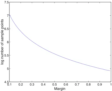
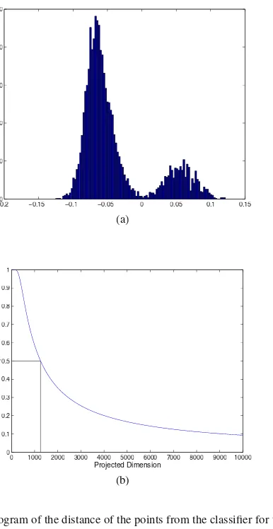
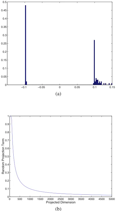
Roth [Roth, 1998] has shown that the probabilistic classifiers can be always mapped to linear classifiers and as such, one can analyze the performance of these under the probably approximately correct (PAC) or Vapnik-Chervonenkis (VC)-dimension framework. This viewpoint is important as it allows one to directly study the classification performance by developing the relations be-tween the performance on the training data and the expected performance on the future unseen data. In Chapter 3, we build on these results of Roth [Roth, 1998]. It turns out that although the existing theory argues that one needs large amounts of data to do the learning, we observe that in practice a good gen-eralization is achieved with a much small number of examples. The existing VC-dimension based bounds (being the worst case bounds) are too loose and we need to make use of properties of the observed data leading to data depen-dent bounds. Our observation, that in practice, classification is achieved with good margin, motivates us to develop bounds based on margin distribution. We develop a classification version of the Random projection theorem [John-son and Lindenstrauss, 1984] and use it to develop data dependent bounds. Our results show that in most problems of practical interest, data actually reside in a low dimensional space. Comparison with existing bounds on real datasets shows that our bounds are tighter than existing bounds and in most cases less than 0.5.
the existing literature, is valid, namely when the assumed probabilistic model matches reality. We also show, both analytically and experimentally, that unla-beled data can be detrimental to the classification performance when the condi-tions are violated. Here we use the term ‘reality’ to mean that there exists some true probability distribution that generates data, the same one for both labeled and unlabeled data. The terms are more rigourously defined in Chapter 4.
The theoretical analysis although interesting in itself gets really attractive if it can be put to use in practical problems. Chapters 5 and 6 build on the results developed in Chapters 2 and 3, respectively. In Chapter 5, we use the results of Chapter 2 to develop a new algorithm for learning HMMs. In Chapter 2, we show that conditional entropy is inversely related to classification performance. Building on this idea, we argue that when HMMs are used for classification, instead of learning parameters by only maximizing the likelihood, one should also attempt to minimize the conditional entropy between the query (hidden) and the observed variables. This leads to a new algorithm for learning HMMs - MMIHMM. Our results on both synthetic and real data demonstrate the su-periority of this new algorithm over the standard ML learning of HMMs.
In Chapter 3, a new, data-dependent, complexity measure for learning – pro-jection profile – is introduced and is used to develop improved generalization bounds. In Chapter 6, we extend this result by developing a new learning algo-rithm for linear classifiers. The complexity measure –projection profile– is a function of themargin distribution(the distribution of the distance of instances from a separating hyperplane). We argue that instead of maximizing the mar-gin, one should attempt to directly minimize this term which actually depends on the margin distribution. Experimental results on some real world problems (face detection and context sensitive spelling correction) and on several UCI data sets show that this new algorithm is superior (in terms of classification performance) over Boosting and SVM.
10 Introduction
structure of a Bayesian network is the graph structure of the network. We show that learning the graph structure of the Bayesian network is key when learn-ing with unlabeled data. Motivated by this observation, we review the existlearn-ing structure learning approaches and point out to their potential disadvantages when learning classifiers. We describe a structure learning algorithm, driven by classification accuracy and provide empirical evidence of the algorithm’s success.
Chapter 8 deals with automatic recognition of high level human behavior. In particular, we focus on the office scenario and attempt to build a system that can decode the human activities (((phone conversation, face-to-face conver-sation, presentation mode, other activity, nobody around,anddistant conver-sation). Although there has been some work in the area of behavioral anal-ysis, this is probably the first system that does the automatic recognition of human activities in real time from low-level sensory inputs. We make use of probabilistic models for this task. Hidden Markov models (HMMs) have been successfully applied for the task of analyzing temporal data (e.g. speech). Al-though very powerful, HMMs are not very successful in capturing the long term relationships and modeling concepts lasting over long periods of time. One can always increase the number of hidden states but then the complexity of decoding and the amount of data required to learn increases many fold. In our work, to solve this problem, we propose the use of layered (a type of hier-archical) HMMs (LHMM), which can be viewed as a special case of Stacked Generalization [Wolpert, 1992]. At each level of the hierarchy, HMMs are used as classifiers to do the inference. The inferential output of these HMMs forms the input to the next level of the hierarchy. As our results show, this new architecture has a number of advantages over the standard HMMs. It allows one to capture events at different level of abstraction and at the same time is capturing long term dependencies which are critical in the modeling of higher level concepts (human activities). Furthermore, this architecture provides ro-bustness to noise and generalizes well to different settings. Comparison with standard HMM shows that this model has superior performance in modeling the behavioral concepts.
the state transition probabilities are modified to explicitly take into account the non-exponential nature of the durations of various events being modeled. Two main features of this model are (a) the ability to account for non-exponential duration and (b) the ability to map discrete state input sequences to decision sequences. The standard algorithms modeling the video-events use HMMs which model the duration of events as an exponentially decaying distribution. However, we argue that the duration is an important characteristic of each event and we demonstrate it by the improved performance over standard HMMs in solving real world problems. The model is tested on the audio-visual event ex-plosion. Using a set of hand-labeled video data, we compare the performance of our model with and without the explicit model for duration. We also com-pare the performance of the proposed model with the traditional HMM and observe an improvement in detection performance.
The algorithms LHMM and DDIOMM presented in Chapters 8 and 9, re-spectively, have their origins in HMM and are motivated by the vast literature on probabilistic models and some psychological studies arguing that human behavior does have a hierarchical structure [Zacks and Tversky, 2001]. How-ever, the problem lies in the fact that we are using these probabilistic models for classification and not purely for inferencing (the performance is measured with respect to the0−1loss function). Although one can use arguments related to Bayes optimality, these arguments fall apart in the case of mismatched dis-tributions (i.e. when the true distribution is different from the used one). This mismatch may arise because of the small number of training samples used for learning, assumptions made to simplify the inference procedure (e.g. a num-ber of conditional independence assumptions are made in Bayesian networks) or may be just because of the lack of information about the true model. Fol-lowing the arguments of Roth [Roth, 1999], one can analyze these algorithms both from the perspective of probabilistic classifiers and from the perspective of statistical learning theory. We apply these algorithms to two distinct but re-lated applications which require machine learning techniques for multimodal information fusion: office activity recognition and multimodal event detection.
12 Introduction
structure learning algorithm yields improved classification results, both in the supervised setting and in the semi-supervised setting.
3.
Contributions
Original contributions presented in this book span the areas of learning ar-chitectures for multimodal human computer interaction, theoretical machine learning, and algorithms in the area of machine learning. In particular, some key issues addressed in this book are:
Theory
Analysis of probabilistic classifiers leading to developing relationship be-tween the Bayes optimal error and the conditional entropy of the distribu-tion.
Bounds on the misclassification error under0−1loss function are devel-oped for probabilistic classifiers under hypothesis testing framework when there is a mismatch between the true distribution and the learned distribu-tion.
Average case analysis of the space of probability distributions. Results ob-tained show that almost all distributions in the space of probability distri-butions are close to the distribution that assumes conditional independence between the features given the class label.
Data dependent bounds are developed for linear classifiers that depend on the margin distribution of the data with respect to the learned classifier.
An extensive discussion of using labeled and unlabeled data for learning probabilistic classifiers. We discuss the types of probabilistic classifiers that are suited for using unlabeled data in learning and we investigate the conditions under which the assertion that unlabeled data are always prof-itable when learning classifiers is valid.
Algorithms
A new learning algorithm MMIHMM (Maximum mutual information HMM) for hidden Markov models is proposed when HMMs are used for classification with states as hidden variables.
A novel learning algorithm - Margin Distribution optimization algorithm is introduced for learning linear classifiers.
Applications
A novel architecture for human activity recognition - Layered HMM - is proposed. This architecture allows one to model activities by combining heterogeneous sources and analyzing activities at different levels of tem-poral abstraction. Empirically, this architecture is observed to be robust to environmental noise and provides good generalization capabilities in dif-ferent settings.
A new architecture based on HMMs is proposed for detecting events in videos. Multimodal events are characterized by the correlation in different media streams and their specific durations. This is captured by the new architecture Duration density Hidden Markov Model proposed in the book.
A Bayesian Networks framework for recognizing facial expressions from video sequences using labeled and unlabeled data is introduced. We also present a real-time facial expression recognition system.
An architecture for frontal face detection from images under various illu-minations is presented. We show that learning Bayesian Networks classi-fiers for detecting faces using our structure learning algorithm yields im-proved classification results both in the supervised setting and in the semi-supervised setting.
This book concentrates on the application domains of human-computer in-teraction, multimedia analysis, and computer vision. However the results and algorithms presented in the book are general and equally applicable to other ar-eas includingspeech recognition, content-based retrieval, bioinformatics,and
Chapter 2
THEORY:
PROBABILISTIC CLASSIFIERS
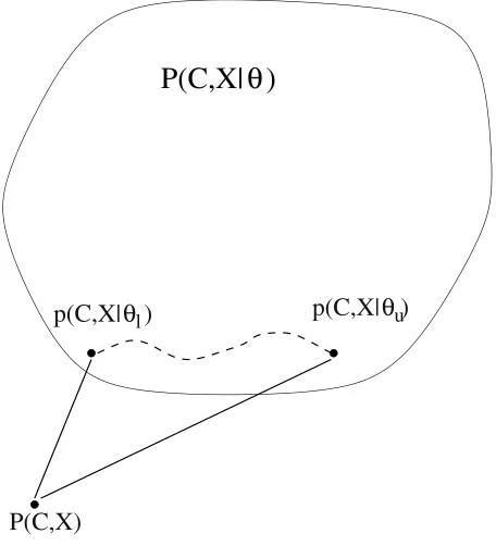
Probabilistic classifiers are developed by assuming generative models which are product distributions over the original attribute space (as in naive Bayes) or more involved spaces (as in general Bayesian networks). While this paradigm has been shown experimentally successful on real world applications, de-spite vastly simplified probabilistic assumptions, the question of why these approaches work is still open.
The goal of this chapter is to give an answer to this question. We show that almost all joint distributions with a given set of marginals (i.e., all distributions that could have given rise to the classifier learned) or, equivalently, almost all data sets that yield this set of marginals, are very close (in terms of distribu-tional distance) to the product distribution on the marginals; the number of these distributions goes down exponentially with their distance from the prod-uct distribution. Consequently, as we show, for almost all joint distributions with this set of marginals, the penalty incurred in using the marginal distri-bution rather than the true one is small. In addition to resolving the puzzle surrounding the success of probabilistic classifiers, our results contribute to understanding the tradeoffs in developing probabilistic classifiers and help in developing better classifiers.
1.
Introduction
The study of probabilistic classification is the study of approximating a joint distribution with a product distribution. Bayes rule is used to estimate the con-ditional probability of a class labely, and then assumptions are made on the model, to decompose this probability into a product of conditional probabili-ties:
P(y|x) =P(y|x1, x2, . . . xn) =
n
i=1
P(xi|x1, . . . xi−1, y)P(y) P(x)
=
n
j=1
P(yj|y)P(y)
P(x), (2.1)
wherex = (x1, . . . , xn)is the observation and theyj =ggj(x1, . . . xi−1, xi),
for some functionggj, are independent given the class labely.
While the use of Bayes rule is harmless, the final decomposition step in-troduces independence assumptions which may not hold in the data. The functions ggj encode the probabilistic assumptions and allow the
representa-tion of any Bayesian network, e.g., a Markov model. The most common model used in classification, however, is the naive Bayes model in which ∀j, g
∀ gj(x1, . . . xi−1, xi) ≡ xi. That is, the original attributes are assumed to
be independent given the class label.
Although the naive Bayes algorithm makes some unrealistic probabilistic assumptions, it has been found to work remarkably well in practice [Elkan, 1997; Domingos and Pazzani, 1997]. Roth [Roth, 1999] gave a partial answer to this unexpected behavior using techniques from learning theory. It is shown that naive Bayes and other probabilistic classifiers are all “Linear Statistical Query” classifiers; thus, PAC type guarantees [Valiant, 1984] can be given on the performance of the classifier on future, previously unseen data, as a func-tion of its performance on the training data, independently of the probabilistic assumptions made when deriving the classifier. However, the key question that underlies the success of probabilistic classifiers is still open. That is, why is it even possible to get good performance on the training data, i.e., to “fit the data”1with a classifier that relies heavily on extremely simplified probabilistic
assumptions on the data?
This chapter resolves this question and develops arguments that could ex-plain the success of probabilistic classifiers and, in particular, that of naive Bayes. The results are developed by doing the combinatoric analysis on the space of all distributions satisfying some properties.
1We assume here a fixed feature space; clearly, by blowing up the feature space it is always possible to fit
Introduction 17
One important point to note is that in this analysis we have made use of the counting arguments to derive most of the results. What that means is that we look at the space of all distributions, where distributions are quantized in some sense (which will be made clear in the respective context), and then we look at these finite number of points (each distribution can be thought of as a point in the distribution space), and try to quantify the properties of this space. This is very different from assuming the uniform prior distribution over the distribution space as this allows our results to be extended to any prior distribution.
This chapter starts by quantifying the optimal Bayes error as a function of the entropy of the data conditioned upon the class label. We develop upper and lower bounds on this term (give the feasible region), and discuss where do most of the distributions lie relative to these bounds. While this gives some idea as to what can be expected in the best case, one would like to quantify what happens in realistic situations, when the probability distribution is not known. Normally in such circumstances one ends up making a number of indepen-dence assumption. Quantifying the penalty incurred due to the indepenindepen-dence assumptions allows us to show its direct relation to the distributional distance between the true (joint) and the product distribution over the marginals used to derive the classifier. This is used to derive the main result of the chapter which, we believe, explains the practical success of product distribution based classi-fiers. Informally, we show thatalmost alljoint distributions with a given set of marginals (that is, all distributions that could have given rise to the classifier learned)2are very close to the product distribution on the marginals - the num-ber of these distributions goes down exponentially with their distance from the product distribution. Consequently, the error incurred when predicting using the product distribution is small foralmost alljoint distributions with the same marginals.
There is no claim in this chapter that distributions governing “practical” problems are sampled according to a uniform distribution over these marginal distributions. Clearly, there are many distributions for which the product dis-tribution based algorithm will not perform well (e.g., see [Roth, 1999]) and in some situations, these could be the interesting distributions. The counting ar-guments developed here suggest, though, that “bad” distributions are relatively rare.
Finally, we show how these insights may allow one to quantify the poten-tial gain achieved by the use of complex probabilistic models thus explaining phenomena observed previously by experimenters.
It is important to note that this analysis ignores small sample effects. We do not attend to learnability issues but rather assume that good estimates of the statistics required by the classifier can be obtained; the chapter concentrates on analyzing the properties of the resulting classifiers.
2.
Preliminaries and Notations
Throughout this chapter we will use capital letter to denote random vari-ables and the same token in lower case (x, y, z) to denote particular instantia-tions of them.P(x|y)will denote the probability of random variableXtaking on valuex, given that the random variableY takes the valuey. Xi denotes theithcomponent of the random vectorX. For a probability distributionP,
P[n](·)denotes the joint probability of observing a sequence ofni.i.d samples distributed according toP.
Throughout the chapter we consider random variables over a discrete do-mainX, of size|X |=N, or overX ×YwhereYis also discrete and typically, |Y| = 2. In these cases, we typically denote byX = {0,1, ..., N −1},Y =
{0,1}.
Definition 2.1 Let X = (X1, X2, ..., Xn) be a random vector over X,
distributed according toQ. Themarginal distributionof theith component of
X, denotedQi, is a distribution overXi, given by
Qi(x) =
xj∈Xj;∀∀ j= i
Q(x1, . . . xi−1, xi, xi+1, . . . xn). (2.2)
Theproduct distributioninduced byQoverX is given by
Qm(x) =
n
i=1
Qi(xi). (2.3)
Note thatQmis identical toQwhen assuming that inQ, the componentsXi
ofXare independent of each other. We sometimes callQm themarginal
dis-tributioninduced byQ.
2.1
Maximum Likelihood Classification
We consider the standard binary classification problem in a probabilistic setting. This model assumes that data elements(x, y) are sampled according to some arbitrary distribution P on X × {0,1}. X is theinstance spaceand
y ∈ {0,1}is called the class label. The goal of the learner is to determine, given a new examplex ∈ X, its most likely corresponding labely(x), which is chosen as follows:
y(x) =argmax
i∈{0,1}
P(y=i|x) =argmax
i∈{0,1}
P(x|y=i)P(y=i)
Preliminaries and Notations 19
Given the distributionP onX × {0,1}, we define the following distributions overX:
P0 P
P =. P(x|y= 0) and PPP1 =. P(x|y= 1). (2.5) With this notation, the Bayesian classifier (in Eqn 2.4) predictsy = 1if and only ifPPP0(x)< PPP1(x).
When X = {0,1}n (or any other discrete product space) we will write
x = (x1, . . . xn) ∈ X, and denote a sample of elements in X by S =
{x1, . . . xm} ⊆ X, with|S| = m. The sample is used to estimate P(x|y),
which is approximated using a conditional independence assumption:
P(x|y) =P(x1, . . . xn|y) =
n
i=1
P(xi|y). (2.6)
Using the conditional independence assumption, the prediction in Eqn 2.4 is done by estimating the product distributions induced byPPP0andPPP1,
Pm
P
P 0 =
n
i=1
P(xi|y= 0) and PPPm1= n
i=1
P(xi|y= 1), (2.7)
and predictingy(x) = 1iff
p(y= 0)PPPm0(x)≤p(y= 1)PPPm1(x). (2.8)
This is typically referred to as the naive Bayes methods of classification [Duda and Hart, 1973].
2.2
Information Theory
Definition 2.2 (Entropy; Kullback-Leibler Distance) Let X
be a random variable overX, distributed according toP.
The entropy ofX(sometimes written as “the entropy ofP”) is given by
H(X) =H(P) =−
x∈X
P(x) logP(x) (2.9)
where the log is to the base 2. Note that the entropy of X can also be in-terpreted as the expected value of logP(1X), which is a function of random variableXdrawn according toP.
The joint entropyH(X, Y)of a pair of discrete random variables(X, Y)
with a joint distributionP(x, y)is defined as
H(X, Y) =−
x∈X
y∈Y
and the conditional entropyH(X|Y)ofXgivenY is defined as
H(X|Y) =−
x∈X
y∈Y
P(x, y) logP(x|y). (2.11)
Let P, Qbe two probability distributions over a discrete domain X. The
relative entropyor theKullback-Leibler distancebetweenP andQis defined as
D(P||Q) =
x∈X
P(x) logP(x)
Q(x) =EEEplog P(X)
Q(X). (2.12)
2.3
Inequalities
1 (Jensen’s Inequality)( [Cover and Thomas, 1991], p. 25) Iff is a convex function andXis a random variable, then
E[f(X)]≥f(E[X]). (2.13)
2 For any probability density functionP over domainX ={1,2, ..., N}we have
H(P) =EP(−logP(X)) =−
N
i=1
pilogpi ≥ −log N
i=1
p2i (2.14)
which follows from Jensen’s inequality using the convexity of−log(x), applied to the random variablep(x), whereX∼p(x).
3 For anyx, k >0, we have
1 + logk−kx≤ −logx (2.15)
which follows fromlog(x) ≤x−1by replacingxbykx. Equality holds whenk= 1/x. Equivalently, replacingxbye−xwe have
1−x≤e−x. (2.16)
For more details please see [Cover and Thomas, 1991].
3.
Bayes Optimal Error and Entropy
In this section, we are interested in the optimal error achievable by a Bayes classifier (Eqn 2.4) on a sample{(x, y)}m1 sampled according to a distribution
Bayes Optimal Error and Entropy 21
class probability case,P(y = 1) =P(y = 0) = 12. The optimal Bayes error is defined by
= 1
2PPP0({x|PPP1(x)> PPP0(x)}) + 1
2PPP1({x|PPP0(x)> PPP1(x)}), (2.17) and the following result relates it to the distance betweenPPP0andPPP1:
Lemma 2.3 ( [Devroye et al., 1996], p. 15) The Bayes optimal error under
the equal class probability assumption is:
= 1
2− 1 4
x
|PPP0(x)−PPP1(x)|. (2.18)
Note thatPPP0(x)andPPP1(x)are “independent” quantities. Theorem 3.2 from [Devroye et al., 1996] also gives the relation between the Bayes optimal error and the entropy of the class label (random variableY ∈ Y) conditioned upon the dataX∈ X:
−log(1−)≤H(Y|X)≡H(P(y|x))≤ −log−(1−) log(1−). (2.19)
However, the availability ofP(y|x)typically depends on first learning a prob-abilistic classifier which might require a number of assumptions. In what fol-lows, we develop results that relate the lowest achievable Bayes error and the conditional entropy of theinput data given the class label, thus allowing an assessment of the optimal performance of the Bayes classifier directly from the given data. Naturally, this relation is much looser than the one given in Eqn 2.19, as has been documented in previous attempts to develop bounds of this sort [Feder and Merhav, 1994]. Let HHHb(p) denote the entropy of the
distribution{p,1−p}:
Hb
H
H (p) =−(1−p) log(1−p)−plogp.
Theorem 2.4 Let X ∈ X denote the feature vector andY ∈ Y, denote
the class label, then under equal class probability assumption, and an optimal Bayes error of, the conditional entropyH(X|Y) of input data conditioned upon the class label is bounded by
1
2HHHb(2)≤H(X|Y)≤HHHb() + log
N
2 . (2.20)
We prove the theorem using the following sequence of lemmas. For simplicity, our analysis assumes that N is an even number. The general case follows similarly. In the following lemmas we consider two probability distributions
P, Q defined over X = {0,1, . . . , N −1}. Let pi = P(x = i) andqi =
wheni < j,pi−qi > pj−qqj(which can always be achieved by renaming the
elements ofX).
Lemma 2.5 Consider two probability distributionsP, Qdefined over X =
{0,1, . . . , N −1}. Let pi = P(x = i) and qi = Q(x = i) and denote
i|pi −qi| = α. Then, the sumH(P) +H(Q) obtains its maximal value
when for some constantsc1, c2, d1, d2 (which depend onα, K, N),P and Q
satisfy:
∀i,0≤i≤M/2 pi=c1, qi =d1 and
∀i, M/2< i≤N pi=c2, qi =d2. (2.21)
Proof. We will first show that,H(P) +H(Q)obtains its maximum value for someK, such that
∀i,0≤i≤K pi =c1, qi=d1 and ∀i, K < i≤N pi =c2, qi =d2,
and will then show that this maximum is achieved forK=M/2. We want to maximize the function
−
i
pilogpi−
i
qilogqi
subject to the constraints
i
|pi−qi|=α,
i
pi = 1,
i
qi = 1.
The Lagrange formulation for the above optimization problem can be written as
λ= −
i
pilogpi−
i
qilogqi
+a
i
|pi−qi| −α
+b
i
pi−1
+c
i
qi−1
,
wherea, b, care Lagrange multipliers. When differentiatingλwith respect to
pi andqi, we obtain that the sum of the two entropies is maximized when, for
some constantsA, B, C,
∀i: 0≤i≤K, pi=Aexp(C), qi =Bexp(−C),
and
∀i:K < i≤N, pi =Aexp(−C), qi=Bexp(C)
Bayes Optimal Error and Entropy 23
Denotep=
K
i=1
piandq =
K
i=1
qi. Then, we have(p−q) + ((1−q)−(1−
p)) =α, giving
0≤i≤K, pi= Kp, qi =pi−2αK
K < i≤N, pi = N1−−pK, qi =pi+2(Nα−K).
These distributions maximizeH(P) +H(Q), which can now be written as
H(P)+++ (H Q) =−plog p
K −(1−p) log
1−p
N −K
−(p−α/2) logp−α/2
K −(1−p+α/2) log
1−p+α/2
N −K .
Differentiating the above expression with respect toK and with respect top, the maximum is achieved whenK =N/2and
p= 1 +α/2
2 , q=
1−α/2
2 . (2.22)
The next lemma is used later to develop the lower bound on the conditional entropy.
Lemma 2.6 Consider two probability distributionsP, Qdefined over X =
{0,1, . . . , N −1}. Let pi = P(x = i) and qi = Q(x = i) and denote
i|pi −qi| = α. The sumH(P) +H(Q) of their entropies is minimized
when all the mass ofQis on single instance i(i.e. qi = 1) with for samei,
pi = 1−α/2and for somej= i,pj =α/2. That is,
P = {0, ..,0, pj =
α
2,0, ...,0, pi= 1−
α
2,0, ..,0} and
Q = {0, ..,0,0,0, ...,0, pi = 1,0, ...,0}.
Proof. Note that for any set of non negative numbersa1, a2, ...,
i
ailogai≤
i
ailog
j
aj ≤
i ai log i ai .
We want to minimize the quantity:
H =−
i
pilogpi−
i
qilogqi,
under the constrainti|pi−qi| = α. As before (Lemma 2.5), assume that
for 0 ≤ i ≤ K, pi ≥ qi and for K < i ≤ N −1, pi ≤ qi, where K ∈
H = −
i
pilogpi−
i
qilogqi
= −
K
i=0
pilogpi− N−1
i=K+1
pilogpi− K
i=0
qilogqi− N−1
i=K+1
qilogqi
≥ −plogp−(1−p) log(1−p)−qlogq−(1−q) log(1−q)(2.23) wherep=Ki=0piandq =
K
i=0qi.
The equality in Eqn 2.22 is achieved if for some0 ≤ j ≤ K,pj =pand
∀i:i= j,0≤i≤K, pi = 0.
In a similar manner, one can write the same equations for(1−p),q, and (1−q). The constraint on the difference of the two distribution, forces that
p−q+ (1−q)−(1−p) =αwhich implies thatp=q+α2. Under this, we can writeHas:
H = − (q+α/2) log(q+α/2)−(1−q−α/2) log(1−q−α/2)
− qlogq−(1−q) log(1−q).
In the above expression,H is a concave function ofq and the minimum (of
H) is achieved when eitherq= 0orq = 1. By symmetryp= α2 andq = 0.
Now we are in a position to prove Theorem 2.4. Lemma 2.5 is used to prove the upper bound and Lemma 2.6 is used to prove the lower bound on the entropy.
Proof. (Theorem 2.4) Assume thatP(y = 0) = P(y = 1) = 12 (equal class probability) and a Bayes optimal error of. For the upper bound onH(X|Y)
we would like to obtainPPP0 andPPP1 that achieve the maximum conditional en-tropy. Since
H(x|y) = P(y = 0)H(PPP0(x)) +P(y = 1)H(PPP1(x))
= 1
2H(PPP0(x)) + 1
2H(PPP1(x)). (2.24) DefiningPPP0 =. P andPPP1 =. Q, the conditional entropy is maximized when the sum ofH(P(x)) +H(Q(x))is maximized. The Bayes optimal error of
constrains the two distribution to satisfyx|PPP0(x)−PPP1(x)|= 2−4=α. Using the result of Lemma 2.5, we obtain the distributions that maximize the conditional entropy as:
P0 P
P =
1 + α
2
N ,
1 + α 2
N , ...,
1− α 2
N ,
1−α 2 N P1 P P =
1−α
2
N ,
1−α 2
N , ...,
1 + α 2
N ,
1 + α 2
N
Bayes Optimal Error and Entropy 25
Note that because of the special form of the above distributions, H(P) = H(Q). The conditional entropyH(X|Y)is given by
H(x|y) = 1
2H(PPP0) + 1
2H(PPP1) =H(PPP0) = −1 +α/2
2 log
1/2 +α/4
N/2 −
1−α/2
2 log
1/2−α/4
N/2
= −1 +α/2
2 log(1/2 +α/4)−
1−α/2
2 log(1/2−α/4) + log
N
2 = −(1−) log(1−)−() log() + logN
2 = HHHb() + log
N
2.
Lemma 2.6 is used to prove the lower bound on the conditional entropy given Bayes optimal error of. The choice of distributions in this case is
P0 P
P = {0,0, ...,1−α
2, ...,0,
α
2,0, ...,0} and
P1 P
P = {0,0, ...,1, ...,0,0,0, ...,0}.
The conditional entropy in this case is given by
H(x|y) = 1
2H(PPP0) + 1 2H(PPP1)
= −(1−α/2) log(1−α/2)−(α/2) log(α/2) + 0
= −(2) log(2)−(1−2) log(1−2)
= HHHb(2).