Abstract: Recently, diatoms, a type of algae microorganism with numerous species, are relatively helpful for water quality determination, and is treated as an important topic in applied biology nowadays. Simultaneously, deep learning (DL) also becomes an important model applied for various image classification problems. This study introduces a new Inception model for diatom image classification. The presented model involves two main stages namely segmentation and classification. Here, a deep learning based Inception model is employed for classification purposes. To further improve the classifier efficiency, edge detection based segmentation model is also applied where the segmented input is provided as an input to the classifier stage. An experimental validation takes place on diverse set of diatom dataset with various preprocessing models. The results pointed out that the presented DL model shows extraordinary classification performance with a classifier accuracy of 99%.
Keywords: Diatom; Segmentation; Classification; Deep Learning.
I. INTRODUCTION
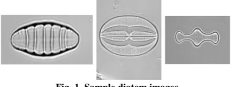
Diatom is a massive and ecologically significant collection of unicellular or colonial organism (algae). It is generally defined by their highly patterned cell wall comprised of hydrated amorphous silica [1]. The cell wall undergoes partition into two halves where every half of the cell wall holds a valve and many girdle bands. One part is somewhat bigger than the other and partly covers it. Jointly, these parts construct a cylinder by two valves at the end. The cross section of the cylinder, and therefore the sketch out of the valve, vary in shape among species and genera to a certain extent. This is collective with the outline of pores and other markings on the valve, offers the details required to classify images [2]. Fig. 1 illustrates three samples of diatom images. Among the different usage of diatoms like water quality monitoring, paleoecology and forensic, microscopic slides should undergo initial scanning for diatoms: when diatoms exists, it is required to be classified. Many classifications should be carried out by the use of classification key and compares the species by the use of slide, photograph or pictures of diatom in books [3]. It is not an insignificant
Revised Manuscript Received on September 03, 2019
A. Victoria Anand Mary,1Research Scholar, Department of Computer Science and Engineering, Annamalai University, India.
G. Prabakaran, 2Assistant Professor, Department of Computer Science and Engineering, Annamalai University, India.
assignment considering that taxonomist computed that it might be 200,000 distinct diatom species, 50% of it is yet to be discovered, and it is very hard to differentiate many of them based on the morphology. In addition, this is extremely tiresome and recurring job, therefore any point of automated process finds more useful. Keeping this view, a new automated diatom classification model is presented which comprises of two traditional portions of image annotation models namely image processing and image classification. The image processing section transforms an image to a collection of numeral features which undergo direct extraction from the pixels of images. The next section performs labeling and grouping of images for classification process. These labels are arranged in a hierarchical way and an image undergoes labeling with many labels which belongs to many groups.
[image:1.595.309.547.557.646.2]Segmentation is a critical process in the investigation and determination of diatoms and other phytoplankton organism due to the fact that it enables the division of the cells from the environment [4]. Image segmentation is normally resolved by the traditional models like thresholding and edge detection, where few variables are generally needed to be predefined earlier. In addition, it is not an automated way which does not need earlier information of the applied models for tuning the segmentation process. Various segmentation models has been implemented, however, the issue lies in the entirely solved, since image segmentation is an important issue with no better option.
Fig. 1. Sample diatom images
The usage of widely used diatom indices always needs an exact level of classification that includes time and expert training. In addition, the determination of morphological microstructures and frustule discrimination from supplementary parts in the image remains challenging. Few diatoms which have treated the similar species for decades have been split into various
species and the introduction of new species is also
An Efficient Automated Deep Learning Model
For Diatom Image Segmentation And
Classification
increasing. The design of automated recognition tools for detection and classification which considers the contour and texture details will be helpful in a broad view of applications for experts as well as non-experts. At the same time, an automated classification of diatom images still remains a big issue. Few methods have been developed for the automated classification of diatoms. But, they mainly depend upon the commonly available features that are constrained and unsuitable for this issue. In addition, the implemented models are useful for a constrained set of species. Therefore, the number of investigated species has been restricted and the performance is bad, reducing the results during a rise in the number of species. In [5], an optimal performance is achieved through the identification of 80 species from the 24K segmented samples with an accuracy of 98.1%. Another massive dataset with 55 species with a minimum number of 1093 samples is presented in [6]. With respect to the usage of deep learning, the limitation is to construct a model which has the ability to differentiate between numerous classes on an average of 700 image samples/class. Many enhanced form of Convolutional Neural Network (CNN) models has been developed [7, 8].
This study introduces a new Inception model for automated diatom image classification model. The presented model involves two main stages namely segmentation and classification. Here, a deep learning based Inception model is employed for classification purposes. To further improve the
classifier efficiency, canny edge detection based segmentation model is also applied where the segmented input is provided as an input to the classifier stage. An experimental validation takes place on diverse set of diatom dataset with various preprocessing models. The results pointed out that the presented DL model shows extraordinary classification performance with a classifier accuracy of 99%. The upcoming portions are arranged as follows. Section 2 discusses the projected DL model for diatom classification and Section 3 evaluates the presented model. Finally, Section 4 draws the conclusion.
II. PROPOSED MODEL
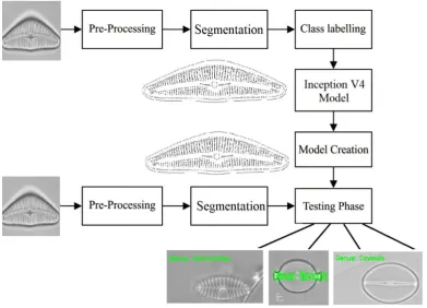
[image:2.595.100.492.423.705.2]The working principle of the presented model is shown in Fig. 2. As illustrated, the input image undergoes preprocessing stages at the beginning. Then, the pre-processed images are segmented by the use of canny edge detection method [9]. Next, class labeling and training takes place utilizing Inception V4 model. In addition, the outcome of the Inception V4 produces a model [10] which has the ability to test the input raw images. Once the model has been generated, it is available for the testing of the new images. On providing the test image as input, the preprocessing and segmentation process will takes place. Then, the segmented image will be tested to produce the outcome. The constructed model will test the provided input and generates the corresponding classifier outputs.
A. Canny Edge Detection Technique for Image Segmentation
Edge detection forms the basic process of segmenting the images. It converts the raw images to the edge images which gets the advantageous from the variations of grey tones in the image. During the image processing tasks, edge detection considers the localization of essential differences present in a grayscale image and the recognition of the physical and geometrical properties of objects of the scene. It is a fundamental process detects and outlines of an object and borders between the objects and environment in the image. Edge detection is the popular way of identifying important discontinuity among intensity values. Edges are local variations in the image intensity. Edges classically appear at the border of the two portions. The important characteristics can be filtered from the image edges. Since different models are applied for edge detection, the canny edge detection method is an optimal model due to the fact it comprises few modifiable variables that can influence the speed and efficiency of the technique.
• Gaussian Filter Size: The performance of the identification of small and sharp lines is openly influenced through the smoothing filter employed in initial phase. A large filter leads to blurred image from the value of the provided pixel over massive portions of the image.
[image:3.595.52.289.474.610.2]• The usage of two thresholds with hysteresis enables more flexible nature over a single-threshold. A higher threshold value leads to loss of essential details. At the same time, a lower threshold value might leads to loss of needed data. At the same time, a lower threshold value leads to the intensification of unwanted data as needed one.
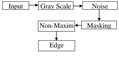
Fig. 3. Edge detection process
The set of processes involved in the applied segmentation model are defined here and also shown in Fig. 3.
Level 1- Smoothing
The initial level of edge detection process extracts the noise from the actual image by the transformation of the raw image to grayscale image through the modification of contrast and brightness, hence blurring of image takes place to eliminate the noise. To perform the elimination of noise in the image, Gaussian filter is widely employed.
Level 2-Identification of Gradients
The edge pixels involve the sharp variation in the gray scale values which are recognized by the computation of image gradients. It is simply a unit vector that pointed out the direction of maximum intensity variation. The vertical and horizontal components of the gradient are determined initially and then the magnitude and the direction of the gradient are determined.
Step-III Non-Maxima Suppression
To carry out the non-maxima suppression, edge thinning is invoked. At this level, based on gradient magnitude, the thick edges in the image are transformed to roughly thin and sharp edges that could be employed for identification processes. At this point, the image undergo scanning process along the detection of the edge and eliminates any pixel value which is not treated to be edge that could leads to the generation of thin line in the output image.
Step-IV Double Thresholding
Two threshold values are assumed in the canny edge
detection method, and
. The pixels with the grayscale values exceeding are strong edge pixels which lead to the outcome of the edge region. The pixels which holds the gray scale values lesser than the threshold are weak edge pixels which leads to the outcome of non-edge region. When the pixels hold the grayscale value in between and , the outcome is based on the nearby pixels.
Step-V Edge Tracking by Hysteresis
Edges which do not link to a definite (strong) edge are eliminated in the ultimate output image. The stronger edges are treated as “Certain Edges” which is involved in the last edge image. The edges which are not stronger ones, however, it is connected to strong edges are involved in the final image.
B. Inception V4 model for classification
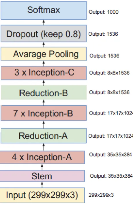
The earlier version of Inception models are used for training in various partitions where every repetitive block is divided into many sub-networks for enabling to fix the entire model in the memory. But, the Inception model can be easily tuned indicating that many possible modifications can be done with respect to number of filters in the distinct layers which does not influence the quality of the fully trained network. For optimizing the speed of the training process, the layer sizes are properly tuned to attain the tradeoff between computations among diverse model sub-networks. Contrastingly, using the TensorFlow (Abadi et al. 2015), latest Inception models is devised with no replica partitioning. It is due to the usage of latest memory optimization to backpropagation, accomplished by cautiously allowing for which tensors are necessary for gradient calculation and structure the computation for minimizing the number of such tensors. Inception-v4 is introduced to drop out the unwanted computation and make regular alternatives for the Inception blocks of every grid size. The overall framework of the Inception-v4 model is depicted in Fig. 4.
Input
image
Gray Scale
image
Noise
Reduction
Masking
Non-Maxim
a
Suppression
Edge
Residual Inception Blocks
For the residual versions of the Inception model, lower Inception blocks are employed compared to actual Inception. Every Inception block follows by a filter-expansion layer that is employed to increase the dimensionality of the filter bank prior to the residual totaling for matching the depth of the input. It is required for compensating the dimensionality cutback tempted via Inception block. Among the various versions of Inception models, the step time of Inception-v4 demonstrated considerably slow, possibly because of many
[image:4.595.187.418.188.541.2]layers. Additional variation among the residual and non-residual Inception models is that batch-normalization is utilized only on top of the conventional layers, however, not on top of the residual summation. It is sensible to anticipate that a comprehensive usage of batch-normalization will be beneficial, however, the design of batch-normalization in TensorFlow consumes more memory and it is required to minimize the total number of layers when batch normalization is employed at any places.
Fig. 4. Inception V4 model
Scaling of the Residuals
It is observed that when the filter count exceeds 1000, the residual versions begins to show instability and the network “died” earlier in the training, implies that the final layer prior to the average pooling has begun to generate only zeros after a several number of iterations. It cannot be avoided by reducing the learning rate or including an extra batch-normalization to this layer. It is also noted that reduction in the residuals prior to appending it to the earlier activation layer is founds to be stabilized in training. Generally, few scaling factors in the range of 0.1 and 0.3 are applied for scaling the residuals prior to appending it to the accumulated layer activations.
III. EXPERIMENTAL RESULTS AND ANALYSIS
A. Dataset details
For highlighting the good characteristics of the presented model, a detailed experimentation takes place on the benchmark ADIAC dataset [11].
The employed dataset has a total of 21 batches with the image count of 1531. In addition, 1412 images with genes and species are present. Furthermore, a set of 70 and 211 classes exist under genus and species classes. This information is provided in Table 1. Next, Table 2 shows the distribution of 70 genus classes in the diatom images. The number of images under
Table 1 Dataset Description
Description Dataset
Total Batches in Dataset 21
Total Number of Images 1531
Total Images with Genus and Species 1412
Number of Genus Class 70
Number of Species Class 211
Table 2 Class Distribution of Genus in Diatom Images
S.No Genus Image Count S.No Genus Image Count
1 Cymatosira 8 36 Fragilaria 33
2 Stauroneis 26 37 Delphineis 32
3 Stenopterobia 2 38 Rhopalodia 3
4 Staurosira 2 39 Meridion 4
5 Epithemia 18 40 Rhaphoneis 9
6 Fallacia 20 41 Cavinula 2
7 Diploneis 18 42 Licmophora 6
8 Psammodiscus 5 43 Tryblionella 6
9 Reimeria 9 44 Hannaea 10
10 Didymosphenia 2 45 Catenula 7
11 Achnanthes 117 46 Stephanodiscus 14
12 Neidium 11 47 Eunotia 42
13 Peronia 15 48 Aneumastus 7
14 Staurosirella 6 49 Ctenophora 3
15 Cocconeis 61 50 Trachysphenia 6
16 Tabularia 7 51 Hyalodiscus 4
17 Thalassiosira 7 52 Opephora 11
18 Synedra 11 53 Rhabdonema 3
19 Cymatopleura 4 54 Craticula 4
20 Frustulia 13 55 Aulacoseira 8
21 Denticula 8 56 Encyonopsis 8
22 Luticola 19 57 Martyana 5
23 Surirella 16 58 Gyrosigma 4
24 Tabellaria 20 59 Rhoicosphenia 6
25 Pseudostaurosira 7 60 Neofragilaria 12
26 Amphora 27 61 Placoneis 13
27 Cymbella 97 62 Odontella 4
28 Navicula 214 63 Brachysira 41
29 Berkeleya 7 64 Stauroforma 4
30 Actinoptychus 5 65 Gomphonema 75
31 Caloneis 17 66 Pinnularia 54
32 Diatoma 21 67 Hantzschia 3
33 Encyonema 33 68 Lyrella 3
34 Thalassionema 8 69 Cyclotella 15
35 Sellaphora 36 70 Nitzschia 53
Fig. 5 shows the sample experimental results attained under the segmentation and classification process of few test images. The first column in the figure shows the original image, the next column illustrates the segmented image and the classified image is provided in third column. From this
Fig. 5. Genus Classification results a) Original Diatom Images b) Segmented Images c) Classified Images
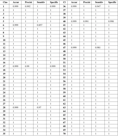
A sample confusion matrix derived for the applied Genus 70 classes are given in Fig. 6. Next, table 3 provides the detailed experimental results attained under every class with respect to accuracy, precision, sensitivity and specificity. Here, the values of these measures should be closer to 1 for better classifier results.
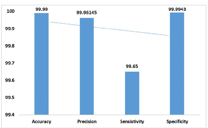
From this table, it is clear that maximum accuracy of 0.999, precision of 0.992, sensitivity of 1 and specificity of 0.999 is achieved under the class 1. Similarly, under the class 2, the presented model shows excellent results with maximum accuracy of 1, precision of 1, sensitivity of 1 and specificity of 1. Likewise, these maximum results are attained under various classes of 3, 4, 5, 7, 8, 9-16, 18-27, 29-35, 37-39, 41-46 and 48-70 respectively. Even though, the results are closer to 0.9 only under rest of the classes. These maximum values attained under different measures clearly exhibited the superior characteristics of the presented model. To further clearly determine the goodness of the presented model, an average analysis of the above-mentioned measures is made as shown in Fig. 7. From this figure, it is stated that a maximum accuracy of 99.99%, precision of 99.96%, sensitivity of 99.65% and specificity of 99.9943% is attained.
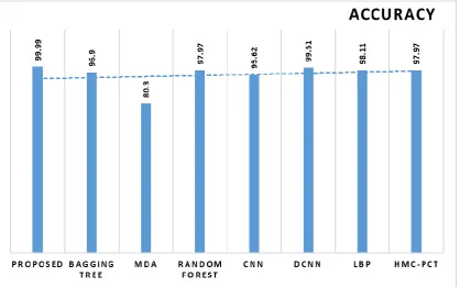
To further point out the optimal results attained by the applied model, a brief comparison is carried out among
diverse methods interms of accuracy. As depicted in the Fig. 8, it is apparent that worst results are attained by MDA model with a least accuracy of 80.3%. In addition, CNN shows moderate results with a high accuracy of 95.62%. At the same time, the bagging tree provides slightly better performance with a higher accuracy of 96.9%.
Table 3 Classification results analysis on diatom dataset
Clas s
Accur acy
Precisi on
Sensitiv ity
Specific ity
Cl ass
Accur acy
Precisi on
Sensitiv ity
Specific ity
1 0.999 0.992 1 0.999 36 0.999 1 0.947 1
2 1 1 1 1 37 1 1 1 1
3 1 1 1 1 38 1 1 1 1
4 1 1 1 1 39 1 1 1 1
5 1 1 1 1 40 0.999 0.991 1 0.998
6 0.999 1 0.857 1 41 1 1 1 1
7 1 1 1 1 42 1 1 1 1
8 1 1 1 1 43 1 1 1 1
9 1 1 1 1 44 1 1 1 1
10 1 1 1 1 45 1 1 1 1
11 1 1 1 1 46 1 1 1 1
12 1 1 1 1 47 0.999 1 0.981 1
13 1 1 1 1 48 1 1 1 1
14 1 1 1 1 49 1 1 1 1
15 1 1 1 1 50 1 1 1 1
16 1 1 1 1 51 1 1 1 1
17 0.999 0.99 1 0.999 52 1 1 1 1
18 1 1 1 1 53 1 1 1 1
19 1 1 1 1 54 1 1 1 1
20 1 1 1 1 55 1 1 1 1
21 1 1 1 1 56 1 1 1 1
22 1 1 1 1 57 1 1 1 1
23 1 1 1 1 58 1 1 1 1
24 1 1 1 1 59 1 1 1 1
25 1 1 1 1 60 1 1 1 1
26 1 1 1 1 61 1 1 1 1
27 1 1 1 1 62 1 1 1 1
28 0.999 1 0.97 1 63 1 1 1 1
29 1 1 1 1 64 1 1 1 1
30 1 1 1 1 65 1 1 1 1
31 1 1 1 1 66 1 1 1 1
32 1 1 1 1 67 1 1 1 1
33 1 1 1 1 68 1 1 1 1
34 1 1 1 1 69 1 1 1 1
Fig. 6. Confusion Matrix of Genus 70 Classes
Fig. 8. Comparison of Accuracy on Proposed with Existing Methods
IV. CONCLUSION
Generally, the usage of widely used diatom indices always needs an exact level of classification that includes time and expert training. This study has introduced a new Inception model for automated diatom image classification model. The presented model involves two main stages namely, canny edge detection based segmentation and Inception model based classification. For highlighting the good characteristics of the presented model, a detailed experimentation takes place on the benchmark ADIAC dataset. To point out the optimal results attained by the applied model, a brief comparison is carried out among diverse methods interms of accuracy. From this figure, it is interesting that the presented model shows extraordinary classification performance with a maximum accuracy of 99.99%, precision of 99.96%, sensitivity of 99.65% and specificity of 99.9943% over the compared methods. In future, the presented model can be further improvised by the inclusion of other deep learning models.
REFERENCES:
1. Mann DG, Vanormelingen P: An inordinate fondness? The number, distributions, and origins of diatom species. J Eukaryot Microbiol 2013, 60(4):414–420.
2. Smol JP, Stoermer EF: The diatoms: applications for the environmental and earth sciences. Cambridge, UK: Cambridge University Press; 2010. 3. Stoermer, E., Smol, J., 2004. The Diatoms: Applications for the
Environmental and Earth Sciences. Cambridge University Press. 4. Susukida, H.; Ma, F.; Bajger, M. Automatic tuning of a graph-based
image segmentation method for digital mammography applications. In Proceedings of the 5th IEEE International Symposium on Biomedical Imaging: From Nano to Macro, Paris, France, 14–17 May 2008; pp. 89–92
5. Bueno, G.; Deniz, O.; Pedraza, A.; Salido, J.; Cristobal, G.; Saul, B. Automated Diatom Classification (Part A): Handcrafted feature approaches. Appl. Sci. 2017, in press.
6. Dimitrovski, I.; Kocev, D.; Loskovska, S.; Dzeroski, S. Hierarchical classification of diatom images using ensembles of predictive clustering trees. Ecol. Inform. 2012, 7, 19–29.
7. Krizhevsky, A.; Sutskever, I.; Hinton, G. Imagenet classification with deep convolutional neural networks. In Advances in Neural Information Processing Systems; Neural Information Processing Systems Foundation, Inc.: La Jolla, CA, USA, 2012; pp. 1097–1105.
8. Szegedy, C.; Liu,W.; Jia, Y.; Sermanet, P.; Reed, S.; Anguelov, D.; Erhan, D.; Vanhoucke, V.; Rabinovich, A. Going deeper with convolutions. In Proceedings of the IEEE Conference on Computer Vision and Pattern Recognition, Boston, MA, USA, 7–12 June 2015; pp. 1–9.
9. Maiti, I. and Chakraborty, M., 2012, November. A new method for brain tumor segmentation based on watershed and edge detection algorithms in HSV colour model. In 2012 NATIONAL CONFERENCE ON COMPUTING AND COMMUNICATION SYSTEMS (pp. 1-5). IEEE. 10.Szegedy, C., Ioffe, S., Vanhoucke, V. and Alemi, A.A., 2017, February. Inception-v4, inception-resnet and the impact of residual connections on learning. In Thirty-First AAAI Conference on Artificial Intelligence.
11.https://rbg-web2.rbge.org.uk/ADIAC/pubdat/downloads/public_images.