An Automatic Classification of Dermoscopy Image with Multilayer Perceptron using Weka



Abstract: Skin cancer a distressing disease (or) an abnormality. The growth starts from the human body’s epidermis. Skin cancer treatments depend primarily upon the sign and location of the tumour. Computerized image analysis influences the accurate assessment of skin cancer in an effective manner. Skin cancer affects people in various parts of the body. A computer method on the pigment skin image should be examined to diagnose the skin cancer precisely. This is the dermatologist’s pre-screening system for early diagnosis. The associated and the proposed work is compared and examined. The proposed work gives the report on the classification of lesions from the dermoscopy images with basic steps such as pre-processing and classification. Here GLCM and Multilayer Perceptron analysis is used to differentiate the features. The simulation measures the accurate diagnosis of the image of ground truth and the segmented image and confirms the accuracy values up to 98% for Classification.

Keywords : Weka, Disceretize, Multilayer Perceptron, GLCM, Training.

I. INTRODUCTION

The random and massive growth of anomalous skin cells is skin cancer. It occurs when the disease cell damage causes genetic defects that lead to rapid multiplication of skin cells malignant tumour formation. Primarily, cancer cells form in the sun-exposed skin areas such as scalp, face, lips, ear, neck, chest, arms and bands and women’s legs [7,8]. But the rarely skin-exposed areas like your palms, under your finger nails or toe nails and the genital areas can also be proving to cancer cells. Melanoma occurs in people with dark skin tones (ie) it occurs mostly in areas that are not normally exposed to sun such as hand palms and foot soles. A mole is a benign growth of melanocytes, the colour of the skin. Though very few moles develop cancer, a typical mole can develop over time into melanoma [9, 10]. Normal moles can appear flat or raised or they can start flat and grow overtime. The disease starts from the human body’s epidermis.

Yanjun Peng proposed an advasial network as segmentation architecture and constructs the network using Unet with convolutional layer [1]. The dataset used here is PH2 and ISBI 2016. The network is trained eith segmentation architecture to learn about the distribution of training data. Here they use back propogation network for depth trained, with respect to loss function by segmentation network and discrimination network.

Imene Khanfir have proposed a contextual architecture of spatial knowledge to segment skin lesions [2]. The fuzzy and

Revised Manuscript Received on October 05, 2019.

* Correspondence Author

Dr. N. Angel*, Department of CSE, St. Joseph’s College of Engineering, Chennai, India. Email: [email protected]

K. Sudha, Department of CSE, St. Joseph’s College of Engineering, Chennai, India. Email: [email protected]

means, measures the full contextual pixel information. This algorithm segments the image if pixel values are of low quality. Contextual pixel contains, low quality values that describe the local possibility distribution information in its entirely. Spatial knowledge based on pixels is split into sectors. The initial sector creates the segmentation scene and trains the raw data. The next level is the intermediate level that extracts pixel value knowledge. Next sub-semantic level identifies the function of possibilities and distribution as probability and function of mass.

Saranya raj has proposed a deeply convolutionary neutral network to focus on mammographic image analysis [3]. For processing, multilayer perception is used. The processing states begin with bilateral vector grid filtering to segment the image contour and calculate after noise filtering. The architecture is divided into five stages, such as crop and

resize, de-noise, train classify, evaluate

classification-characteristics. The feature extracted is area, perimeter, radius, smoothness. Confusion matrix is constructed to divide regions for extracting characteristics.

Tomas Majtner had extracted a feature set from deep learning models, an optimized deep learning was proposed [4]. The melanoma is detected by linear discriminate analysis (LDA) after the learning process. The LDA reduces the size of space. Various metrics such as SVM, KNM, discriminate analysis, Bayes Classifier evaluate the work. The algorithm is built on the dataset of ISIC.

Christine Fink had suggested a smart match algorithm to find a chamfer distance function that is obtained after psoriasis severity scoring by area of psoriasis and severity index [5]. EDT algorithm analyses the entire body surface, but the skin surface regions are calculated using DOBDIS formula and Wallac's "nice rule". The features such as redness, thickness and scalability are finally found.

Monisha have suggested a CAD algorithm with recognition gadget using ANN that finds the pattern set of affected regions symptoms [6]. The pattern consists of skin rashes and skin redness. GLCM features are generated for classification and combined for efficient classification with probabilistic neural network.

II. MATERIALS AND METHOD

A. GLCM

Grey Level Co-Occurrence Matrix (GLCM) is a standout amongst the best known surface Analysis strategies.

GLCM gauges picture properties identified with second request measurements. Every section (i,j) in GLCM relates to the quantity of events of the pair of dark dimensions [11].

An Automatic Classification of Dermoscopy

Image with Multilayer Perceptron using Weka

A measurable technique for inspecting surface that considers the spatial relationship of pixels is the Grey Level Co-Occurrence Matrix (GLCM), otherwise called dimension spatial reliance framework. The GLCM describe the surface of a picture by ascertaining how frequently combines of pixel with explicit qualities and in a predefined spatial relationship happen in a picture, making a GLCM, and after that extricating factual measures from this grid [12, 13]. A co-event grid is a square lattice with components comparing to the general recurrence of Occurrence of sets of dark dimension of pixels isolated by a specific separation in a provided guidance..

B. Entropy

Entropy estimates the confusion of a picture and it accomplishes its biggest esteem when all components in network are equivalent [14]. At the point when the picture isn't texturally uniform numerous GLCM components have exceptionally little qualities, which infer that entropy is extremely huge. Hence, entropy is contrarily relative to GLCM vitality.

Entropy= (1)

Contrast:

Difference includes a proportion of the picture differentiate or the measure of neighborhood varieties present in a picture [15].

Contrast = (2)

C. Angular Second Moment

Energy, likewise called Angular Second Moment and Uniformity is a proportion of textural Uniformity of a picture. Energy achieves its most elevated esteem when dimension conveyance has either a steady or an intermittent structure [16]. A homogenous picture contains not many predominant dimension tone advances and consequently the network for this picture will have less sections of bigger greatness bringing about extensive incentive for energy include. Interestingly if the lattice contains an expansive number of little sections, the energy highlight will have a littler esteem. Angular Second Moment = (3)

D. Inverse Difference Moment

Inverse contrast minute estimates picture homogeneity. This parameter accomplishes its biggest esteem when a large portion of the events in GLCM are focused close to the fundamental corner to corner [17]. IDM is contrarily corresponding to GLCM differentia.

Inverse Difference Moment = (4)

E. MULTI LAYER PERCEPTRON

A multilayer perceptron (MLP) is a class of feed forward fake neural system. A MLP comprises of, no less than, three layers of hubs: an info layer, a concealed layer and a yield layer. With the exception of the information hubs, every hub is a neuron that utilizes a nonlinear enactment work [18, 19]. MLP uses a regulated learning method called back

propagation for training. Its numerous layers and non-straight actuation recognize MLP from a direct perceptron. It can recognize information that isn't directly separable.

Activation function

In the event that a multilayer perceptron has a direct enactment work in all neurons, that is, a straight capacity that maps the weighted contributions to the yield of every neuron, at that point direct variable based math demonstrates that any number of layers can be decreased to a two-layer input-yield display. In MLPs a few neurons utilize a nonlinear actuation work that was created to show the recurrence of activity possibilities, or terminating, of natural neurons.

The two regular enactment capacities are both sigmoids, and are depicted by

and (5)

The first is a hyperbolic digression that ranges from - 1 to 1, while the other is the calculated capacity, which is comparable fit as a fiddle however runs from 0 to 1. Here yi is the yield of the ith hub (neuron) and vi is the weighted total of the information associations. Elective initiation capacities have been proposed, including the rectifier and softplus capacities.

Learning

Learning happens in the perceptron by changing association loads after each bit of information is prepared, in view of the measure of mistake in the yield contrasted with the normal outcome [20]. This is a case of administered learning, and is helped out through back propagation, a speculation of the least mean squares calculation in the direct perceptron. Output node error :

)

(

)

(

)

(

n

d

n

y

n

e





(6)

Weights of the node are corrected that decrease the resultant

(7)

By applying gradient descent , the change in each weight is

(8) Yi is the result of previous neuron, is the rate of learning

The function to be calculates is based on the local field induced vj, simple way to indicate that for output node this function is facilitate to

- (∂∈(n))/(∂v_i (n))= e_i (n) ∅^' (v_i (n)) (9)



(10)

Terminology

The expression "multilayer perceptron" does not allude to a solitary perceptron that has various layers. It contains numerous perceptrons that are sorted out into layers. MLP "perceptrons" are not perceptrons in the strictest conceivable sense [21]. Genuine perceptrons are formally an uncommon instance of fake neurons that utilization an edge enactment capacity.

III. PROPOSED SYSTEM Algorithm

Step 1 : Input RGB image K(x,y) and Generate Binary image BT(x,y).

Step 2 : Generate GLCM properties of BT(x,y) to extract features.

Step 3 : Convert the extracted features in a proper class file.

Step 4 : Discretize the class file into a Nominal file. Step 5 : Use Multilayer Perceptron with Training and Percentage Split.

Step 6 : Training set trains the features values to manipulate among itself.

Step 7 : Percentage split is set to 50%.

Step 8 : Margin curve and threshold curve describes the outcomes.

Step 9: Confusion matrix is constructed to display the maximum accuracy.

Architecture Diagram

Fig 1.Architecture Diagram of Proposed System

IV. RESULTS

The input RGB dermoscopy image is taken from dermquest dataset. The input image is converted into binary image. The binary image is taken on input for feature extraction. The feature extraction on binary image derives plenty of parameter using GLCM. The GLCM verifies the image as gray scale and the co-occurrence matrix. The experimental work was done using matlab2015.

Fig 2. Pre-Processing the Input data

The parameters of GLCM are entropy, contrast, angular second moment and inverse difference moment. The entropy measures the confusion property of image. The contrast measures the neighbourhood property. The angular second moment is also called as energy, derives textural uniform property of image. The inverse difference moment derives the image homogeneity the data which are retrieved are numeric data in decimal format. The numerical data is taken into weka tool which supports plenty of classification function. The obtained data should be filtered to nominal value. Hence the data is imported into weka tool for pre-processing. The pre-processing is done to filter the unwanted data and to convert the data into nominal. It is converted by the function called Discretize. The data is discretize into set of nominal or segregated values. After converting the data into nominal the field of data are visualized in Fig. 2.

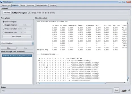
Fig 3. Classification of Input data using Multilayer Perceptron

Test mode: evaluate on training data Time taken to build model: 19.86 seconds

Time taken to test model on training data: 0.06 seconds

=== Summary ===

Correctly Classified Instances 196 98 % Incorrectly Classified Instances 4 2 % Kappa statistic 0.9733

Mean absolute error 0.0058 Root mean squared error 0.0536 Relative absolute error 3.8431 % Root relative squared error 19.5865 % Total Number of Instances 200

Next the classification functionality is brought to distinguish the nominal data. The multilayer perceptron is used to classify nominal data by comparing the attributes. The attribute used here is userid as name of the image, contrast, correlation, energy, homogeneity and outcomes which are derived from GLCM.

Table 1. Summary Classification of Input data using Multilayer Perceptron

The MLP divides the data into n number of perceptrons each perceptron percept with each attribute of data and compared with each other to find the best outcomes shown in Fig 3.

=== Confusion Matrix ===

a b c d e f g h i j <-- classified as

45 0 0 0 0 0 0 0 0 0 | a = '(-inf-166567.043864]'

0 76 0 1 0 0 0 0 0 0 | b = '(166567.043864-282831.604768]' 0 0 14 1 1 0 0 0 0 0 | c = '(282831.604768-399096.165672]' 0 1 0 40 0 0 0 0 0 0 | d = '(399096.165672-515360.726576]' 0 0 0 0 6 0 0 0 0 0 | e = '(515360.726576-631625.28748]' 0 0 0 0 0 8 0 0 0 0 | f = '(631625.28748-747889.848384]' 0 0 0 0 0 0 6 0 0 0 | g = '(747889.848384-864154.409288]' 0 0 0 0 0 0 0 0 0 0 | h = '(864154.409288-980418.970192]' 0 0 0 0 0 0 0 0 0 0 | i = '(980418.970192-1096683.531096]' 0 0 0 0 0 0 0 0 0 1 | j = '(1096683.531096-inf)'

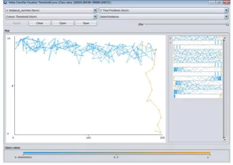
Fig 4. Margin Curve of Classification

The MLP classification functionality requires some test option. The test options are training set and percentage split. The input data is divided into training set and test set as per the percentage split on the data. The percentage split is given as 50% hence the data is divided into two. The first half is used for training and the next half is used for testing the data. After completion of classification a marginal curve is generated to display the margin layer of contrast attribute. The class contrast is segregated from -1 to +1 with the mid value of -0.000 to 1 on x axis and the length of the margin curve extends up to 200 on y axis.

For each instances on contrast attribute each object is compared to all other objects to form a group of instances , that proves the efficiency of classification The margined curve describes the formation of contrast attribute lies in the same region along x=1 and y =0 to 200. The value of x lies on the same line and hence the classification is made completely perfect shown in Fig 4.

Fig 5. Threshold curve of classification

Fig 6. Cost Benefit Analysis of classification

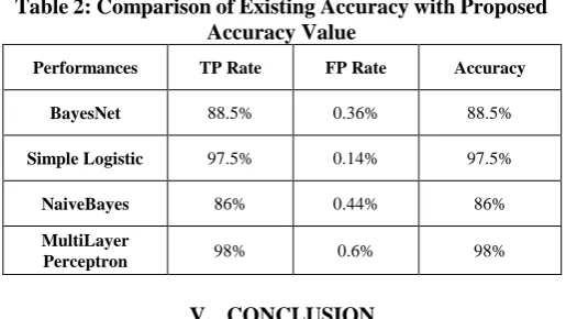
The cost benefit analysis is generated between the class variable and true positive values. The differentiation of values is given by different threshold color. The confusion matrix is constructed between 2 predictions. The classification accuracy is obtained up to 99% is shown in Fig 6. After completing the proposed work, the accuracy is compared with the existing work and describes in Table 2.

Table 2: Comparison of Existing Accuracy with Proposed Accuracy Value

Performances TP Rate FP Rate Accuracy

BayesNet 88.5% 0.36% 88.5%

Simple Logistic 97.5% 0.14% 97.5%

NaiveBayes 86% 0.44% 86%

MultiLayer

Perceptron 98% 0.6% 98%

V. CONCLUSION

After a fine extraction of features for classification, GLCM terminates by generating parameters to create a class for weka. The Discretize function converts the GLCM features to a nominal data. The nominal data is visualized to display the segregation ratio of attributes. Multilayer perceptron percept’s its given nominal data into multi perception and compares all perceptron to each other to give the best outcomes. The nominal data is contrast attribute of image, comprises on comparison of each data. Finally balanced data is taken into percept with other attribute. The margin curve provides the perfect visualisation of margin and instances. The threshold curve visualizes the range of threshold of each value of nominal attribute. Finally the cost benefit analysis describes the perfect efficiency up to 98% of classification.

REFERENCES

1. Yanjun Peng, Ning Wang, Yuanhong Wang & Meiling Wang, "Segmentation of dermoscopy image using adversarial networks", Multimedia Tools and Applications (2018).

2. .Imene Khanfir Kallel, Shaban Almouahed, Bassem Alsahwa & Basel Solaiman," The use of contextual spatial knowledge for low-quality image segmentation", Multimedia Tools and Applications (2018). 3.Saranyaraj D., Manikandan M. & Maheswari S.." A deep convolutional

neural network for the early detection of breast carcinoma with respect to hyper- parameter tuning", Multimedia Tools and Applications (2018).

4.Tomas Majtner, Sule Yildirim-Yayilgan & Jon Yngve Hardeberg, "Optimised deep learning features for improved melanoma detection", Multimedia Tools and Applications (2018).

5.Christine Fink, Tobias Fuchs, Alexander Enk & Holger A. Haenssle, "Design of an Algorithm for Automated, Computer-Guided PASI Measurements by Digital Image Analysis", Journal of Medical Systems (2018).

6.M. Monisha, A. Suresh & M. R. Rashmi,"Artificial Intelligence Based Skin Classification Using GMM", Journal of Medical Systems (2019). 7.Jose Fernandez Alcon, calinaCiuhu, Warner ten Kate, Adrienne

Heinrich, Natallia Uzunbajakava, GertruudKrekels, Denny Siem, and Gerard de Haan, “Automatic Imaging System with Decision Support for Inspection of Pigmented Skin Lesions and Melanoma Diagnosis”, IEEE Journal Of Selected Topics In Signal Processing, Vol 3, No 1, 2009. 8.B. Bozorgtabar, S. Sedai, P. Kanti Roy, R. Garnavi , “Skin lesion

segmentation using deep convolution networks guided by local unsupervised learning”, IBM J. RES. & DEV.61,2017.

9.FaouziAdjed, Syed Jamal SafdarGardezi, FakhreddineAbabsa, IbrahimaFaye ,Sarat Chandra Dass , “Fusion of structural and textural features for melanoma recognition”, IET Computer Vision 2018, Vol 12, No 2.

10. N C F. Codella, Q.-B. Nguyen, S. Pankanti, D. A. Gutman, B. Helba, A. C. Halpern, J. R. Smith, “Deep learning ensembles for melanoma recognition in dermoscopy images”, IBM J. RES. & DEV.61 (5), 2017. 11. HaraldGanster, Axel Pinz, ReinhardRöhrer, Ernst Wildling, Michael Binder, and HaraldKittler,”Automated Melanoma Recognition, IEEE Transactions On Medical Imaging, Vol 20, No 3, 2001.

12. SaptarshiChatterjee, DebangshuDey, SugataMunshi , “Optimal selection of features using wavelet fractal descriptors and automatic correlation bias reduction for classifying skin lesions.”, Biomedical Signal Processing and Control 2018.

13. Steven Schoenecker ,TodLuginbuhl,”Characteristic Functions of the Product of Two Gaussian Random Variables and the Product of a Gaussian and a Gamma Random Variable”, IEEE Signal Processing Letters, Vol 23, No 5, 2016.

14. Peng-Lang Shui , Li-Xiang Shi , Han Yu , Yu-Ting Huang,”Iterative Maximum Likelihood and Outlier-robust Bipercentile Estimation of Parameters of Compound-Gaussian Clutter With Inverse Gaussian Texture”, IEEE Signal Processing Letters, Vol 23, No 11, 2016. 15. MiladNiknejad, Isfahan, HosseinRabbani ,

MassoudBabaie-Zadeh,”Image Restoration Using Gaussian Mixture Models With Spatially Constrained Patch Clustering”, IEEE Transactions on Image Processing, Vol 24, No 11, 2015.

16. Lucas P. Queiroz , Francisco Caio M. Rodrigues , Joao Paulo P. Gomes , Felipe T. Brito , Iago C. Chaves , “A Fault Detection Method for Hard Disk Drives Based on Mixture of Gaussians and Nonparametric Statistics”, IEEE Transactions on Industrial Informatics, Vol 13, No 2, 2017.

17. EwedaEweda , Neil J. Bershad , José Carlos M. Bermudez,”Stochastic Analysis of the LMS and NLMS Algorithms for Cyclostationary White Gaussian and Non-Gaussian Inputs”, IEEE Transactions on Signal Processing, Vol 66, No 18, 2018.

18. Wen Wang , Ruiping Wang , Zhiwu Huang , Shiguang Shan , Xilin Chen,” Discriminant Analysis on Riemannian Manifold of Gaussian Distributions for Face Recognition With Image Sets”, IEEE Transactions on Image Processing, Vol 27, No 1, 2018.

19. M. Yusaf , R. Nawaz , J. Iqbal,”Robust seizure detection in EEG using 2D DWT of time- frequency distributions”, Electronics Letters, Vol 52, No 11,2016.

20. ThamizharasiAyyavoo, Jayasudha John Suseela,” Illumination pre-processing method for face recognition using 2D DWT and CLAHE”,IET Biometrics , Vol 7, No 4, 2018.

22. AmanGhasemzadeh, Hasan Demirel,”3D discrete wavelet transform-based feature extraction for hyperspectral face recognition”, IET Biometrics, Vol 7, No 1, 2018.

23. Wolfgang Schnurrer , NiklasPallast , Thomas Richter , Andre Kaup,”Temporal Scalability of Dynamic Volume Data Using Mesh Compensated Wavelet Lifting”, IEEE Transactions on Image Processing, Vol 27, No 1, 2018.

24. Y. Zhang , T. Y. Ji , M. S. Li , Q. H. Wu,”Identification of Power Disturbances Using Generalized Morphological Open-Closing and Close-Opening”, IEEE Transactions on Industrial Electronics, Vol 63, No 4, 2016.

25. Sung-JeaKo , A. Morales , Kyung-HoonLee,”Block basis matrix implementation of the morphological open-closing and close-opening”, IEEE Signal Processing Letters, Vol 2, No 1,1995. 26. Sung-JeaKo , A. Morales , Kyung-Hoon Lee,” A fast implementation algorithm and a bit- serial realization method for grayscale morphological opening and closing”, IEEE Transactions on Signal Processing, Vol 43, No 12, 1995.

27. Kyung-HoonLee , A. Morales , Sung-JeaKo,”Adaptive basis matrix for the morphological function processing opening and closing”, IEEE Transactions on Image Processing ( Vol 6 , No 5 , May 1997, pp: 769 – 774.

28. NingMa ,Jian xin Wang,”Dynamic threshold for SPWVD parameter estimation based on Otsu algorithm”, Journal of Systems Engineering and Electronics, Vol 24, No 6,2013.

29. G.Y. Zhang , G.Z. Liu , H. Zhu , B. Qiu,” Ore image thresholding using bi-neighbourhood Otsu's approach”, Electronics Letters, Vol 46, No 25, 2010.

30. Jing-Hao Xue , D. Michael Titterington,” t-Tests,F-Tests and Otsu's Methods for Image Thresholding”, IEEE Transactions on Image Processing , Vol 20, No 8, 2011.

31. A.K. Khambampati , D. Liu , S. K. Konki , K. Y. Kim,” An Automatic Detection of the ROI Using Otsu Thresholding in Nonlinear Difference EIT Imaging”, IEEE Sensors Journal, Vol 18, No 12, 2018. 32. P. Bao , Lei Zhang , XiaolinWu,”Canny edge detection enhancement by

scale multiplication”, IEEE Transactions on Pattern Analysis and Machine Intelligence , Vol 27, No 9, 2005.

33. Y. Zhang , P.I. Rockett,” The Bayesian Operating Point of the Canny Edge Detector”, IEEE Transactions on Image Processing, Vol 15, No 11, 2016.

34. A. Prabhu Chakkaravarthy & A. Chandrasekar,"An Automatic Segmentation of Skin Lesion from Dermoscopy Images using Watershed Segmentation", 2018 International Recent Trends in Electrical, Control and Communication (RTECC), pp. 15-18.

AUTHORSPROFILE

Angel N, received her PhD in Manonmainam Sundaranar University Tirunelveli, M.E(CSE) degree from Sathyabama University, MCA degree from Standard Fireworks College for Women affiliated to Madurai Kamaraj University. She is currently working as a Associate Professor in the Department of Computer Science and Engineering in St.Joseph’s College of Engineering, Chennai. Her area of interest includes Web Security, Advanced Java Programming, Service Oriented Architecture.