Abstract: Paper describes the technique of parallelization of data mining algorithms based on the block structure. The described technique takes into account the characteristics of the execution environment of parallel algorithms, such as the distribution of the analyzed data, as well as the features of the parallelized algorithm.
Keywords : Data mining, parallel algorithms, block structure.
I. INTRODUCTION
In the last few years, an increase in the productivity of computer technology is associated with the development of multi-core processors. Such processors are no longer the prerogative of powerful computing servers. Processors with four, six, or eight cores are equipped with ordinary home, office, and even more so analyst jobs. However, modern software significantly lags behind the hardware and often inefficiently uses the provided hardware resources. Typically, computers with multi-core processors use two or at best, four cores. This problem is primarily associated with the complexity of the task of parallelizing computational algorithms. Unfortunately, data mining algorithms are no exception. Most of the efforts of researchers in the field of parallel data mining algorithms are spent on parallelization of individual analysis algorithms and their further optimization [1, 2]. The situation is aggravated by the fact that these efforts are applied on the basis of a certain computing environment, therefore, when such a solution is transferred to other conditions, it becomes ineffective.
This paper proposes a technique for parallelizing data mining algorithms. It describes a sequence of steps for parallelizing any data mining algorithm implemented in a block structure [3]. This takes into account both the execution environment of the algorithm and the type of data distribution, as well as the features of such algorithms.
II. PROPOSEDAPPROACH
The initial data for the parallelization technique of the data mining algorithm are:
• Description of the execution environment of the parallel algorithm:
Revised Manuscript Received on December 05, 2019.
Karshiev Zaynidin, Samarkand branch of the Tashkent University of Information Technologies named after Muhammad al-Khwarizmi, Uzbekistan.
Sattarov Mirzabek, Samarkand branch of the Tashkent University of Information Technologies named after Muhammad al-Khwarizmi, Uzbekistan.
the number of processors (threads) on which parallel execution is possible;
processor performance;
presence / absence of shared memory among processors and / or means of interaction;
• Type of distribution of the analyzed data [2]:
single or distributed storage;
in the case of distributed storage, the type of distribution: horizontal or vertical;
• Description of the data mining algorithm:
formal description of data mining;
knowledge model obtained as a result of the algorithm.
The paper [4] describes the classification of parallel data mining algorithms. In accordance with it, two levels of characteristics of such algorithms are distinguished:
structural level - suggesting a change in the structure of the parallel algorithm;
customizable level - which involves changing the parameters of the parallel algorithm by setting it without changing the structure of the algorithm.
In accordance with this classification, we divide the technique into two main stages:
I. determining the structure of a parallel data mining algorithm;
II. setting up a parallel data mining algorithm.
At the first stage, the structure of the data mining algorithm is analyzed in order to identify typical elements and other features inherent in the algorithm. Based on the results of the analysis, a parallel algorithm structure is formed.
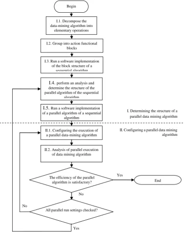
To determine the structure of a parallel algorithm, you must perform the following steps:
I.1. decompose the data mining algorithm into elementary operations;
I.2. group actions that perform discrete model changes into functional blocks;
I.3. perform software implementation of the block structure of a sequential algorithm;
I.4. analyze the resulting structure taking into account the remaining cycles and conditional transitions and determine the structure of the parallel algorithm; I.5. perform software implementation of the parallel
structure of the data mining algorithm based on
previously implemented functional blocks.
At the first step, the structure of the algorithm should be decomposed into elementary operations that are performed on the knowledge model: adding, deleting, and changing individual elements of the
model (in accordance with the formal algorithm model
Technique of Building Parallel Data Mining
Algorithms
described in [5]). At the same time, the main control structures should be clearly distinguished in the structure of the algorithm: cycles, conditional transitions, etc. Decomposition should be performed taking into account the following conditions:
after completing each operation, the integrity of the knowledge model is maintained;
the number of variables used by various operations should be minimized and localized (variables should be used only for consecutive operations).
At this step, the presence of elementary operations that do not change the knowledge model is allowed.
An example of such a decomposition is the following pseudo-code of the Naive Bayes algorithm (for a data set with a single target attribute):
1.for i=1 to |W| // for all vectors
2.p = D(at).getIndex(vt.i) // get the index of the value of the
target attribute at of the current vector from its domain of
definition D(at)
3.Mnb.kp= Mnb.kp+1
4.for j=1 to |A| // for all independent attributes
5.u = Mnb.R.getIndex((aj = vj.i) (at = vt.p) ) // get the index
of the rule with the corresponding conditional and target parts
6.Mnb.nu = nu + 1
7.end for j;
8.end for i;
The given Naïve Bayes algorithm computes the elements of the Mnb model corresponding to the NaveBayesModel model of the PMML standard [6], formally described in the article [7] and including the following elements:
Mnb.R – is the set of classification rules of the form (aj
= vj.i) (at = vt.p);
Mnb.kp – the number of vectors for which the value of
the target attribute vt.i;
Mnb.nu – the number of vectors for which the
independent attribute aj has the value vj.i and the target attribute at has the value vt.p.
The described algorithm works with the original knowledge model, in which all elements are already created based on metadata about the data being processed (values of the target and non-target attributes). In this regard, the algorithm does not have operations related to adding elements to the model, and there are only operations to change them in lines 3 and 6. Actions in lines 2 and 5 do not change the model. In addition, the algorithm includes two cycles nested into each other: an external one - for all vectors W and an internal one - for all independent attributes of A.
The second step is the grouping of actions into functional blocks that perform discrete changes in the knowledge model. In the process of grouping into a functional block, operations related to each other by common local variables are distinguished. The basic in such blocks are operations that change the state of the knowledge model, to which are added the previous and / or subsequent operations that do not change the model. The grouping of operations that do not change the model with related basic operations is performed on the basis of their logical belonging to them. A sign of such a logical
connection may be the use of intermediate (local) variables. Such variables must be localized inside the created function block.
Control structures (cycles, conditional transitions, etc.) do not change the state of the model, however, they must be allocated to separate control blocks.
In our example, there are two operations that change the knowledge model (lines 3 and 6). They should form two functional blocks:
IncForTargetValue – incrementing the number of vectors with a specific value of the target attribute Mnb.kp;
IncForRule – incrementing the number of vectors corresponding to a certain rule Mnb.nu.
The operation from line 2 should be added to the IncForTargetValue block, because it uses the common intermediate variable p with the basic operation on line 3. The operation from line 5 should be added to the IncForRule block for the same reasons.
In addition to functional blocks in the algorithm, two control blocks can be distinguished:
CycleByVector – cycle through all vectors of the data set;
CycleByAttribute – cycle through all independent attributes.
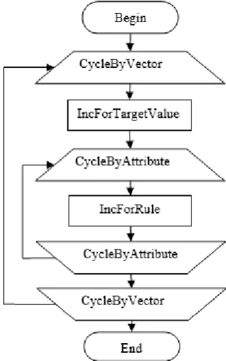
[image:2.595.338.503.386.649.2]Thus, the previously described Naïve Bayes algorithm can be represented as a block diagram depicted in Figure 1.
Fig. 1. Block diagram of Naïve Bayes algorithm At the third step, it is necessary to implement the implementation of the functional blocks. This implementation should be performed by inheriting from the base classes described in the monograph [3]. The resulting functional blocks must be combined into a single sequential algorithm.
At the penultimate step of the first stage of the technique, it is necessary to analyze the
algorithm. The result of this analysis should be the structure of a parallel algorithm, assigned to one of the classes in accordance with the proposed classification [4]. The following recommendations can be made:
if there is a cycle along vectors in the structure, then data parallelization is possible, while the parallel branches of the algorithm will be the cycle itself with a selected portion of vectors and blocks running inside the cycle and processing them;
when selecting parallel branches in the algorithm whose work needs to be coordinated (for example, distributing vectors between branches depending on the value of the target attribute), a dispatcher stream can be added to the structure;
if a conditional branch block is present in the structure, then parallelization by tasks is possible; in addition, the conditional branch itself and the blocks preceding it can be allocated to the dispatcher flow, and blocks that are executed depending on the condition being fulfilled by parallel branches;
if the algorithm contains blocks that require processing of all data (for example, comparing each vector with each or calculating a function for all vectors), then it is possible to implement interaction between flows or add a dispatcher stream containing blocks for routing vectors;
if the algorithm builds a knowledge model that cannot be correctly combined after its completion and requires coordination at intermediate stages (for example, to construct decision trees that are built for different sets of data, an intermediate agreement on the information content of the attributes must be performed), then the algorithm structure may stream manager will be added.
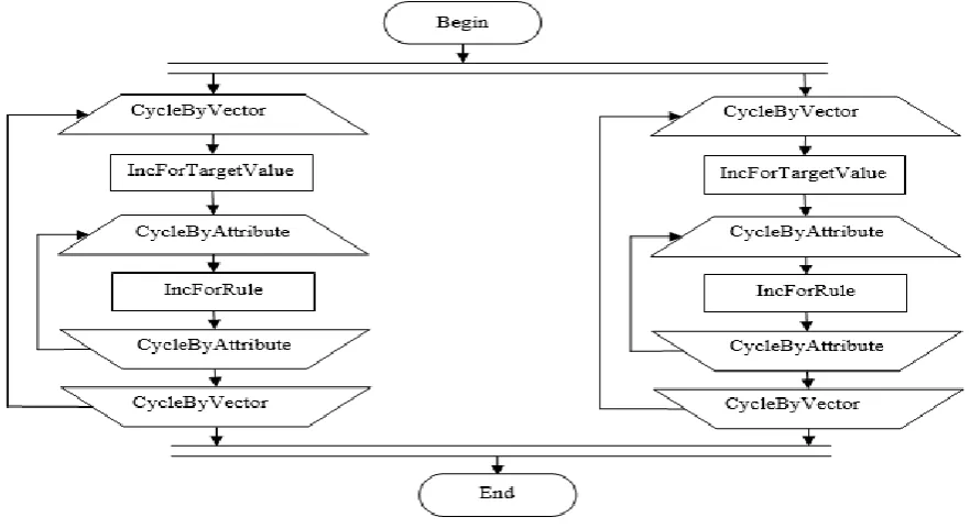
In our example, when analyzing the structure of the algorithm shown in Figure 1, we can conclude that it can be
parallelized using data, due to the presence of a cycle of vectors in it — CycleByVector. At the same time, in the parallel branches of the algorithm, the CycleByVector block and all blocks running inside this cycle will be executed.
The resulting parallel algorithm structure is shown in Figure 2.
At the last step, the implementation of the parallel algorithm of the selected structure is performed. In this case, the implementation is performed by adding to the serial version of the algorithm (obtained in step I.3) the corresponding blocks for parallel execution described in the monograph [3].
At the second stage of parallelization of the algorithm, the execution of the parallel algorithm is configured and its efficiency is analyzed, followed by debugging. The stage includes the following steps:
II.1. Configuring the execution of a parallel data mining algorithm in accordance with environmental parameters and the type of data distribution;
II.2.analysis of the parallel execution of the data mining algorithm on test data, by evaluating the effectiveness and acceleration;
a. return to step II.1. if the results are unsatisfactory and not all settings have been tested;
[image:3.595.67.508.469.709.2]return to step I.4 if the results are unsatisfactory and all settings have been tested.
Fig 2. Parallel Naïve Bayes algorithm structure At the first step of the second stage, the execution of the
parallel algorithm is performed:
- indicates the means of executing the parallel algorithm (threads, service-oriented
existing capabilities and the execution environment;
-the number of handlers of parallel branches of the algorithm is indicated, depending on the runtime (for example, on the number of cores on the processor);
-indicates the type of parallel execution of the data mining algorithm [4]:
-SDSM - single data stream and single model;
-MDSM - multiple data streams and single model;
-SDMM - single data stream and multiple models;
-MDMM - multiple data streams and multiple models.
Setting the type of parallel execution of the algorithm can be performed depending on the type of data distribution, the
features of the knowledge model under construction and the execution environment. At this step, you can give the following recommendations:
-if the source of information is single, then it is preferable to choose the type SD *, if there are several sources then MD *;
-if the knowledge model is not combined from several independently constructed and the execution tools have
a common memory, then the best option would be to
select * SM type, otherwise any type can be used. In the next step, it is necessary to measure the running time of the serial and parallel algorithms. Based on the measurements, calculate the acceleration and performance of
the constructed parallel data mining algorithm. If the obtained estimates do not satisfy, then you can return to the previous step and choose another type of parallel algorithm execution. If changing the type of execution of the parallel algorithm
does not allow increasing the efficiency of the algorithm to the required level, then you can return to the penultimate step of the first stage and restructure the algorithm from the implemented functional blocks (without changing the blocks
themselves).
Fig 3. Block diagram of technique for buliding parallel data mining algorithms III. RESULTSANDDISCUSSIONS
In accordance with the technique, experiments were performed on the Naïve Bayes algorithm. Threads are selected as a means of execution, a parallel program runs on a
4-core Intel (R) Core (TM) i7-2600 processor @ 3.40 GHz 3.40 GHz and 4 GB of RAM. It executed in four versions:
for data with the number of vectors 150;
for data with the number of vectors 1500;
for data with the number of vectors 3000;
for data with the number of vectors 6000;
From Table 1 it can be seen that parallel execution of the algorithm for data with the number of vectors 150, 1500, 3000 and 6000 gave effective results with MDSM and MDMM.
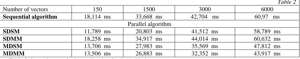
In order to obtain even more effective results, in accordance with the steps of the technique, the parallel Naïve Bayes algorithm was restructured and we obtain the following results (Table 2):
Table 1
Number of vectors 150 1500 3000 6000
Sequential algorithm 18,114 ms 33,668 ms 42,704 ms 60,97 ms
Parallel algorithm
SDSM 18,665 ms 31,919 ms 41,446 ms 58,316 ms
SDMM 19,005 ms 35,365 ms 44,428 ms 63,674 ms
MDSM 13,238 ms 27,103 ms 33,795 ms 47,813 ms
MDMM 13,719 ms 26,762 ms 33,902 ms 46,265 ms
Begin
I.1. Decompose the data-mining algorithm into
elementary operations
I.2. Group into action functional blocks
I.3. Run a software implementation of the block structure of a
sequential algorithm
I.4. perform an analysis and determine the structure of the parallel algorithm of the sequential
algorithm
I.5. Run a software implementation of a parallel algorithm of a sequential
algorithm
II.1. Configuring the execution of a parallel data-mining algorithm
End II.2. Analysis of parallel execution
of data mining algorithm
The efficiency of the parallel algorithm is satisfactory?
All parallel run settings checked?
Yes
No
No
II. Configuring a parallel data mining algorithm
Yes
Table 2 shows that we obtain acceleration for data with the number of vectors 150 for SDSM (1.53 times), MDSM (1.32 times) and MDMM (1.34 times), for data with the number of vectors 1500 for SDSM (1,61 times), MDSM (1.2 times) and MDMM (1.25 times), for data with the number of vectors 3000 with SDSM (1.02 times), MDSM (1.2 times) and MDMM (1.31 times) and for data with the number of vectors 6000 with SDSM (1.03 times), MDSM (1.27 times) and MDMM (1.38 times). Thus, in all cases with SDMM we get ineffective results in both the first and second versions of the parallel Naïve Bayes algorithm.
IV. CONCLUSION
In this technique, the first three steps associated with the formation and implementation of functional blocks are the most time-consuming. The advantage of the technique is that these steps are not repeated when debugging the algorithm and increasing its efficiency. All changes to the algorithm in this direction are associated either with the restructuring of the algorithm without changing the functional blocks or with its reconfiguration. It should be noted that the second stage can be automated with the software implementation of the method of evaluating the effectiveness. This method can be based on the calculation of acceleration as a ratio of the temporal characteristics of a sequential algorithm (implemented in step I.3) and a parallel algorithm (implemented in step I.5.). You can also expand the analysis parameters by adding methods for evaluating the balancing of parallel execution of the algorithm. The indicated lines of research will further reduce the complexity of this technique and increase the efficiency of algorithms parallelized using it.
REFERENCES
1. З. А. Каршиев, И. И. Холод. Анализ распределенных данных: обзор методов объединение моделей. // Сб. докл. XIV Междунар. конф. по мягким вычислениям иизмерениям SCM`2011,
Санкт-Петербург, 23-25 июня, 2011 г., Том 1, с. 163-166. 2. Интеллектуальный анализ распределенных данных на базе
облачных вычислений / М. С. Куприянов, И. И. Холод, З. А. Каршиев и др. СПб.: Изд-во СПбГЭТУ «ЛЭТИ», 2011.
3. Интеллектуальный анализ данных в распределенных системах / М. С. Куприянов, И. И. Холод, З. А. Каршиев, И. А. Голубев. СПб.: Изд-во СПбГЭТУ «ЛЭТИ», 2012.
4. И. И. Холод Способы параллелизации алгоритмов
интеллектуального анализа. СПб.: Изд-во СПбГЭТУ «ЛЭТИ», 2012 г., № 9, C. 39-47
5. М. С. Куприянов, З. А. Каршиев Формальная модель выполнения алгоритмов интеллектуального анализа ИЗВЕСТИЯ СПбГЭТУ «ЛЭТИ» 2012 г., № 9, C. 60-68
6. PMML Specification.: Data Mining Group. http://www.dmg.org/PMML-4_0
7. И. И. Холод Унифицированная модель Data Mining // Сб. докл.
XIV Междунар. конф. по мягким вычислениям и
измерениям SCM`2012, Санкт-Петербург, 25-27 июня, 2012 г., Том 1, с. 237-240.
AUTHORSPROFILE
KARSHIEV Z A, Vice Director of Samarkand branch of the Tashkent University of Information Technologies named after Muhammad al-Khwarizmi, Uzbekistan. Email: [email protected].
SATTAROV M A, Teacher of Samarkand branch of the Tashkent University of Information Technologies named after Muhammad al-Khwarizmi, Uzbekistan. Email:
[image:6.595.42.537.58.156.2]Table 2
Number of vectors 150 1500 3000 6000
Sequential algorithm 18,114 ms 33,668 ms 42,704 ms 60,97 ms
Parallel algorithm
SDSM 11,789 ms 20,803 ms 41,512 ms 58,789 ms
SDMM 18,258 ms 34,917 ms 44,014 ms 60,632 ms
MDSM 13,706 ms 27,983 ms 35,569 ms 47,812 ms