Kink pair production and dislocation motion

www.nature.com/scientificreports

Kink pair production and

dislocation motion

S. P. Fitzgerald

The motion of extended defects called dislocations controls the mechanical properties of crystalline materials such as strength and ductility. Under moderate applied loads, this motion proceeds via the thermal nucleation of kink pairs. The nucleation rate is known to be a highly nonlinear function of the applied load, and its calculation has long been a theoretical challenge. In this article, a stochastic path integral approach is used to derive a simple, general, and exact formula for the rate. The predictions are in excellent agreement with experimental and computational investigations, and unambiguously explain the origin of the observed extreme nonlinearity. The results can also be applied to other systems modelled by an elastic string interacting with a periodic potential, such as Josephson junctions in superconductors.

Dislocations are ubiquitous line-like crystal defects whose motion gives rise to plastic deformation1,2_{. Their}

dynamics controls the mechanical properties of crystalline materials such as strength and ductility, and under-standing this is crucial to predict the behaviour of structural and functional materials for many applications. An elastic string moving through a periodic potential provides an idealized model for a multitude of physical sys-tems, including coupled torsion pendula, crowdion defects, and vortices in superconductors3–6_{, as well as}

disloca-tions. In the context of dislocation theory, the periodic lattice potential is known as the Peierls potential, and the critical applied bias above which no minima exist is called the Peierls stress. Below this value, dislocation motion, and hence plastic deformation, is possible via the thermal escape of the dislocation from a metastable well, as depicted schematically in Fig. 1. The rate for this process depends on the applied force in a highly nonlinear way, and has been measured in iron7 _{to be proportional to up to the fortieth power of the applied stress. Such extreme}

nonlinearity is intriguing, and of great practical importance. Many efforts have been made to calculate the rate theoretically and numerically for the general system4,8,9_{, and for dislocation dynamics in particular}10_{. Dorn and}

Rajnak11 _{assumed a double-sine form for the Peierls potential and an Arrhenius form for the rate, successfully}

capturing the dislocation response in a range of materials. Edagawa et al.12 _{extended the model to two}

dimen-sions. Quantum mechanical effects can also be important13,14_{. The paper is organized as follows. In section 2, we}

use path integral techniques to show that the kink pair nucleation rate, as an Arrhenius-like form in the saddle point energy, can be derived directly from the driven, overdamped sine-Gordon equation for an elastic string. The saddle point energy is derived as an integral of the square root of the potential, in analogy with results from soliton theory. The exact expression holds for any profile of the Peierls potential, and is not restricted to a sine or double-sine form. Section 3 assumes a sinusoidal Peierls potential and derives an approximate fully analytical expression (Eq. 15) for the dislocation velocity as a function of applied stress, which is suitable for implemen-tation in dislocation dynamics simulations. Finally in Section 4 we compare our results to existing expressions based on elasticity theory, experimental data, and molecular dynamics (MD) simulations, and present conclu-sions in Section 5. The analysis applies equally to any overdamped system that can be modelled by Eq. (1) below.

Derivation of exact rate

The dislocation is modelled as an elastic string moving in a biased periodic potential (line tension approxima-tion). Elasticity theory is not used, and an effective exponential interaction between the kinks emerges (Eq. 14). Though the edge (screw) nature of kinks on screw (edge) dislocations is neglected, atomistic studies have shown that, as far as kink energies are concerned, the line tension approximation is adequate (see the discussion follow-ing Eq. (1) in refs 15 and 16). The model’s deterministic, continuum equation of motion takes the general form

ρφtt−βφxx= − ′V( ),φ (1)

Department of Applied Mathematics, University of Leeds, Leeds LS2 9JT, UK. Correspondence and requests for materials should be addressed to S.P.F. (email: [email protected])

a wave equation for the string plus a forcing term from the negative gradient of V( )φ =V0sin2πφ, for example. ρ is the string’s density, β its tension, and V0 is the magnitude of the lattice potential, whose period is taken to be

1. Since the applied stresses we consider are too low to qualify as shock loading, the motion of the dislocation line is overdamped, and inertia can be safely neglected (see ref. 17 for a treatment of inertial effects). Removing the inertia term from Eq. (1), adding dissipation Γφt, noise ξ(x, t), and bias F so that V( )φ →V0sin2πφ−Fφ, leads

to the Langevin equation

φ βφ φ ξ δ

δφ ξ

Γ = − ′V ( )+ ( , )x t = − H + ( , ),x t

(2)

t xx

where

∫

φ = _ βφ + φ _{ .} −∞

∞

H[ ] 1 V x

2 x2 ( ) d (3)

The simplest choice for ξ is Gaussian white noise, with correlation function 〈ξ(x, t)ξ(x′ , t′ )〉 = 2Dδ(x− x′) δ(t− t′ ), and probability distribution

ξ ∝ −

∬

P

D x t x t

[ ] exp 1

4 ( , ) d d ,2 (4)

and the noise strength D= ΓkBT by the fluctuation-dissipation theorem. Eq. (4) can be transformed into a

distri-bution for string configurations φ by substituting ξ according to Eq. (2):

φ φ δ

δφ

∝ − 

  Γ +

    .

∬

H _{x t}

[ ] exp 1

4 t d d (5)

2

(This neglects the functional Jacobian of the transformation, which is permissible if Eq. (2) is interpreted as an Îto stochastic differential equation. This depends on the underlying discretization of the coordinates, and may need to be modified if higher order corrections to the rate are computed. Here only the leading non-perturbative con-tribution is considered, and the Jacobian is irrelevant18_{). The integral over x and t in Eq. (5) above is a generalized}

Onsager-Machlup action S[φ] = ∫L(φt, φxx, φ), and plays a role analogous to the classical action in quantum field theory. The transition rate from the metastable well to the stable one can be written as

∫

∑

∫

φ

φ φ βφ φ

−  _D −

(

)

e e ,

(6)

S D V D

paths

]/4 ( ) /4

i

i t xx 2

where the functional integral is taken over all field configurations φi that satisfy the initial and final conditions. Proceeding in analogy with quantum field theory, the integral will be dominated by configurations that extremize

S[φ], i.e. those which satisfy its Euler-Lagrange equation

φ φ φ

∂ ∂    ∂∂    − ∂ ∂    ∂∂    − ∂ ∂ = t L x

L L _0,

t xx

2 2

Figure 1. (Schematic, not to scale) Two saddle point configurations for different applied forces. Left: a

www.nature.com/scientificreports/

which can be written as

β φ φ βφ φ

Γ∂ + ∂ − ″V Γ − + ′V = .

( t x2 ( ))( t xx ( )) 0 (7)

This is clearly solved by φ− _satisfying

φ βφ φ

Γ −− −+ ′_{V ( )}− =_0,

t xx

which is simply the noiseless version of the equation of motion, (2). This has action S−_{= 0, and corresponds to}

the motion from the saddle point to the potential minimum, for which fluctuations are not required19_{. Eq. (7) is}

also solved by φ+ _satisfying

φ βφ φ

Γ ++ +− ′_{V ( )}+ =₀

(8)

t xx

− compare the inverted potential which emerges in instanton calculations in Euclidean quantum field theory20_.

It corresponds to motion against the potential gradient, i.e. from the minimum to the saddle point, and its action

S+ _{quantifies the fluctuations required to surmount the barrier, and hence the rate.}

Using the equation of motion for φ+ _{(8), the action can be determined}19_:

∫ ∫

∫ ∫

δφ φ φ

= Γ = Γ = Γ − .

+ + +

+ + +

S dt d (2x ) 4 dx d H 4 ( [H ] H[ ])

(9)

t 2 _min

saddle

saddle min

φ+

min and φsaddle+ are the initial (minimum) and saddle (maximum) energy string configurations respectively, and

the potential can be shifted so that H[φmin+ ]=0. The task remains to determine H⁎≡H[φsaddle+ ], and it turns out

that this can be done exactly, without explicit knowledge of the field configuration φ_saddle+ . The problem is to max-imize H[φ] over fields φ(x) that lie in a potential minimum φ= φ0, say, as x→ ±∞ , and contain a protuberance

out of the minimum and some distance over the potential barrier towards the neighbouring well. For F small in comparison to V0 (i.e. F≪ πV0), this will be a well-separated kink pair, Fig. 1(left), more of which below, whilst for

F approaching πV0, it will be a small bump whose maximum extent φ= φ1 need not reach the neighbouring

min-imum at all, Fig. 1(right). In any case, we can assume that the protuberance is centred on x= 0, is even in x, and satisfies the Euler-Lagrange equation for H[φ]:

βφ = + ′V( ); 1φ βφ =V φ βφ = ± βV φ .

2 ( ); 2 ( ) (10)

xx x2 x

This allows us to write

∫

∫

∫

= _ + _{ =} = .

φ φ

−∞ ∞

−∞ ∞

⁎

H V x

x x V

1

2 ( ) d

d

d d 2 2 ( ) d (11)

x2 x

0 1

Now, since φx= 0 at φ(0) = φ1, Eq. (10) tell us that V(φ1) = 0 also, so we simply need to integrate the square root of

the potential between the zero at its initial local minimum, φ0, and its next zero. This is again precisely analogous

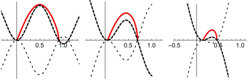
to the quantum-mechanical instanton calculation, where one imagines a particle rolling from a local maximum in the inverted potential, through a minimum, to a position of equal height further along, before returning to its starting point. This is illustrated in Fig. 2 for small, medium and large values of the applied force. The dashed line is the potential V(φ), the dotted line is the inverted potential −V, and the solid line is the (scaled) square root of the potential. The saddle point energy which determines the rate is the area under this curve. This is essentially equivalent to Eq. (23) of ref. 11, but requires no assumptions on the form of the potential. Figure 3 shows H* _as

a function of the applied force (solid curve), along with an approximation (dashed curve) to be discussed below. Since S/4D= H/kBT, the rate can be written as

Figure 2. Potentials for small, medium, and large applied forces (left to right). Dashed line: potential V(φ).

∫

∼ 

  −

   .

φ φ

k T V

rate exp 2 2 ( ) d

(12)

B 0

1

The Arrhenius form derives from the Gaussian white noise, and the explicit damping parameter Γ has cancelled. The

_∫

soliton theory21_{. The analysis above does not require integrability, and shows that this form for the rate survives}

in a driven, dissipative system. This expression is exact as far as the potential is concerned, and holds for any value of F between zero and the Peierls force V0π. It does not require the explicit form of the saddle point configuration,

and hence avoids the need for eigenfunction expansions, or other sophisticated approximation techniques. It can immediately be applied to more complex potentials than the sinusoidal one considered here, e.g. the double-sine form employed in ref. 5 or the computed potentials in refs 15 and 22, and reduces to the results in refs 9, 11 and 23 for appropriate choices of V. It is valid at temperatures kBT< H*, corresponding to the tree-level Feynman

diagrams in quantum field theory. This means it will break down as F→ V0π and H*→ 0. Loop corrections,

cor-responding to larger thermal fluctuations, may be possible if not analytically tractable. For many metals the above rate will be accurate for applied stresses not too close to the Peierls stress, since H* _{at zero F is of order 1 eV}15_.

Fully analytical approximation

Eq. (12) is exact and can be easily evaluated numerically for any F. However, a simple fully analytical expression would be more helpful for use in dislocation dynamics simulations, as well as providing greater insight into the origin of the nonlinearity in the observed rate. This can be obtained by inserting into H[φ] the approximate solu-tion for a sine-Gordon kink-antikink pair separated by R:

φ

π π

= 2 tan e− −µ − + 2 tan e− µ + −_1,

(13)

x R x R

1 ( /2) 1 ( /2)

µ= V π β

( 2 0 2/ ) which leads to

π β µ

= − −µ −

H R( ) 4 2 (1 2 e )V0 R FR, ₍₁₄₎

The three terms correspond to the kink ‘rest energy’, the kink-antikink interaction energy, and the energy gain from the applied bias. Maximizing this expression over R, and writing F=F V/ 0 gives

β π

= 



 − −    _

⁎

H V F F

F

2 8 ln 16 , (15)

KP 20

in agreement with the expression presented in ref. 23. H* _{has been determined numerically using density}

func-tional methods (DFT) for the bcc transition metals15 _{(see in particular Fig. 4 in), and the calculation above is the}

analytical equivalent of the procedure adopted there, where a kink pair ansatz was iterated numerically until con-verged to the extremal configuration. H* _{has also been computed using nudged elastic band simulations for W}22_.

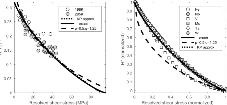
Figure 3. Saddle point energy as a function of the applied force. Left (points): data for edge dislocations

www.nature.com/scientificreports/

Discussion

H_KP is shown as dotted curves in Fig. 3 with HKP⁎ (0)=EKP, the energy of a fully-separated kink pair, set to

0.32 eV. The shape of the curve is in excellent agreement with the numerical results cited above, and the subtle differences may be ascribed to the non-sinusoidal Peierls potentials in real metals. This approximation should hold in the limit F→ 0, yet it captures the exact behaviour remarkably well. Indeed, it only fails when F is within a few per cent of the Peierls force, where the Arrhenius “exp − E/kBT ” form is no longer accurate anyway,

obviat-ing the need for a large F approximation. This is fortuitous, and is due to the sources of inaccuracy compensating each other to some extent. It is now clear how the extreme nonlinearity in the stress dependence of the rate arises: when exponentiated, the second term will become a factor ~FF _{raised to some power. Thus a power series} expan-sion of the rate for small applied forces is not appropriate, and explains the enormous exponents mentioned in the introduction. Especially at low temperatures, the rate resembles a threshold (see Fig. 4 below), and is never linear in the force, however small the force is taken to be. This mathematical effect is not captured by existing nonlinear forms for H* _{such as the elasticity-derived expression H}

0(1 − Fp)q 24,25.

Dislocation velocities are difficult to measure experimentally, and either require in situ straining in the trans-mission electron microscope26_{, where the value of the applied stress is hard to determine, or rely on indirect}

measurements such as slip band growth27_{. The curves in Fig. 3 (left) are fitted to two datasets for edge}

disloca-tions in α-Fe taken from ref. 27 by assuming the dislocation velocity takes the form Aexp(−H*_/k

BT). The fit is

certainly consistent, though caution is required, since the data are taken directly from the log-log plot presented in ref. 27. The values of the Peierls stress and the kink pair energy are somewhat lower than those predicted by DFT15_{, though these DFT calculations were for screw dislocations, and this is not unusual in DFT calculations of}

these quantities in general (see the discussion in ref. 15). The elasticity expression, with p, q= 0.5, 1.25, is shown as dashed lines in Fig. 3. Both forms are consistent with the experimental data, though they require different values for the Peierls potential and kink pair energy. Figure 3 (right) compares the analytical predictions with the enthalpies determined numerically in ref. 15. With the notable exception of vanadium, the curves are in excellent agreement. In this case, the elasticity result cannot be adjusted since the values of the Peierls stress and kink pair energy are known a priori. Given the experimental errors involved, the order-of-magnitude agreement seen here is as good as can be expected.

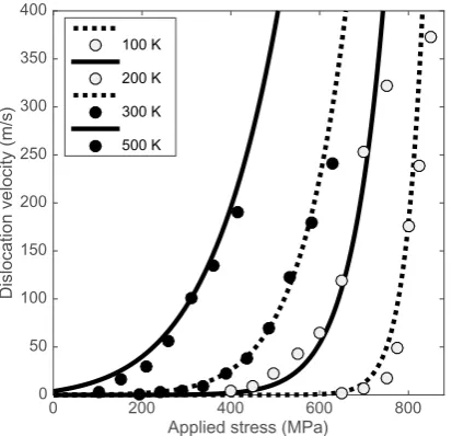
Extensive molecular dynamics simulations of screw dislocations in α-Fe have been performed by Gilbert

et al.25_{. Fitting Aexp(−H}*_/k

BT) to the 300 K data, and changing only the temperature, results in the curves of

Fig. 4. The shapes of the curves, and the temperature-dependence, are in excellent agreement with Fig. 4 of ref. 25. This fit is overly constrained, since as temperature increases, the Peierls potential V0 and string tension β

will change as the elastic moduli of the crystal soften. Also, the prefactor A will be weakly temperature-dependent (though its calculation from quadratic fluctuations implicit in Eq. (6) requires the evaluation of the determinant of a partial differential operator, and is deferred to a future publication). Varying the parameters independently allows a superior fit, though some caution is required. Subtleties arise in the definition of the Peierls stress, e.g. from non-Schmid effects in the applied stress, and changes in the shape of the periodic potential under stress (see ref. 28 and the discussion and references in ref. 25). The functional form of Eq. (15) is clearly appropriate for describing the experimental and numerical results, and for practical purposes such as implementation in discrete dislocation dynamics simulations, a dislocation velocity rule could be obtained by fitting Aexp(−H*_/k

BT) to

what-ever data is available appropriate to the conditions of the simulation.

Figure 4. Points: screw dislocation velocities from MD25_{. Curves:Aexp(−H}*_/k

BT)fitted to the 300 K data



 _ (16)

The analysis also applies to the many other stochastic systems modelled by an elastic string in a periodic potential.

References

1. Kaplan, W. The mechanism of crystal deformation. Science349, 1059–1060 (2015). 2. Hirth, J. & Lothe, J. Theory of dislocations (John Wiley & Sons, 1982).

3. Braun, O. & Kivshar, Y. The Frenkel-Kontorova model: concepts, methods, and applications (Springer Science & Business Media, 2004).

4. Guyer, R. & Miller, M. The sine-Gordon chain. II. Nonequilibrium statistical mechanics. Phys. Rev. A17, 1774 (1978).

5. Fitzgerald, S. & Nguyen-Manh, D. Peierls potential for crowdions in the bcc transition metals. Phys. Rev. Lett. 101, 115504 (2008). 6. Dudarev, S. Coherent motion of interstitial defects in a crystalline material. Phil. Mag. 83, 3577–3597 (2003).

7. Altshuler, T. & Christian, J. The mechanical properties of pure iron tested in compression over the temperature range 2 to 293 degrees K. Phil. Trans. Roy. Soc. London A261, 253–287 (1967).

8. Marchesoni, F. Nucleation of kinks in 1 + 1 dimensions. Phys. Rev. Lett. 73, 2394 (1994).

9. Büttiker, M. & Landauer, R. Nucleation theory of overdamped soliton motion. Phys. Rev. Lett. 43, 1453 (1979).

10. Tarleton, E. & Roberts, S. Dislocation dynamic modelling of the brittle-ductile transition in tungsten. Phil. Mag. 89, 2759–2769 (2009).

11. Dorn, J. E. & Rajnak, S. Nucleation of kink pairs and the Peierls mechanism of plastic deformation. Trans. AIME230, 1052–1064 (1964).

12. Edagawa, K., Suzuki, T. & Takeuchi, S. Motion of a screw dislocation in a two-dimensional peierls potential. Phys. Rev. B55, 6180 (1997).

13. Petukhov, B. & Pokrovskii, V. Quantum and classical motion of dislocations in a Peierls potential relief. Soviet JETP36, 336 (1973). 14. Proville, L., Rodney, D. & Marinica, M.-C. Quantum effect on thermally activated glide of dislocations. Nature Mater. 11, 845–849

(2012).

15. Dezerald, L., Proville, L., Ventelon, L., Willaime, F. & Rodney, D. First-principles prediction of kink-pair activation enthalpy on screw dislocations in bcc transition metals: V, Nb, Ta, Mo, W, and Fe. Phys. Rev. B91, 094105 (2015).

16. Proville, L., Ventelon, L. & Rodney, D. Prediction of the kink-pair formation enthalpy on screw dislocations in α-iron by a line tension model parametrized on empirical potentials and first-principles calculations. Physical Review B87, 144106 (2013). 17. Gurrutxaga-Lerma, B., Balint, D. S., Dini, D., Eakins, D. E. & Sutton, A. P. A dynamic discrete dislocation plasticity method for the

simulation of plastic relaxation under shock loading 469, 20130141 (2013). 18. Wio, H. Path integrals for stochastic processes (World Scientific, 2013).

19. Bray, A., McKane, A. & Newman, T. Path integrals and non-Markov processes. II. escape rates and stationary distributions in the weak-noise limit. Phys. Rev. A41, 657 (1990).

20. Coleman, S. The uses of instantons. In The whys of subnuclear physics, 805–941 (Springer, 1979).

21. Bishop, A., Krumhansl, J. & Trullinger, S. Solitons in condensed matter: a paradigm. Physica D1, 1–44 (1980).

22. Stukowski, A., Cereceda, D., Swinburne, T. D. & Marian, J. Thermally-activated non-schmid glide of screw dislocations in w using atomistically-informed kinetic monte carlo simulations. Int. J. Plasticity65, 108–130 (2015).

23. Hänggi, P., Marchesoni, F. & Sodano, P. Nucleation of thermal sine-gordon solitons: Effect of many-body interactions. Phys. Rev.

Lett. 60, 2563 (1988).

24. Kocks, U., Argon, A. & Ashby, M. Thermodynamics and kinetics of slip. Prog. Mater. Sci. 19, 1–291 (1975).

25. Gilbert, M., Queyreau, S. & Marian, J. Stress and temperature dependence of screw dislocation mobility in α-Fe by molecular dynamics. Phys. Rev. B84, 174103 (2011).

26. Caillard, D. Kinetics of dislocations in pure Fe. part I. in situ straining experiments at room temperature. Acta Mat. 58, 3493–3503 (2010).

27. Turner, A. & Vreeland, T. Jr. The effect of stress and temperature on the velocity of dislocations in pure iron monocrystals. Acta Met.

18, 1225–1235 (1970).

28. Gilbert, M., Schuck, P., Sadigh, B. & Marian, J. Free energy generalization of the Peierls potential in iron. Phys. Rev. Lett. 111, 095502 (2013).

Acknowledgements

This work was partially supported by the UK EPSRC under grant numbers EP/H018921/1 and EP/J014494/1. The author acknowledges useful discussions with Dr Cameron Hall and Prof Sir John Ball FRS, and thanks Dr Lucile Dezerald for providing the numerical data from ref. 15.

Additional Information

Competing financial interests: The authors declare no competing financial interests.

How to cite this article: Fitzgerald, S. P. Kink pair production and dislocation motion. Sci. Rep.6, 39708; doi:

10.1038/srep39708 (2016).

Publisher's note: Springer Nature remains neutral with regard to jurisdictional claims in published maps and

www.nature.com/scientificreports/

This work is licensed under a Creative Commons Attribution 4.0 International License. The images or other third party material in this article are included in the article’s Creative Commons license, unless indicated otherwise in the credit line; if the material is not included under the Creative Commons license, users will need to obtain permission from the license holder to reproduce the material. To view a copy of this license, visit http://creativecommons.org/licenses/by/4.0/