Practical guide to sample size calculations: superiority trials

This is a repository copy of

Practical guide to sample size calculations: superiority trials

.

White Rose Research Online URL for this paper:

http://eprints.whiterose.ac.uk/97114/

Version: Accepted Version

Article:

Flight, L. orcid.org/0000-0002-9569-8290 and Julious, S.A. (2016) Practical guide to

sample size calculations: superiority trials. Pharmaceutical Statistics, 15 (1). pp. 75-79.

ISSN 1539-1604

https://doi.org/10.1002/pst.1718

This is the peer reviewed version of the following article: Flight, L., and Julious, S. A.

(2016) Practical guide to sample size calculations: superiority trials. Pharmaceut. Statist.,

15: 75–79. doi: 10.1002/pst.1718., which has been published in final form at

http://dx.doi.org/10.1002/pst.1718. This article may be used for non-commercial purposes

in accordance with Wiley Terms and Conditions for Self-Archiving

(http://olabout.wiley.com/WileyCDA/Section/id-820227.html).

[email protected] Reuse

Unless indicated otherwise, fulltext items are protected by copyright with all rights reserved. The copyright exception in section 29 of the Copyright, Designs and Patents Act 1988 allows the making of a single copy solely for the purpose of non-commercial research or private study within the limits of fair dealing. The publisher or other rights-holder may allow further reproduction and re-use of this version - refer to the White Rose Research Online record for this item. Where records identify the publisher as the copyright holder, users can verify any specific terms of use on the publisher’s website.

Takedown

If you consider content in White Rose Research Online to be in breach of UK law, please notify us by

Practical guide to sample size calculations:

superiority trials

Laura Flight1

and Steven. A. Julious1

March 24, 2016

Abstract

A sample size justification is a vital part of any investigation. However, estimating the number of participants required to give meaningful results is not always as straightforward. A number of components are required to facilitate a suitable sample size. Practical advice and examples are provided illustrating how to carry out a the calculations by hand and using the app SampSize.

1

Introduction

The introduction paper in this series highlighted the key general components required to estimate the sample size of a clinical trial [1]. This paper provides a practical guide for applying these steps to superiority parallel group clinical trials where the primary endpoint can be assumed to be Normally distributed.

In a superiority trial, the objective is to determine whether there is evidence of a difference in the comparator of interest between the regimens, with reference to the null hypothesis that the regimens are the same.

This paper will go through the steps of a sample size calculation for a supe-riority trial first giving an explanation of supesupe-riority trials and their hypotheses. The formulae for sample size calculations are then given, highlighting how each of the components forms part of the calculation.

Worked examples are used to demonstrate the operational steps in a sample size calculation. The worked examples will use the app SampSize [2] and by-hand solutions to emphasise the ease of calculation. Details of how to obtain the app are provided in Table 1.

Table 1: How to obtain the app SampSize

The SampSize app is available on the Apple App Store to download for free and can be used on iPod Touch, iPad and iPhones. The app is also available on the Android Market. It requires Android version 2.3.3 and above.

2

Components of a Sample Size

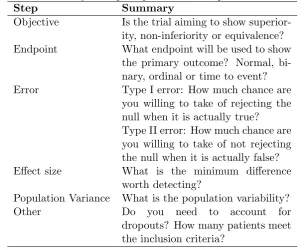
In the introduction to this series, the steps needed for a sample size calculation are identified. Table 2 gives a summary of these points. An important step before carrying out any sample size calculation is being able to complete this table.

Table 2: Summary of steps required for a sample size calculation,

Step Summary

Objective Is the trial aiming to show superior-ity, non-inferiority or equivalence?

Endpoint What endpoint will be used to show

the primary outcome? Normal, bi-nary, ordinal or time to event?

Error Type I error: How much chance are

you willing to take of rejecting the null when it is actually true? Type II error: How much chance are you willing to take of not rejecting the null when it is actually false?

Effect size What is the minimum difference

worth detecting?

Population Variance What is the population variability?

Other Do you need to account for

dropouts? How many patients meet the inclusion criteria?

3

Superiority Clinical Trials

In a superiority trial, the objective is to determine whether there is evidence of a difference in the desired outcome between treatment A and treatment B with mean response A and B, respectively. The hypotheses under consideration are:

H0: The two treatments are not different with respect to the mean response µA=µB.

H1: The two treatments are different with respect to the mean response µA6=µB.

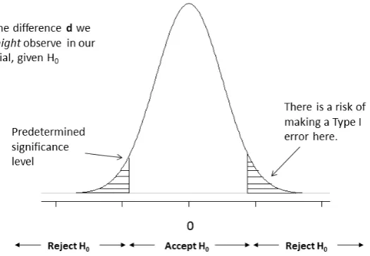
For a superiority trial, the null hypothesis can be rejected if A > B or if

A < B by a statistically significant amount. This results in two chances of making a type I error.

Figure 1: Density plot of superiority trial under the null hypothesis.

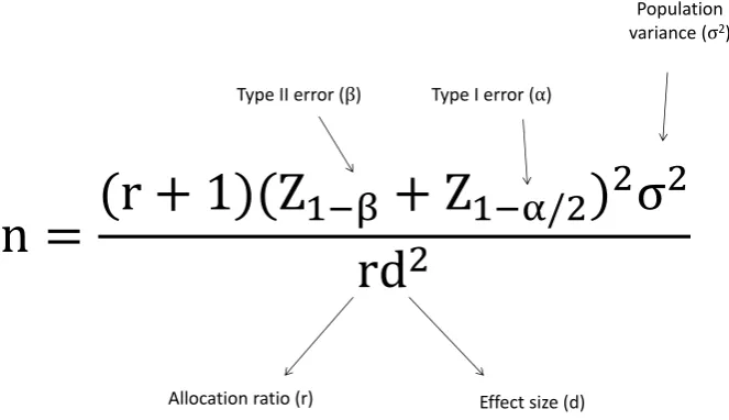
To design a two group trial, the sample size per arm can be estimated [3] from the formula given in Figure 2.

The allocation ratio (r) is such that the number of participants on treatment B isrtimes the number on treatment A, that is, nB =rnA. Note: n=nA+nB

is minimised whenr = 1.

Table 3: Normal deviates for common percentiles. x Z₁−x

0.200 0.842 0.150 1.036 0.100 1.282 0.050 1.645 0.025 1.960 0.010 2.326 0.001 3.090

Table 3 gives common Normal deviates for different percentiles. For example, for β = 0.1, we would have x = 0.1 and Z1_−x = 1.282, while for α = 0.05, we

would havex= 0.025 andZ1_−x= 1.96. These values are useful when calculating

a sample size by-hand.

n

r

Z

_rd

Z

Type II error ( ) Type I error ( )

Population variance ( 2₎

Effect size (d) Allocation ratio (r)

Figure 2: Formula to calculate the sample size for a superiority parallel group trial with Normally distributed endpoint.

analysis, the population variance, σ2

, is usually considered unknown for the analysis, and a sample variance estimate, s2

, is used instead. This is estimated withnA(r+ 1)−2 degrees of freedom. The following formula can be used [3],[4]

1−β=P robt

t1₋α

2−2, nA(r+ 1)−2),

s

rn_Ad2

(r+ 1σ2)

(1)

where Probt(·) is defined as the cumulative density function of a non-central t

distribution, taken from the function in the package SAS (SAS Institute, Inc., Cary, NC, USA). This result gives the power for a given sample size. To estimate a sample size for a given power, we must iterate up the sample sizes until the requisite power is reached. The SampSize app uses the non-centraltdistribution in its calculations.

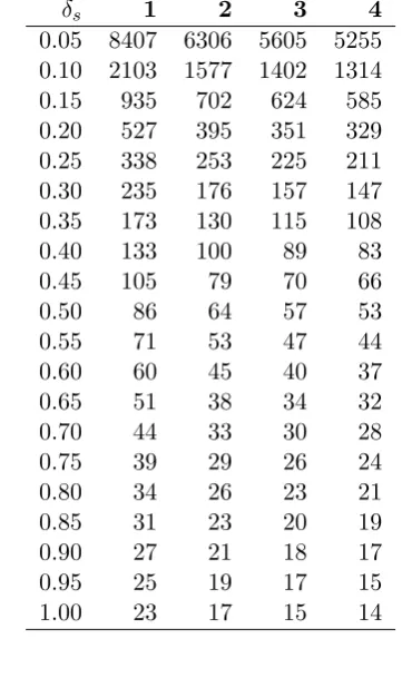
To assist, Table 4 gives sample sizes using (1) for various standardised dif-ferences.

Although the formula in Figure 2 is easier to calculate by-hand, it gives slightly lower sample sizes when compared with (1).

For quick calculations when we have 90% power and a two-sided 5% type I error rate, the following result can be used:

nA=

10.5σ2 d2

(r+ 1)

Table 4: Normal deviates for common percentiles.

δs 1 2 3 4

0.05 8407 6306 5605 5255

0.10 2103 1577 1402 1314

0.15 935 702 624 585

0.20 527 395 351 329

0.25 338 253 225 211

0.30 235 176 157 147

0.35 173 130 115 108

0.40 133 100 89 83

0.45 105 79 70 66

0.50 86 64 57 53

0.55 71 53 47 44

0.60 60 45 40 37

0.65 51 38 34 32

0.70 44 33 30 28

0.75 39 29 26 24

0.80 34 26 23 21

0.85 31 23 20 19

0.90 27 21 18 17

0.95 25 19 17 15

1.00 23 17 15 14

or forr= 1:

n_A= 21σ

2

d2 (3)

4

Cactus Example

In the CACTUS clinical trial [5], participants suffering from long-standing apha-sia post stroke are to be randomised to one of three arms:

1. usual care,

2. self-managed computerised speech and language therapy in addition to usual care and

3. attention control in addition to usual care.

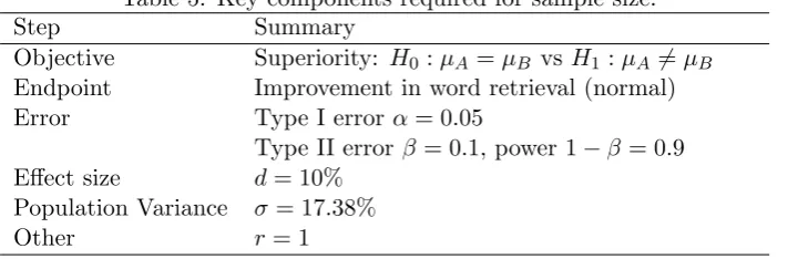
The primary objective of the trial is to compare usual care with self-managed computerised therapy. The primary outcome of interest is the change in the num-ber of words named correctly at 6 months. The minimal clinically meaningful difference is improvement in word retrieval of 10%. Based on a pilot study [5], the population standard deviation is assumed to be 17.38%. The dropout rate applied is 15% (95% confidence interval (CI), 5-32%).

Table 5: Key components required for sample size.

Step Summary

Objective Superiority: H0 :µ_A=µ_B vs H1 :µ_A6=µ_B

Endpoint Improvement in word retrieval (normal)

Error Type I error α= 0.05

Type II errorβ = 0.1, power 1−β = 0.9

Effect size d= 10%

Population Variance σ = 17.38%

Other r = 1

After identifying these key points summarised in Table 5, it is possible to plug the values into the formula in Figure 2. This gives

n_A= (1 + 1)(Z1−0.1+Z1−0.05/2)

2

(17.382

)

1×102 (4)

Using the common percentiles from Table III, the sample size is 64 for each group. To apply the 15% dropout rate, we divide by the completion rate (100%-15%= 85%). This suggests that 76 participants are needed in each arm of the trial.

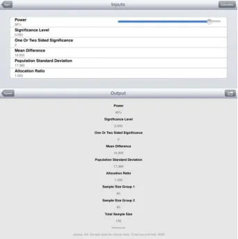
The app SampSize can also be used for the calculation. To use the app, you need to select options: Superiority, Parallel Group, Normal and Calculate Sample Size. You then get to the top screen as given Figure 3.

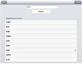
Each component of the sample size calculation can be entered into the app. For ease, the app provides a list of suggested entries you can select from. For example (Figure 4), if you select Significance Level, the next screen gives the options 0.001, 0.01, 0.02, 0.025, 0.03, 0.04, 0.05, 0.075 and 0.10 (sic). Alterna-tively, you can select the Custom option where it is possible to enter a value for the significance level manually.

SampSize gives a sample size of 65 per group. Applying the 15% dropout rate, a total of 154 participants are required to achieve 90% power. The difference in the two sample size estimates arises because SampSize uses a non-central t

distribution to estimate the sample size.

To use the sample size table, we first need to estimate the standardised difference,

δ= d

σ =

10

17.38 = 0.575 (5)

Unfortunately, when using the tables, the standardised differences increase in increments of 0.05. As a result, there is no entry in Table 4 for this standardised difference. Standardised differences of δ = 0.55 and δ = 0.60 give sample sizes of 71 and 60, respectively. A sample size of 71 is a conservative estimate, which we would need to amend using SampSize or other calculations.

to recruit 77 patients per arm. However, once the trial has begun, we experience a much higher dropout rate of 32%, and our evaluable sample size decreases to 53. We can use the app to estimate the power of our study with this smaller sample size.

As before, select a Superiority, Parallel Group trial with a Normal endpoint, but now rather than choosing to calculate a sample size, select to calculate power. With the same inputs as before but with a sample size of 53, the power is estimated to be 83%. Although this is still an acceptable power, it is much less than the proposed 90% power.

Figure 3: Screenshot of SampSize app custom settings for a sample size calcula-tion.

Figure 4: Screenshot of SampSize app for CACTUS worked example.

5

Summary

This paper has illustrated how to calculate sample sizes for superiority trials where the data are assumed to be Normally distributed. It builds on the steps identified in the first paper of the series for sample size estimation. The paper gives formulae for sample size estimation from quick easy-to-use results to more complicated calculations that require iteration to find a solution. To assist in the calculations, sample size tables and calculations using an app SampSize are described.

The subsequent papers in the series applies these ideas to non-inferiority and equivalence [6].

6

Acknowledgements

References

[1] Flight L, Julious SA. Practical guide to sample size calculations: an intro-duction.Pharmaceutical Statistics.

[2] epiGenesys. A University of Sheffield company. Available at https://www.epigenesys.org.uk/portfolio/sampsize//. (accessed 07.07.2015).

[3] Julious SA. Sample Sizes for Clinical Trials. Chapman and Hall: Boca Ra-ton, Florida, 2009.

[4] Julious SA. Tutorial in Biostatistics: sample sizes for clinical trials with Normal data.Statistics in Medicine _{2004; 23:19211986.}

[5] Palmer R, Enderby P, Cooper C, Latimer N, Julious S, Paterson G, Dimairo M, Dixon S, Mortley J, Hilton R, Delaney A, Hughes H. Computer therapy compared with usual care for people with long-standing aphasia poststroke: a pilot randomized controlled trial.Stroke _{2012; 43:19041911.}