This is a repository copy of
Simulation or cohort models? : Continuous time simulation and
discretized Markov models to estimate cost-effectiveness
.
White Rose Research Online URL for this paper:
http://eprints.whiterose.ac.uk/75218/
Monograph:
Soares, M. orcid.org/0000-0003-1579-8513 and Canto e Castro, L. (2010) Simulation or
cohort models? : Continuous time simulation and discretized Markov models to estimate
cost-effectiveness. Working Paper. CHE Research Paper . Centre for Health Economics
[email protected] https://eprints.whiterose.ac.uk/
Reuse
Items deposited in White Rose Research Online are protected by copyright, with all rights reserved unless indicated otherwise. They may be downloaded and/or printed for private study, or other acts as permitted by national copyright laws. The publisher or other rights holders may allow further reproduction and re-use of the full text version. This is indicated by the licence information on the White Rose Research Online record for the item.
Takedown
If you consider content in White Rose Research Online to be in breach of UK law, please notify us by
Simulation or Cohort Models?
Continuous Time Simulation and
Discretized Markov Models to
Estimate Cost-Effectiveness
Simulation or cohort models?
Continuous time simulation and discretized
Markov models to estimate cost-effectiveness
Marta O Soares
1L Canto e Castro
21
Centre for Health Economics, University of York, UK
2
Department of Statistics and Operations Research, Faculty of Sciences,
University of Lisbon, Portugal
Background
CHE Discussion Papers (DPs) began publication in 1983 as a means of making current research material more widely available to health economists and other potential users. So as to speed up the dissemination process, papers were originally published by CHE and distributed by post to a worldwide readership.
The CHE Research Paper series takes over that function and provides access to current research output via web-based publication, although hard copy will continue to be available (but subject to charge).
Disclaimer
Papers published in the CHE Research Paper (RP) series are intended as a contribution to current research. Work and ideas reported in RPs may not always represent the final position and as such may sometimes need to be treated as work in progress. The material and views expressed in RPs are solely those of the authors and should not be interpreted as representing the collective views of CHE research staff or their research funders.
Further copies
Copies of this paper are freely available to download from the CHE website
www.york.ac.uk/inst/che/pubs. Access to downloaded material is provided on the understanding that it is intended for personal use. Copies of downloaded papers may be distributed to third-parties subject to the proviso that the CHE publication source is properly acknowledged and that such distribution is not subject to any payment.
Printed copies are available on request at a charge of £5.00 per copy. Please contact the CHE Publications Office, email [email protected], telephone 01904 321458 for further details.
Centre for Health Economics Alcuin College
University of York York, UK
www.york.ac.uk/inst/che
Abstract
1.
Introduction
Decisions to fund and use health care technologies are increasingly informed by cost-effectiveness analysis (CEA). The goal of CEA is to identify the 'preferred' option from a choice of health technologies to fund from available resources. This goal is achieved through measurement of the expected marginal costs and effects associated with the displacement of a health technology by a new one.1 The outcomes of the analysis are the incremental cost-effectiveness ratio (ICER) — the additional cost per extra unit of effect from the more effective option2 — or the net benefit (NB) statistic. To make a decision regarding which treatment option is cost effective, a decision rule is then applied.3 Given that there is uncertainty in the joint distribution of incremental costs and effects, the decision itself is uncertain. An assessment of this uncertainty is a key requirement of economic evaluation for decision making4and can be used to establish the value of further research.5
Agencies such as the UK National Institute for Health and Clinical Excellence (NICE) require that all relevant available evidence should be considered to inform decision making. In the presence of multiple sources of information, this involves bringing together and synthesising evidence appropriately in terms of input data, e.g. mortality, relative risks or utility weights.6,7 Based on these input parameters, the expected cost and effect is calculated for each alternative treatment option by weighting the likelihood of disease consequences by their cost. The mathematical relations between inputs from different sources and outputs are brought together by a decision analytic model (DAM).
The design and structure of DAMs should characterise the consequences of alternative treatment options in a way that is appropriate to the decision problem. DAMs can be based on cohort (aggregated) models. These are defined here as having a closed form solution, that is the expected costs and effects based on the average patient experience are evaluated algebraically, although there are other definitions. The majority of DAMs applied in the context of chronic or long-term diseases use aggregated state transition models8, and assume independence of individuals within the model.9 These models are defined by a set of mutually exclusive health states and the movement between these states through time represents possible patient disease (or health) pathways to which costs and effects can be assigned. When discrete time models, such as discrete time Markov models10,11, are defined, the probability of occupying a given state is assessed over a series of discrete and constant time periods, known as cycles. An important characteristic of Markov models is that future development of the process is not dependent on the history of the process, just on the present (Markov property). Although this property can simplify the use of such models, it is often unrealistic. To circumvent dependency on time spent in a specific state a set of tunnel states can be implemented in a Markov framework10or a semi-Markov framework12,13may be used.
However, it is important to note that time has a continuous nature. When the decision problem relates to a chronic disease, the phenomena one wishes to evaluate can be described as a series of events occurring through time; thus the theoretical model used to mimic such phenomena should ideally represent time as a continuous measure. Whilst continuous time models can be employed, they rarely are in practice since closed form solutions for the expected time spent in states may not exist when a continuous time formulation of a state transition model is used, such as for semi-Markov models.14 Furthermore, even when such closed form solutions do exist, these can be mathematically demanding if, for example, the transition rates are not constant through time.15,16 To overcome this issue a discrete time approximation (discretized cohort models) is often applied to continuous time phenomena. Whilst in continuous time models individuals can transit at any time to the absorbing state, in discretized models individuals can only transit in discrete time periods. An important issue when using discretization, or any numerical method, is that the shorter the discretization step (or cycle length) the better the approximation to continuous time model outcomes.17 Although discrete time models are frequently applied in the evaluation of cost-effectiveness, the outcomes of such models are seldom regarded as approximations (to continuous time). As a result determinants of bias such as the cycle length are disregarded.
2 CHE Research Paper 56
Whichever DAM design is used, the parameters are uncertain since they are estimated directly from sampled data or from evidence synthesis procedures. The decision to adopt the new intervention will also be uncertain. It then matters to evaluate how confident we are that the intervention is cost-effective.19 The propagation of the joint uncertainty on model inputs to model outputs is called probabilistic sensitivity analysis (PSA). This process is usually conducted by simulation: in a frequentist framework a second order Monte Carlo method is used, while in the Bayesian framework the uncertainty is represented directly by the posterior distribution of the ICER or NB.20,21 PSA is relatively straightforward in cohort models. However, for individual stochastic simulation models the full assessment decision uncertainty using PSA may not viable as two levels of simulation are required: for each realization of the set of uncertain parameters (as part of PSA), a Monte Carlo simulation is required to evaluate the expected values of outcomes.22Some authors disregard the use of these models when it compromises the evaluation of second order uncertainty.23
While the distinction between discrete time and continuous time is mathematically clear-cut, it is unclear from the existing literature how the use of a discrete time approximation to continuous time phenomena can affect the evaluation of cost-effectiveness, and hence the decision recommendation for the underlying policy problem. Alternatively, continuous time models evaluated by Monte Carlo simulation can be used to estimate the same outcomes. These return imprecise estimates and may place heavy demands upon computational resources, especially when a second simulation procedure for PSA is required. Although simulation and discrete model outcomes were previously compared24, the continuous nature of time was ignored and both models were built assuming discrete time. Additionally, published guidance on model design25does not explicitly consider discrete time models as approximations.
This work intends to draw recommendations on the use of discretized cohort model and simulation approaches, when these constitute alternative model designs in cost-effectiveness analysis aiming at evaluating a decision problem characterised by continuous time evolvement. To pursue this in an intuitive way, a hypothetical decision problem will be defined where an exact solution for outcomes exists. This obliges the choice of a simple example, maybe unrepresentative of many DAMs as applied in current practice, but that demonstrates theoretical results obtainable with any other model.
2.
Methods
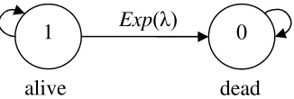
[image:10.595.219.382.159.214.2]In order to compare the cost-effectiveness estimates from stochastic simulation and cohort models, a true process representing reality is defined with two health states: alive and dead (Figure 1).
Figure 1: Two state model including one absorbent state (dead state)
An individual initiates the chain alive and may remain alive or die over time; that is, transit to state 0 (dead). Death is represented by an absorbent state from which there is zero probability of exiting. The transitions to death occur at a constant rate, . Consequently, time to event follows an exponential distribution, Exp().
2.1. Life expectancy
The above process can be perfectly described by a continuous time homogeneous Markov chain, where the probability of transiting between states is not dependent on time itself, but is dependent on the length of the time interval, or cycle, considered. For a continuous time two state process, the expected time until absorption, or life expectancy
E T
, can be defined as the expected value of theunderlying distribution assumed for the time to transition. If the underlying distribution is exponential,
E T
is given by
1
E T =
(1)
where
is the parameter of the exponential distribution.Although approximations are unnecessary in the current example, the existence of the closed form solution of life expectancy allows evaluating bias associated with the estimates obtained through a discretized model and a continuous time simulation model.
Discretized Markov models
Numerical solutions, or quadrature methods, can be used to solve complex integrals and in the current context this involves evaluating the model in discrete time. In the Appendix, the general case for a discrete time homogeneous Markov model is detailed. The calculation of life expectancy is based on the probability of transiting in one cycle, which is naturally defined by the probability of a transition occurring in the same period of time in the corresponding continuous time process.26 The discretized transition probability of dying,
P
10, for the two state model is1
e
HT(tn1)HT( )tn
,where HT(tn) represents the cumulative hazard function evaluated at time tn for the random variable (r.v.)
T
representing time to death. WhenT assumes an exponential distribution the discretized one step transition probability can be simplified to10
P
1
e
l (2)where
l
is the cycle length. The unrestricted life expectancy, denoted here byE T
1
, estimated bya two state discretized process can be defined by
1
Exp
( )
0
4 CHE Research Paper 56
110
1
E T
l
P
, (3)where the expected number of transitions until absorption is multiplied by the cycle length,
l
. The accuracy of using a discretized process to evaluate continuous time outcomes depends on the discretization of the continuous distribution into cycle lengths. Asl
tends to zero the discretized Markov chain converges to the continuous one.CEA are conducted often assuming a finite time horizon, K, for outcome evaluation. A restricted life
expectancy estimate,
E
2
T
, for the model depicted in Figure 1 can be assessed through theunconditional probabilities (see Appendix 1), as given by:
2 10
0
E
T =
K n
n
P
l
, (4)Continuous time Markov models evaluated through Monte Carlo simulation
Monte Carlo methods rely on stochastic simulation, that is, in the reproduction of values from a probability distribution. A sample value of time until the occurrence of a discrete event (here death) is drawn from a predefined distribution. Costs and utilities are assigned to the time spent in the health state (here alive). The procedure is repeated
N
times and the sample average of the costs and benefits returns the best estimate for the expected costs and benefits associated with the interventionunder evaluation. The estimates obtained with Monte Carlo simulation will be denoted by
E T
ˆ
3
. Adetailed description of this procedure is shown in the Appendix. The validity of the Monte Carlo estimates is dependent on the evaluation of convergence and on the precision associated with the estimates. Precision relies on the size of the simulated sample.
2.2. Costs and QALYs
Quality-adjusted life weights and unit costs are assigned to the time spent in states other than death. If unit costs and utility weights are assumed non-stochastic, i.e. have no uncertainty, it is possible to obtain a closed form solution for expected total costs and expected quality-adjusted life years (QALYs). The expected total costs,
E C
, and expected total QALYs,E U
, are given by:
E C =E T
c
andE U =
E T
u
(5)3.
Discretized versus simulation Markov models.
An evaluation of
cost-effectiveness
The variable representing lifetime or time until absorption,
T
, is assumed to follow an exponential distribution with a rate parameter of
. If
0.1
the expected time to absorption of a continuous time Markov chain (Equation 1) is given by the expected value of the exponential distribution, i.e. 10 time units (defined as years in this example).3.1.
Estimates of life expectancy
To evaluate the influence of the discretization step, unrestricted expected lifetimes (Equation 3) were obtained through the discretized homogeneous Markov model for different cycle lengths. In Table 1
[image:12.595.99.498.373.472.2]and Figure 2 the life expectancy unrestricted estimates are reported for cycle lengths defined by
1
2
l wherel
is an integer varying between 0 and 6. These estimates were obtained by evaluating a discrete time Markov process where the one step transition probabilities were estimated (Equation 2) as function of the theoretical continuous time rate and the cycle length. As an example, the transition probability between the states alive and dead assumes the value of 0.0952 for a cycle length of one year. The application of discretized models to assess continuous time phenomena will return approximate estimates, and the difference between the estimate or approximate value and the true value was assessed as an empirical measure of bias.Table 1: Discretized Markov model evaluations of life expectancy, conditional on cycle length. Estimates obtained from unrestricted and restricted solutions of the discretized process.
Discrete time unrestricted
Discrete time
restricted (time horizon = 20 years)
Cycle length
Estimate Bias Cycle
length
Estimate Bias
1 10.51 0.508 1 9.22 -0.78 0.5 10.25 0.252 0.5 8.93 -1.07 0.25 10.13 0.126 0.25 8.79 -1.21 0.125 10.06 0.063 0.125 8.72 -1.28 0.015625 10.01 0.008 0. 015625 8.65 -1.35
Unrestricted life expectancy (
E T
1
) evaluated through the discretized model is always bigger thanor equal to the theoretical life expectancy (10 years) (unrestricted case in Table 1, and Figure 2). Hence the associated bias is always positive. As one shortens the cycle length, the discretized solution approaches the continuous time process solution. Note that using a 1 year cycle length overestimates time until absorption by about 0.5 years.
Cycle length L if e e x p e c ta n c y
0.0 0.2 0.4 0.6 0.8 1.0
1 0 .0 0 1 0 .2 5 1 0 .5 0 discretized model theoretical
[image:12.595.161.419.583.718.2]6 CHE Research Paper 56
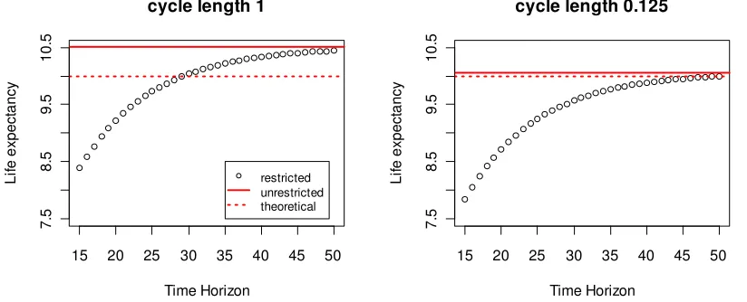
When the discrete process is evaluated in a finite time horizon, a “restricted” estimate of the expected outcomes is obtained
(
E T
2
,
(Equation 4). The restricted estimate of life expectancy is always lessthan or equal to the unrestricted one. Figure 3 shows the life expectancy obtained through the application of distinct restriction points, or time horizons, for cycle lengths of 1 and 0.125.
15 20 25 30 35 40 45 50
7 .5 8 .5 9 .5 1 0 .5
cycle length 1
Time Horizon L if e e x p e c ta n c y restricted unrestricted theoretical
15 20 25 30 35 40 45 50
7 .5 8 .5 9 .5 1 0 .5
cycle length 0.125
Time Horizon L if e e x p e c ta n c y
Figure 3: Theoretical life expectancy calculated from the discretized model with 1 year (plot on the left) and 0.125 years of cycle length (plot on the right). The full line represents the expected time to absorption of the unrestricted discretized time process and the dotted line the expected time to
absorption of the true, continuous time phenomena.
[image:13.595.87.499.144.311.2]As the time frame of restriction gets larger, the life expectancy approaches the unrestricted one. Hence there is decreasing bias when the time horizon of analysis tends to infinity and the cycle length approaches zero.
[image:13.595.199.396.554.650.2]Table 2 presents the results of the model when the life expectancy is estimated through Monte Carlo simulation. With 100,000 Monte Carlo simulations, an estimate of 10 years of life expectancy is obtained. The standard error associated with this estimate is 0.032 (Table 2), and the convergence diagnostic plot is shown in Figure 4. Methods based on stochastic simulation are inheritably approximate as the simulated sample will never be an exact reproduction of the true distribution.
Table 2: Life expectancy estimates of a continuous time Markov model evaluated through Monte Carlo simulation.
Continuous time
N simulations
E
ˆ
3
T
SE(E
ˆ
3
T
)100 9.85 0.856 1000 9.95 0.318 10000 10.03 0.099 100000 10.00 0.032
[image:13.595.201.395.555.651.2]o o o o o o o o o o o oo oo oo oooooooo o o o o o o oooooooooooooo
o
ooooooooooooooooooooooooooooooooooooooooooooooooooooooooooooooooooooooooooooooooooooooooooooooooooooooooooooooooooooooooooooooooooooooooooooooooooooooooooooooooooooooooooooooooooooooooooooooooooooooooooooooooooooooooooooooooooooooooooooooooooooooooooooooooooooooooooooooooooooooooooooooooooooooooooooooooooooooooooooooooooooooooooooooooooooooooooooooooooooooooooooooooooooooooooooooooooooooooooooooooooooooooooooooooooooooooooooooooooooooooooooooooooooooooooooooooooooooooooooooooooooooooooooooooooooooooooooooooooooooooooooooooooooooooooooooooooooooooooooooooooooooooooooooooooooooooooooooooooooooooooooooooooooooooooooooooooooooooooooooooooooooooooooooooooooooooooooooooooooooooooooooooooooooooooooooooooooooooooooooooooooooooooooooooooooooooooooooooooooooooooooooooooooooooooooooooooooooooooooooooooooooooooooooooooooooooooooooooooooooooooooooooooooooooooooooooooooooooooooooooooooooooooooooooooooooooooooooooooooooooooooooooooooooooooooooooooooooo
Sample size A v e ra g e L E e s ti m a te o o o oo oo oo oooooooo o oooooooooooo
o
oooooooooooooooooooooooooooooooooooooooooooooooooooooooooooooooooooooooooooooooooooooooooooooooooooooooooooooooooooooooooooooooooooooooooooooooooooooooooooooooooooooooooooooooooooooooooooooooooooooooooooooooooooooooooooooooooooooooooooooooooooooooooooooooooooooooooooooooooooooooooooooooooooooooooooooooooooooooooooooooooooooooooooooooooo oooooooooooooooooooooooooooooooooooooooooooooooooooooooooooooooooooooooooooooooooooooooooooooooooooooooooooooooooooooooooooooooooooooooooooooooooooooooooooooooooooooooooooooooooooooooooooooooooooooooooooooooooooooooooooooooooooooooooooooooooooooooooooooooooooooooooooooooooooooooooooooooooooooooooooooooooooooooooooooooooooooooooooooooooooooooooooooooooooooooooooooooooooooooooooooooooooooooooooooooooooooooooooooooooooooooooooooooooooooooooooooooooooooooooooooooooooooooooooooooooooooooooooooooooooooooooooooooooooooooooooooooooooooooooooooooooooooooooooooooooooooooooooooooooooooooooooooooooooooooooooooooooooooooooooo o o o o o o o o o o o o o o o o o o o o o o o o o o o o o o o o o o o o o o o o o o o o o o o o o o o o o o o o o o o o o o o o o o o o o o o o o o o o o o o o o o o o o o o o o o o o o o o o o o o o o o o o o o o o o o o o o o o o o o o o o o o o o o o ooo o o o o o o oooo oooooooooo o o o o o o ooo o ooooooooo
oo oooooooooooooooooooooooooooooooooooooooooooooooooooooooooooooooooooooooooo
oooooooooooooooooooooooooooooooooooooooooooooooooooooooooooooooooooooooooooooooooooooooooooooooooooooooooooooooooooooooooooooooooooooooooooooooooooo o
ooooooooooooooooooooooooooooooooooooooooooooooooooooooooooooooooooooooooooooooooooooooooooooooooooooooooooooooooooooooooooooooooooooooooooooooooooooooooooooooooooooooooooooooooooooooooooooooooooooooooooooooooooooooooooooooooooooooooooooooooooooooooooooooooooooooooooooooooooooooooooooooooooooooooooooooooooooooooooooooooooooooooooooooooooooooooooooooooooooooooooooooooooooooooooooooooooooooooooooooooooooooooooooooooooooooooooooooooooooooooooooooooooooooooooooooooooooooooooooooooooooooooooooooooooooooooooooooooooooooooooooooooooooooooooooooooooooooooooooooooooooooooooooooooooooooooooooooooooooooooooooooooooooooooooooooooooooooooooooooooooooooooooooooooooooooooooooooooooooooooooooooooooooooo o oooooooooooooooooooooooooooooooo
0 20 000 40 000 60 000 80 000 100 000
[image:14.595.159.424.108.227.2]9 1 0 1 1 o o point estimate confidence interval
Figure 4: Convergence diagnostic plot: life expectancy estimates (black) and normal based confidence intervals (grey), obtained through Monte Carlo simulation of a continuous time model considering
varying sample sizes (index).
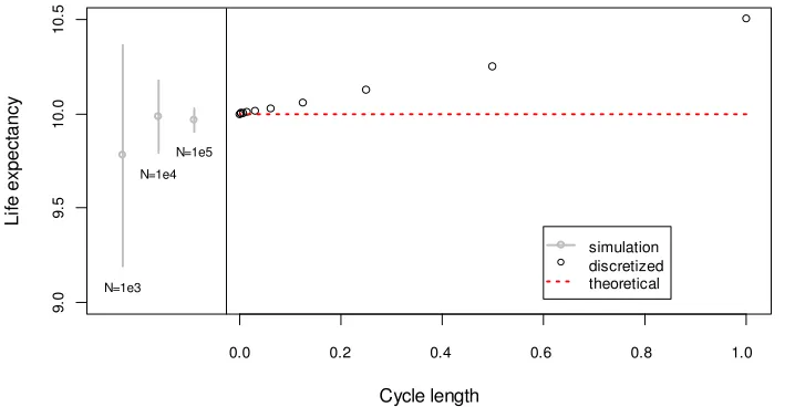
The time to absorption or life expectancy estimates obtained with both the discretized (unrestricted estimate) and simulation Markov models are represented in Figure 5. The black hollow points represent the unrestricted life expectancy estimates from a discretized process, conditional on distinct values of the cycle length, as seen in Figure 2. The life expectancy estimate obtained through Monte Carlo simulation (for different sample sizes) and the associated 95% confidence interval (normal approximation) is represented in grey.
Cycle length L if e e x p e c ta n c y
0.0 0.2 0.4 0.6 0.8 1.0
9 .0 9 .5 1 0 .0 1 0 .5 N=1e5 N=1e4 N=1e3 simulation discretized theoretical
Figure 5: Life expectancy estimates obtained through the discretized and continuous time simulation models. Discretized Markov chain results shown in black for distinct cycle lengths (in x axis). The point
estimate and confidence intervals for the simulation procedure are depicted in grey for Monte Carlo sample sizes of 1 000, 10 000 and 100 000. The dashed horizontal line represents the theoretical life
expectancy.
The approximations obtained through the unrestricted evaluation of the discretized process are closed form solutions, that is, non-stochastic. Additionally, if one reduces the discretization step (cycle length), the estimates obtained through the discretized process tend to be unbiased. On the contrary, the precision of the Monte Carlo procedure is dependent on the sample size.
3.2.
Incremental cost, effects, and cost-effectiveness outcomes.
[image:14.595.114.473.386.570.2]8 CHE Research Paper 56
20% relative to standard treatment. The use of the new treatment, when displacing the standard one, is expected to bring gains of 2.5 years of life expectancy per patient. In addition, it was assumed that patients undergoing treatment with the standard alternative incur £5 000 per year when alive and are assigned a utility weight of 0.8 per year. The new treatment costs an additional £2 250 per year lived, and does not improve patient health related quality of life.
Adopting the new technology over the comparator gives an exact incremental gain in life expectancy of 2.5 years. This equates to 2 additional QALYs gained, but at an additional cost of £40 625 (exact solution). The true expected ICER related to the adoption of the new health technology is therefore £20 312.5 per QALY gained.
[image:15.595.49.550.273.426.2]Using the discretized model to evaluate the incremental cost, effect and cost-effectiveness outcome returns the results shown in Table 3.
Table 3: Incremental costs, effectiveness (LE, life expectancy, and QALYs) and cost-effectiveness outcomes estimated through the discretized Markov model, for distinct cycle lengths. Unrestricted and
restricted estimates.
Unrestricted estimates Restricted estimates (time horizon = 30 years)
Incremental outcomes
Cost-effectiveness Incremental outcomes Cost-effectiveness
Cycle length LE (years) QALYs (years) Costs (£) ICER (£/QALY) bias LE (years) QALYs (years) Costs (£) ICER (£/QALY) bias
1.0000 2.4983 1.9987 39507 19767 -546 1.8825 1.5060 33977 22561 2248 0.5000 2.4996 1.9997 40064 20035 -277 1.8737 1.4989 34434 22972 2660 0.2500 2.4999 1.9999 40344 20173 -140 1.8689 1.4951 34663 23184 2872 0.1250 2.5000 2.0000 40484 20242 -70 1.8664 1.4931 34778 23292 2979 0.0156 2.5000 2.0000 40607 20304 -9 1.8642 1.4914 34879 23387 3074
Incremental outcomes evaluated through the unrestricted discretized model appear to be less prone to bias than non-incremental estimates, naturally due to their relative nature. QALY gains estimated by a discretized model considering a cycle length of one year are estimated to be 1.9987 when the true expected gains are 2 QALYs, returning an absolute bias of 0.013 QALYs. For the current example, although gains in effectiveness are overestimated when long cycle lengths are considered, both the incremental costs and ICER are underestimated. When restricting the time horizon to 30 years, the ICER is overestimated and reducing the cycle length does not guarantee a better approximation.
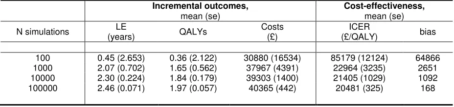
Monte Carlo estimates of incremental outcomes are theoretically unbiased when convergence is achieved. With a sample size of only 100 simulations, the estimate of the ICER is as large as £85 179 per QALY with a bias of £64 866. Increasing the number of simulations to 100 000 (using distinct seeds for the random number generator each time a sample size is set), results in a bias as low as £168/QALY (Table 4).
Table 4: Incremental cost, effectiveness (LE, life expectancy, and QALYs) and cost-effectiveness estimates, obtained from continuous time model through Monte Carlo simulation for varying Monte Carlo
sample sizes.
Incremental outcomes,
mean (se)
Cost-effectiveness,
mean (se) N simulations LE
(years) QALYs
Costs (£)
ICER
(£/QALY) bias
[image:15.595.66.530.654.764.2]10 CHE Research Paper 56
4.
Discussion
In published health technology assessment studies the choice of model design is rarely adequately justified. The current work addresses this issue noting that ideally DAMs should represent phenomena occurring in continuous time. Often, continuous time models do not return a closed form solution (e.g. semi-Markov models) or these solutions are mathematically burdensome to derive (e.g. Markov models with complex structures). In such cases, discretized models are often evaluated but with little regard to the associated bias which is dependent on the cycle length (or discretization step). Alternatively, continuous time models evaluated by Monte Carlo simulation can be used but these simulation methods return imprecise estimates, where their precision is dependent on the dimension of the simulated sample.
We have used an example for which exact solutions are available. The example, even simple, intends to demonstrate how important it is to acknowledge and consider determinants of bias in the estimation. We have shown that, when alternative models can be applied to represent a continuous time phenomena, it is preferable to implement a cohort discretized model than a simulation model, as the bias from the first can be assessed by reducing the cycle length, whilst the second is inherently stochastic. And these recommendations are directly applicable to any other (more complex) situation.
Although discretized cohort models can produce valuable estimates of cost and effectiveness outcomes, the evaluation of cycle length has received little attention when applied in cost-effectiveness assessment. The cycle length is the basis of use of numerical approximations and its importance is recognised in specialized literature.17 As these cohort models constitute approximate solutions, the definition of cycle length cannot be solely based on data availability or clinical feasibility25, but should be varied to examine small changes in outcomes.
In the current work, the use of continuity corrections such as the half-cycle correction was not evaluated. Neither was the use of methods to accelerate convergence in numerical analysis (e.g. Richardson’s extrapolation, see 27) where the necessary accuracy is achieved without needing very short cycle lengths. Although the implementation of these measures is intended to reduce the bias of discretizing the process, the assessment of their effectiveness will always be dependent on reducing the cycle length until no significant changes in the decision are produced.
When designing an economic evaluation study, we argue that the analyst cannot ignore the use of discretized cohort models unless all the conventionally defined models are deemed inappropriate to represent the decision problem context. In this case, simulation modelling should be considered as its use will be translated into gains in accuracy.28
Simulation models benefit from the lack of structural restrictions. This characteristic accounts for the flexibility of such models, but it is the main reason for the lack of transparency attributed to simulation models.29While cohort models represent a well defined relation between parameters and listing the input estimates can be enough to replicate the analysis, simulation models can often only be reproduced when the programmed code is made available. Frequently in the health technology assessment literature simulation models are reported incompletely, their use is not adequately justified, and these are often set up with structural features trivial to the appraisal. The use, design and reporting of simulation models could be greatly improved if more guidance is made available. To overcome the difficulty of conducting PSA alongside simulation models, efficient programming30and emulators31,32 must be further explored. Also, it is important to evaluate convergence and precision of the model estimates, and these could be used to define the Monte Carlo sample size and increase efficiency.
5.
References
1. Garber A and Phelps C. 1997. Economic foundations of cost-effectiveness analysis. Journal of Health Economics16:1–31.
2. Stinnett AA, Paltiel AD. 1997. Estimating CE ratios under second-order uncertainty: the mean ratio versus the ratio of means.Medical Decision Making17(4): 483–489.
3. Johannesson M, Weinstein MC. 1993. On the decision rules of cost-effectiveness analysis, Journal of Health Economics.12(4): 459-467.
4. Claxton K, Sculpher M, McCabe C, Briggs A, Akehurst R, Buxton M, Brazier J, O’Hagan T. 2005. Probabilistic sensitivity analysis for nice technology assessment not an optional extra. Health Economics14: 339–347.
5. Claxton, K. 1999. The irrelevance of inference: a decision making approach to the stochastic evaluation of heath care technologies.Journal of Health Economics18:341–364.
6. Gold M, Siegel J, Russell L, Weinstein M. 1996.Cost-effectiveness in health and medicine(First ed.). Oxford University Press.
7. Drummond M, O’Brien B, Stoddard G, Torrance G. 2001.Methods for the economic evaluation of health care programmes. Oxford University Press: Oxford
8. Karlin S, Taylor H. 1981. A second course in stochastic processes (2nd ed.). San Diego, California: Academic Press.
9. Barton P, Bryan S, Robinson S. 2004. Modelling in the economic evaluation of health care: selecting the appropriate approach.Journal of Health Services Research and Policy 9: 110–118. 10. Sonnenberg FA, Beck JR. 1993. Markov models in medical decision making: a practical guide.
Medical Decision Making.13(4): 322–338.
11. Briggs A and Sculpher M. 1998. An introduction to Markov modelling for economic evaluation. Pharmacoeconomics13(4): 397–409.
12. Hawkins N, Sculpher M, Epstein D(2005). Cost-effectiveness analysis of treatments for chronic disease: using R to incorporate time dependency of treatment response. Medical Decision Making25(5): 511–519.
13. Howard RA. 1971. Dynamic probabilistic systems Volume 2: Semi-Markov and decision processes(1st ed.). John Wiley and Sons Ltd.
14. Corradi G, Janssen J, Manca R. 2004. Numerical treatment of homogeneous semi-markov processes in transient case a straightforward approach.Methodology and Computing in Applied Probability6(2): 233–246.
15. Hazen GB. 1993. Stochastic trees: a new technique for temporal medical decision modeling. Medical Decision Making.12:163–78.
16. Hazen GB, Pellissier JM, Sounderpandian J. 1998. Stochastic-tree models in medical decision making.Interfaces.28:64–80.
17. Forrester J. 1961.Industrial dynamics, Productivity Press, Portland, Oreg
18. Ackerman E. 1994. Simulation of micropopulations in epidemiology: Tutorial 1. Simulation: an introduction.International Journal of Biomedical Computing,36, 229-238
19. Luce B. and Claxton K. 1999. Redefining the analytical approach to pharmacoeconomics.Health Economics8(3): 187–189.
20. Cooper NJ, Sutton AJ, Abrams KR, Turner D, Wailoo A. 2004. Comprehensive decision analytical modelling in economic evaluation: a Bayesian approach. Health Economics. 13(3): 203-226
21. Spiegelhalter DJ, Best NG. 2003. Bayesian approaches to multiple sources of evidence and uncertainty in complex cost-effectiveness modelling.Statistics in Medicine22(623):3687–3709. 22. Halpern EF, Weinstein MC, Hunink MGM, Gazelle GS. 2000. Representing both first- and
second-order uncertainties by Monte Carlo simulation for groups of patients. Medical Decision Making;20:314
23. Griffin S, Claxton K, Hawkins N, Sculpher MJ. 2006. Probabilistic analysis and computationally expensive models: necessary and required?Value in Health.9:244-252.
24. Karnon J. 2003. Alternative decision modelling techniques for the evaluation of health care technologies: Markov processes versus discrete event simulation. Health Economics 12: 837– 848.
25. Brennan A, Chick SE, Davies R. 2006. A taxonomy of model structures for economic evaluation of health technologies.Health Economics15(12): 1295–1310.
12 CHE Research Paper 56
27. Barton PM, Tobias AM. 1998. Accurate estimation of performance measures for system dynamics models.System Dynamics Review14(1): 85–94
28. Eddy D. 2006. Accuracy versus transparency in pharmacoeconomic modelling: finding the right balance.PharmacoEconomics24(9): 837-844
29. Buxton M, Drummond M, van Hout B, Prince R, Sheldon T, Szucs T. 1997. Modelling in economic evaluation: an unavoidable fact of life.Health Economics6:217–227.
30. Chick, SE. 2006. Six ways to improve a simulation analysis.Journal of Simulation1: 21-28 31. O'Hagan A, Stevenson M, Madan J. 2007. Monte Carlo probabilistic sensitivity analysis for
patient level simulation models: efficient estimation of mean and variance using ANOVA. Health Economics.16(10):1009-1023
32. Stevenson MD, Oakley J, Chilcott JB. 2004. Gaussian process modeling in conjunction with individual patient simulation modeling: a case study describing the calculation of cost-effectiveness ratios for the treatment of established osteoporosis. Medical Decision Making
Appendix
Specification of a homogeneous discrete time Markov model
Consider a discrete time Markov chain, where
1,2,
n
t n
X
represents the sequence of states the
process occupies. By evaluating time in a discrete way, the parameter space is finite or countably infinite. The state space
E
is identical to the one defined in the continuous time process and comprehends a finite set of mutually exclusive disease states.Discrete time Markov processes are completely defined by the transition function and by the
probability distribution at the start of the first cycle
t
0
0
, (0) . The vector
(0)
(0)
:
i
i
E
describes the probability of the process starting in each of the set of states defined.The one step transition function, tn
ij
P
, can be formally defined as1
n
n n
t
t t
ij
P
P X
j X
i
, (6)and represents the probability of the process being in state
j
E
at timet
n1, knowing that att
nthe process is in state
i
E
. As transition probabilities are stationary and assuming a constant cycle length,l
tn1tn, for alln
, a single transition matrix (one-step) can be established and its notationsimplified to
P
P
ij: ,
i j
E
. In a homogeneous process, the unconditional probability of being ineach of the different states, ( )n , after the
n
th transition, is defined as
( )
( )
[
],
(0)n
n
n n
t
i
P X
i i
E
P
. (7)In discrete time homogeneous Markov models,
E T
can be calculated through the following systemof equations:
1
i ij j
j
w
P w
, (8)where
w
i is the expected number of steps before entering an absorbing state given that the processstarts in the
i
th state.Monte Carlo simulation procedures
In the general case, if one represents the relationship between input parameters,
X
, and outputs,Y
, as a functiong
X
, then the simulation of occurrences ofX
can be used to expressY
,
Y
g
X
. The estimation of the quantity of interestE
Y
Y
can be achieved through the empiricalmean of
g
x
i:
i
1,
,
N
,
1
1
Ni i
g
N
x
, wherex
i represent each of theN
independent14 CHE Research Paper 56
For the example depicted in Figure 1, the outcome time to death,T, is itself sampled and each of the realizations
t
icontributes to the estimate through an identity function:
31
1
ˆ
N ii
E T
t
N
. (9)For the general case, the precision of this approximation can be evaluated through the standard error (estimated) of the Monte Carlo procedure:
1
2 2
1 1
1
1
.
1
N N
i i
i i