Comparative study of the discrete velocity and the moment method for rarefied gas flows

Comparative Study of the Discrete Velocity and the Moment

Method for Rarefied Gas Flows

Weiqi Yang

1, 2, 3

_{, Xiao-Jun Gu}

2

_{, David. Emerson}

2

_{, Yonghao Zhang}

3, a)

_{, Shuo Tang}

1

1 _{School of Astronautics, Northwestern Polytechnical University, Xi’an. Shaanxi, 710072, P.R. China.} 2_{Scientific Computing Department, STFC Daresbury Laboratory, Warrington, WA4 4AD, UK}

3 _{James Weir Fluids Laboratory, Department of Mechanical and Aerospace Engineering, University of Strathclyde,}

Glasgow G1 1XJ, UK

a) _{Corresponding author: [email protected]}

Abstract. In the study of rarefied gas dynamics, the discrete velocity method (DVM) has been widely employed to solve the gas kinetic equations. However, it is usually computationally expensive in dealing with complex geometry and high Mach number flows. In the present work, both classical third-order time implicit DVM and the moment method are employed in finding steady-state solutions of the force-driven Poiseuille flow and flow past a circle cylinder. Their performance, in terms of accuracy, has been compared and analyzed. Choosing the velocity distribution functions (VDFs) obtained from DVM solutions as the benchmark, we reconstruct the expanded VDFs using regularized 13 moment equations (R13) and regularized 26 moment equations (R26) and then compare the accuracy of the expanded VDFs with different order of Hermite polynomial expansions. From the computed velocity profiles and reconstructed VDFs, we have found that the moment method can extend the macroscopic equations into the early transition regime, and the R26 can relatively accurately represent the characteristics of the VDFs in comparison with the gas kinetic model. Conversely, the Navier-Stokes-Fourier (NSF) equations are not able to produce an accurate description of the expanded distribution functions.

INTRODUCTION

The behavior of rarefied gas dynamics can be described by kinetic theory and Boltzmann equation [1]. However, the steady-state solution of the full Boltzmann equation is usually computational expensive and remains formidable for practical applications. It is because the VDF, which is employed to describe the system states, is six-dimensional and the structure of the collision term is complicated. There is a great need for efficient and accurate method for solving the Boltzmann equation. In the past two decades, various deterministic numerical methods have been developed to solve the Boltzmann equation, most of which are based on the DVM [2, 3]. In the DVM, velocity phase has been reconstructed by a set of discrete velocity points, so that resulting equation can be solved numerically. In addition, many full Boltzmann solvers [4], especially the fast-spectral method [5], can provide accurate numerical results. However, the high computational cost in calculating the complicated collision operator makes them impractical for many applications. Therefore, Boltzmann model equations such as BGK [6], ES-BGK [7], Shakhov[8] models are employed to simplify the collision operator and thus to reduce the computational cost [9]. Most of DVMs are developed for these Boltzmann model equations.

The gas flow at different scales can be categorized by Knudsen number (Kn), which is defined as the ratio of mean free path of the gas molecules to the characteristic flow length [10]. Normally, it is assumed that in the hydrodynamic regime 3

(Kn10 ),− the NSF equations can provide accuracy results. In the transition regime (0.1Kn10), the DVM and direct simulation Monte Carlo (DSMC) method work well [9]. However, in the slip regime 3

equation is explicitly solved through the operator splitting method [11]. The time step and cell size are limited by the mean collision time and mean free path of gas molecules, respectively. It encounters great difficulties in dealing with the near continuum flows, even though this method works well for highly rarefied gas flows [12].

The moment method bridges the gap between hydro-thermal-dynamics and kinetic theory in early transition regime, where NSF and DVM become either inaccuracy or inefficient. In 1949, by expanding the VDF into Hermite polynomials, Grad proposed the moment method [13]. An infinite set of Hermite polynomials is needed to reconstruct the VDF, and in this way, no kinetic information is lost in such a system. However, in practical applications, the VDF has to be truncated. Grad first truncated the VDF at the third order in Hermite polynomials, which includes the five lowest moments of collision invariants, stresses and heat fluxes [14]. This set of equations (G13) includes the mass, momentum, energy conservation and the additional governing equations for the stresses and heat fluxes, which can be derived from the Boltzmann equation. Higher moments have been neglected, which means that all the higher moments out of this set of moments approach the steady-state at infinite rate [15]. In 2003, Struchtrup obtained a set of regularized set of 13 moments equation (R13) by applying the Chapman-Enskog(CE) like expansion [16]. This set of equations (R13) significantly extends the application and capability of the G13 equations. Gu and Emerson proposed a high-order moment approach (R26) for capturing non-equilibrium phenomena. In their study [17], the VDF has been truncated at the fourth order in Hermite polynomials and a set of 26 moment equations were obtained, which are regularized by the procedure used by Struchtrup and Torrilhon for the 13 moment equations.

In the present study, both DVM and moment equations have been employed in finding the steady-states of force-driven Poiseuille flow and flow past a circle cylinder. A comparison between the DVM and the moment method has been accessed both in macroscopic and microscopic levels. The VDF calculated from the DVM and reconstructed from moments have been compared to evaluated the accuracy of Hermite expansion. The remaining part of this paper is organized as follows. Numerical method of the DVM and the moment method are briefly introduced in the next section. Then, the assessment of different computational schemes with a wide range of Kn numbers are analyzed for force-driven Poiseuille flow and flow past a circle cylinder. They are both compared in macroscopic and microscopic levels. The paper is concluded in the last section.

NUMERICAL METHODS

In this section, the numerical schemes of DVM and the moment method for monatomic gases are introduced.

The Boltzmann Model Equation

In this work, the Boltzmann model equation instead of the full Boltzmann equation is employed to describe the evolution of VDF:

1

= eq

f f

f f

t 

 _{+ } _{+ −  − }

 

 ξ x F , (1)

where f = f

(

x ξ, ,t

)

is the VDF of gas molecules with the molecular velocity ξ=

(

  

_x, _y, _z

)

at position

(

x y z, ,

)

=

x and the time t, and  is the relaxation time. F is the force term which can be defined asF =  G f / ξ,

G is the external acceleration term. The modelled equilibrium distribution function eq

f depends on the kinetic model.  is a relaxation time. The Maxwell distribution function eq

f is given by

(

)

2 3/ 2exp ₂

2 eq

f

RT RT

 

 

= _− _

 ，

c

(2)

where



and T are the gas density and temperature, respectively. c ξ= −u is the peculiar velocity with u being the macroscopic flow velocity, R is the specific gas constant.

Normally, the VDF is calculated in three-dimensional physical and velocity spaces. Since our research is focus on two-dimensional (2D) problems, the reduced VDFs are introduced by integral the three-dimensional function f in

(

)

(

)

2 , , , , , . z z z

g f t d

h f t d







 =   = 





x ξ x ξ (3)

The governing equations for the two reduced VDFs can be derived from Eq. (1) as

(

)

(

)

1 , = , 1 , = eq eq

g g g

G Q g g g g

t

h h h

G Q h h h h

t       _{+  + =  −  − } _{  }        _{+  + =  −  − }        ， ξ x ξ ξ x ξ (4)

the equations of reduced reference distribution functions eq eq

g ，h can be found in [2, 9]. Note that the dynamic viscosity  for the hard sphere (HS), and the variable hard-sphere model(VHS) is

= _ref ,

ref

T T

   _ _

  (5)

where ref is the reference viscosity at the reference temperature Tref and  is the index related to HS or VHS model. The mean free path ref and the Knudsen number (Kn) are defined as

2

ref ref ref

ref ref RT Kn p L









= ， = ， (6)

where Lref,ref are the reference length and density, respectively.

With the most probable molecular speed



_ref = 2RT_ref as the reference speed, the following dimensionless quantities have been introduced:

3

ref

, , , ,

, , , .

ref ref ref ref

ref ref

ref ref ref

T T L T f f L      _{ } _     = = = = = = = = x ξ x ξ u u (7)

The reference pressure pref is equal to refRTref where index ref means the flow conditions on the inlet boundary

(

x=0

)

. To solve the Boltzmann equation Eq. (1) with implicit method, we adopt the traditional DVM which is discretized in time by the fully time-implicit Godunov-type scheme:

(

,

)

1 1 ,        _{ +} _{ = − − }    

n eq n n n

n n

ξ ξ (8)

where the generic symbol



is used to denote g or h. +1

=

n n n

  

 − needs to be determined at each time step. The right-hand side of Eq. (8) is the explicit part, where the spatial derivative is approximated by the third-order upwind scheme. In this work, the derivative with respect to the mesh point x=x_j is evaluated by

1 1 2

1 1 2

2 3 6

, 0;

6

2 3 6

, 0.

6

n n n n

j j j j

n x

n n n n

j j j j j

x x x x            + − − − + +  + − +    _{= }   _− − + −   _  (9)

On the other hand, the left-hand side of Eq. (8) is the implicit part, where the spatial derivative is approximated by the first-order upwind scheme. Since we are mainly focus on the steady status of flow characters, the time term can be eliminated to accelerate the iterations.

Extended Thermodynamic Governing Equations

Grad developed a new way to derive macroscopic equations via the moment method [13]. In the method of moment, a set of N moments

1, ...,2 N

i i i

1 2, ...,N=



1 2 3... N

i i i i i i i

F c c c c fdξ, (10)

The traditional hydrodynamic quantities of density



, velocity u_i, and temperature T correspond to the first five lowest order moments of the molecular distribution function. The governing equations of these hydrodynamic quantities for a dilute gas can be obtained from the Boltzmann equation and represent mass, momentum, and energy conservation laws, respectively [10]:

0, + 2 2 3 3 i i

i j ij i

i

j j i

j

i i i

ij

i i i i

u t x

u u

u p

a

t x x x

u

u T q u

T

p

t x R x R x x

     _   _   _{+ =}      _{+ = −} ₊            + + = −  +     _   _ ， ， (11)

where t and x_i are temporal and spatial coordinates, respectively, and any suffix i, j, k represents the usual summation convention. ai=2GRTref /Lref represents the external acceleration, and p denotes the pressure which is related to the density



and temperature T by the ideal gas law p=



RT. The stress tensor



ij and heat flux qi in Eq. (11) are unknow. The classical way to close this set of equations is through CE expansion of the molecular distribution function in terms of Kn.

15 2

4

G i G

ij i

j i

u T

and q R

x x

   



 

= − = −

  ， (12)

where



is the viscosity and the angular bracket denote the trace-free part of a symmetric tensor. The definition of the trace-free part of a tensor can be referred to Ref. [18].

The Extended R13 and R26 Equations

Grad truncated the VDF into third order accuracy Kn3 using Hermite polynomials [13], and the moments are extended from { , , } u Ti to { , u Ti, ,ij, }qi , and the governing equations for ij,qi are

= 2

1 2 5

=

2 3 2

ij k ij ijk i

ij ij

k k j

j i ij i

i i

j j i

u m p u

p

t x x x

u q R

q p T

q pR Q

t x x x

           + + − − +          + + − − +     ， ， (13) in which, 4 2 5 j i

ij k i

j k

u q

x  x

       = − −

  (14)

and

7 2 7 1

2 5 2 6

ij jk j

ik ik i k k

i k k i ijk

k k j k k i k i k

u

R T p u u u

Q RT q q q m

x x x x x x x x x











             = − _ − _ + __ + _ _−  _ + _ + _ − _ − _  

  (15)

The closure details of R13 equations can be found in Struchtrup & Torrilhon [15, 16]. As the value of Kn

increases, more details of moments need to be included in the Grad moment manifold to accurately describe any non-equilibrium phenomenon. Gu and Emerson [17, 19] extended the R13 equations into R26 equations, and the VDF is truncated to the incomplete fourth order in Hermite polynomials ( f_G26). The Grad moment manifold is extended from





，u Ti, ,



ij,qi



to





，u Ti, ,



ij, ,q mi ijk,Rij,



. The governing equations for mijk,Rij and  can be obtained from the Boltzmann equation as follows [17].

( / )

3

3 2

ijk l ijk ijkl ij

ijk ijk

l l k

m u m _p

m p

t x x x

          + + = − − +

( / )

7 28

6 5

ij k ij ijk i

ij ij

k k j

R u R p q

R p

t x x x

 

  _

   

+ + = − − + 

    ， (17)

and,

( / ) 3

8 .

2

i i i

i i i

u p q

p

t x x x

 

  



+ + = −  − +

    (18)

The expressions of M_ijk，_ij， and the closure of R26 can be found in Gu & Emerson [17]. In addition, the wall boundary conditions for R13 and R26 can also be found in Gu & Emerson [17, 20]. The coefficients of different order of Hermite polynomials for reconstructing VDF from moments can be found in Grad [13, 14].

NUMERICAL RESULTS AND DISCUSSIONS

Force-Driven Poiseuille Flow

The performance of the DVM and the moment method is first evaluated by simulating the one-dimension (1D) force driven Poiseuille flow between two parallel plates located at y= −0.5 and 0.5. An external force is applied in the x-direction. The external acceleration is set to be G=0.01. All of the results are simulated with 51 grid points along the channel cross section and 35 grid points along the channel. The velocity space in the DVM is discretized in the range of _−6 2RT_ref,6 2RT_ref_2 with 64 64 non-uniform distributed Newton–Cotes quadrature points. Further refinement of both the velocity and spatial girds would only improve the solution by a magnitude no more than 0.5%. The solutions of the DVM is implemented with time implicit method in third-order upwind scheme, which can be chosen as the benchmark.

The characteristic point (x=0,y= −0.48) is chosen to evaluate the accuracy of the reconstructed VDFs. In addition, the VDFs evaluated in Figure 2 and Figure 3 refer to the steady-state of VDFs where  =_z 0, i.e.

(

0 0 49 _{x y z} 0 _{steady state}

)

f x= , y= − . ,  , , = ,t→t ₋ , the cross section of VDFs are chosen where y=0,z=0.

[image:5.612.77.507.373.544.2]

FIGURE 1. The normalized velocity and temperature profiles along the channel cross-section: (a) velocity profile at Kn=0.01, (b)

velocity profile at Kn=0.1

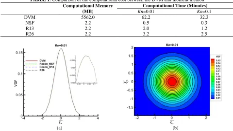
The velocity profiles of force-driven Poiseuille flow are shown in Figure 1. When Kn=0.01, both R13 and R26 have the capacity to the capture non-equilibrium phenomenon accurately, and the velocity at the centre of the channel is slightly underpredicted by NSF equation. In Figure 2, it can be seen that the reconstructed VDFs from different order of Hermite polynomials can accurately reproduce the VDF features. However, when Kn=0.1, the NSF equations can only capture the basic trends of the velocity, R13 and R26 equations are able to produce better solutions, with 3.64% and 1.07% maximum error, respectively, as shown in Figure 1. (b). The The convergence criterion for the steady-state is defined by

(

)

1 6

1

1 10

+

− +

−

+ =







n n

n

E n ,

u u

u (19)

[image:6.612.65.545.79.350.2]

TABLE 1. Comparison of the computational cost between the DVM and moment method

Computational Memory (MB)

Computational Time (Minutes)

Kn=0.01 Kn=0.1

DVM 5562.0 62.2 32.3

NSF 2.2 0.5 0.3

R13 2.2 2.0 1.2

R26 2.2 3.2 2.5

(a) (b)

FIGURE 2. Comparison of VDFs from DVM and moments at Kn=0.01: (a) VDFs along the velocity cross-section. (b). VDFs contour: lines and colors are the VDFs constructed from R26 and VDM, respectively

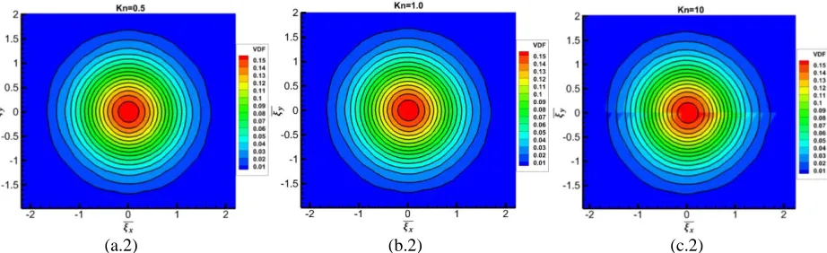
A detailed comparison for expanded VDFs in different order of Hermite polynomials has been given in Figure 3 with different Kn numbers. When Kn1.0, the reconstructed VDFs can give a relatively accurate predict in comparison with DVM. For large Kn, ie. (Kn=10), the VDF calculated from DVM is far away from equilibrium, and both R13 and R26 are fail to produce accuracy VDFs, and thus lead to inaccurate solutions when using R13 and R26 to predict highly rarefied gas flows. To overcome this problem, a great number of moments in combine with boundary conditions are necessary to reconstruct the accuracy VDFs in highly rarefied gas flows.

[image:6.612.86.531.467.634.2]

[image:7.612.78.539.72.213.2]

(a.2) (b.2) (c.2)

FIGURE 3. Comparison of VDFs from DVM and moments at (a) Kn=0.5, (b) Kn=1.0, (c) Kn=10: (1). VDFs along the velocity cross-section. (2). VDFs contour: lines and colors are the VDFs constructed from R26 and DVM, respectively

Flow Past a Circle Cylinder

In addition to the force-driven Poiseuille flow, the comparative study between the DVM and the moment method is also performed on flow past a 2D circle cylinder, which is a standard problem to validate numerical accuracy and efficiency. The cylinder centre sits at x=0,y=0. The diameter of the cylinder, D, is defined as the characteristic flow length. The Knudsen number is chosen to beKn=0.05. With the free stream flow velocity as the reference velocity, the Reynold number and Mach number areRe=20，Ma=0.5642, respectively. The inlet and outlet boundary condition for the DVM were set as Maxwell equilibrium distribution function with density



=1, temperatureT =1. Fully diffusive wall boundary condition is employed, and the temperature of the wall was set equal to the free stream temperature. The discrete velocity space is discretized the range of _−6 2RT_ref,6 2RT_ref_2

with 40 40 non-uniform distributed Newton–Cotes quadrature points. In the spatial space, 1600 1600 uniform grids are applied, and the computational domain is 20 times larger than D. The surface of the cylinder is approximated by staircases. In the moment method, body fitted grid is employed. The computational domain is 1500 times larger than D and the independence of the results on the spatial grids has been tested in Ref [21], however, in the DVM simulation, traditional Cartesian coordinate is used, which may cause extra error in the simulation.

[image:7.612.126.488.454.621.2]

(a) (b)

FIGURE 4. Temperature contour obtained from R26 and DVM: (a) Moment method, (b) DVM

[image:8.612.99.505.131.415.2]

(x= −5,y=0) is chosen on the central line of the cylinder. When Kn=0.05, VDF can be recovered by Hermite polynomials using moments. Meanwhile, the moment method needs about 6 hours to get the steady-state solutions, and the DVM needs about 20 hours to get the steady-state solutions. Thus, in the early transition- and slip-regimes, moment method can be employed to capture the non-equilibrium phenomena to save the computational resource.

FIGURE 5. The velocity and temperature profiles along the central line of the cylinder obtained from DVM and R26

FIGURE 6. (a). VDFs along the velocity cross-section (b). VDFs contours: colors and lines are obtained from VDM and R26

CONCLUSIONS

The main objective of this work is to quantify the computational performance of the moment method and the DVM, so that the accuracy of the moments method has been evaluated both in macroscopic and microscopic levels. Our simulation results show that both R13 and R26 equations can accurately reproduce the results under low Knudsen numbers in force-driven Poiseuille flows. When the Kn=0.1, with 51 grid points along the channel cross section, the NSF model fails to produce the accuracy results, and the R13 and the R26 moment equations can relatively get the accurate results with 3.64% and 1.07% maximum errors, respectively. A detailed comparison for the moment method and the DVM has been carried out in microscopic level with a wide range of Knudsen numbers. When Knudsen is less than 1, the moment method is able to reconstruct a relatively accurate VDF from Hermite polynomials. However, as the Knudsen number increases to highly rarefied flow regimes, the R13 and the R26 moment equations are no longer valid. The simulation of flow past a circle cylinder shows that, when

0.05, Re 20

Kn= = , moment method has the ability to capture the accurate non-equilibrium phenomenon and produce accurate results in comparison with the DVM. In summary, the moment method is preferable for slip regime and early transition regime, as it can recover the VDF with high accuracy and reduce the computational cost.

ACKNOWLEDGMENTS

REFERENCES

1. G. A. Bird, Molecular gas dynamics and the direct simulation of gas flows, (Clarendon, Oxford, 1994). 2. L. Zhu, P. Wang, Z. Guo, Journal of Computational Physics, 333, 227-246 (2017).

3. Z. Guo, K. Xu, R. Wang, Physical Review E, 88, 033305-1 - 03305-11 (2013). 4. L. Wu, Y. Zhang, J. M. Reese, Journal of Computational Physics, 303, 66-79 (2015).

5. L. Wu, C. White, T. J. Scanlon, J. M. Reese, Y. Zhang, Journal of Computational Physics, 250, 27-52 (2013). 6. P. L. Bhatnagar, E. P. Gross, M. Krook, Physical Review, 94, 511 (1954).

7. L. H. Holway Jr, Physics of Fluids, 9, 1658-1673 (1966). 8. E. Shakhov, Fluid Dynamics, 3, 95-96 (1968).

9. P. Wang, M-T Ho, L. Wu, Z. Guo, Y. Zhang,Computers and Fluids, 161, 33-46 (2018).

10. H. Struchtrup. Macroscopic transport equations for rarefied gas flows, (Springer, New York, 2005). 11. T. Ohwada. Physics of Fluids A: Fluid Dynamics, 5, 217-234 (1993).

12. M-T. Ho, L. Zhu, L. Wu, P. Wang, Z. Guo, Z-H. Li, Y. Zhang, Computer Physics Communications, 234, 14-25 (2019).

13. Grad, H. Comm. Pure Appl. Math, 2, 331-407 (1949) 14. Grad, H. Comm. Pure Appl. Math, 5, 257-300 (1949)

15. H. Struchtrup, T. Manuel, Physics of Fluids, 25, 199-206 (2012). 16. H. Struchtrup, T. Manuel, Physics of Fluids, 15, 2668-2680 (2003). 17. X-J. Gu, D. R. Emerson,Journal of Fluid Mechanics, 636, 177-216 (2009).

18. H. Struchtrup. Macroscopic Transport Equations for Rarefied Gas Flows, (Springer, New York, 2005). 19. X-J. Gu, D. R. Emerson, Nanoscale and Microscale Thermophysical Engineering, 11, 85-97(2007). 20. X-J. Gu, D. R. Emerson, Journal of computational physics, 225, 263-283 (2007).