Rochester Institute of Technology
RIT Scholar Works
Theses Thesis/Dissertation Collections
12-4-2015
Efficient Implementations of Pairing-Based
Cryptography on Embedded Systems
Rajeev Verma
[email protected]Follow this and additional works at:http://scholarworks.rit.edu/theses
This Thesis is brought to you for free and open access by the Thesis/Dissertation Collections at RIT Scholar Works. It has been accepted for inclusion in Theses by an authorized administrator of RIT Scholar Works. For more information, please [email protected].
Recommended Citation
Pairing-Based Cryptography on
Embedded Systems
by
Rajeev Verma
A Thesis Submitted in Partial Fulfillment of the Requirements for the Degree
of
Master of Science in Computer Engineering
Supervised by
Dr. Reza Azarderakhsh
Department of Computer Engineering
Kate Gleason College of Engineering
Rochester Institute of Technology, Rochester New York
December 4, 2015
Approved By:
Dr. Reza Azarderakhsh
Department of Computer Engineering, R.I.T
Primary Advisor
Dr. Marcin Lukowiak
Department of Computer Engineering, R.I.T
Secondary Advisor
Dr. Mehran Mozaffari Kermani
Contents
Contents i
List of Figures v
List of Tables vii
Nomenclature vii
1 Introduction 9
2 Preliminaries of Pairings 13
2.1 Bilinear Pairings . . . 13
2.2 Finite Fields . . . 14
2.3 Elliptic curve Arithmetic . . . 14
2.4 The Group Low . . . 15
2.5 The Tate Pairing . . . 17
2.6 Miller Algorithm . . . 17
2.7 Applications . . . 18
2.7.1 Tripartite Diffie-Hellman . . . 18
2.7.2 Co-GDH Signature Scheme on Elliptic Curves . . . 19
2.7.3 BLS Short Signatures on Elliptic curves . . . 19
2.8 Tower Extension Field Arithmetic . . . 20
2.9 Barreto-Naehrig Elliptic Curves . . . 21
2.10 The Ate Pairing . . . 22
2.11 The Optimal Ate-Pairing . . . 23
2.12 Final Exponentiation . . . 24
2.13 Coordinate Systems . . . 25
3 Prime Field Arithmetic 29
3.1 Addition and Subtraction . . . 29
3.2 Finite Field Multipliers . . . 31
3.2.1 Schoolbook Method . . . 31
3.2.2 Comba’s Method . . . 32
3.2.3 Montgomery Method . . . 33
3.2.4 Karatsuba Method . . . 35
3.3 Reduction . . . 35
4 NEON based ARM Architectures 37 4.1 ARMv7 Architecture . . . 38
4.2 ARMv8 Architecture . . . 39
4.3 ARMv7/v8 NEON programming basics . . . 41
4.3.1 NEON intrinsic method . . . 42
4.3.2 NEON Assembly . . . 42
5 Field Level Optimizations1 47 5.1 Challenges in implementing pairing for higher fields . . . 48
5.2 Proposed NEON implementation of Schoolbook multiplier. . . 49
5.3 Karatsuba multiplier using NEON . . . 50
5.4 Reduction using NEON . . . 52
5.5 Fq2 andFq6 field multiplication without reduction . . . 52
5.6 Squaring . . . 54
5.7 Inversion . . . 56
6 Results and comparison 59 6.1 Miller Loop Operations . . . 59
6.2 Implementation Timings . . . 61
6.2.1 Timing comparison for different multipliers . . . 63
6.2.2 Timing comparison for NEON based Karatsuba and Schoolbook mul-tipliers . . . 64
6.2.3 Timing results for pairings . . . 65
6.2.4 Speed records for pairings computations on different security levels . 68
7 Conclusion and Future Work 69
Contents iii
References 71
A Code for 128-bit SOS multiplier 77
List of Figures
1.1 Tripartite Diffie–Hellman protocol over Elliptic curves. . . 10
2.1 Operation flow of Elliptic Curve based cryptosystem. . . 16
4.1 Graphic interpretation of ARMv7 NEON Register Packing. . . 37
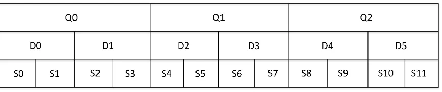
4.2 Graphic interpretation of ARMv8 scalar Register Packing. . . 40
4.3 Graphic interpretation of ARMv8 Register Packing. . . 40
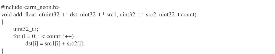
4.4 Addition of unsigned integer (uint32_t) array using C. Assumed that number of words in input are multiple of 4. . . 42
4.5 Addition of unsigned integer (uint32_t) array using Intrinsic NEON. Assumed that count is multiple of 4. . . 43
4.6 Assembly code in .S file for ARMv7. . . 44
4.7 Assembly code in .S file for ARMv8. . . 45
List of Tables
4.1 ARMv7 NEON instruction options. . . 38
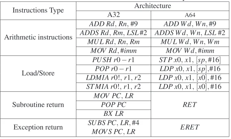
4.2 Basic difference in ARMv7 and ARMv8 assembly instructions. . . 39
4.3 ARMv8 vector shape and Name convention. . . 41
4.4 ARMv8 NEON instruction options. . . 41
6.1 Operation counts for 254-bit, 446-bit, and 638-bit prime fields . . . 60
6.2 Timings for affine and projective pairing on different ARM processors and comparisons with prior literature. Times for the Miller loop (ML) in each row reflect those of the faster pairing. . . 62
6.3 Timing Comparision for Multiplier of diffrerent fields . . . 63
6.4 Timings Comparison for Multiplier of 446-bit and 638-bit field size. . . 64
6.5 Timings comparison for Multiplier for ARMv8 architecture. . . 64
6.6 Timings for Schoolbook Multipliers on Different platforms. . . 64
6.7 Timings for Karatsuba Multiplier for different platform . . . 65
Chapter 1
Introduction
Cryptography is a key technology for achieving information security in computer systems, electronic commerce, and in the emerging information security systems. Elliptic curve cryp-tography [1] are advantageous among public key cryptosystems for its faster key generation, shorter key size for same security level compared to RSA and low on CPU and memory con-sumption. The discrete logarithm Problem (DLP) is intractable for some group of points on elliptic curve defined over a finite field. Intractability of Diffie-Hellman problem (DHP) [2] is the basis of Diffie-Hellman key agreement protocol which allow two parties (Alice and bob) to establish a shared secret key by communicating over a public channel that is being moni-tored by eavesdropper (Eve). This protocol is efficient to share key among two parties in one round but if we have three parties to share the key over a public channel Diffie-Hellman key agreement protocol takes two step. Antoine Joux [3] devised a simple protocol to share the key between three parties in one round using pairings. Three party key exchange protocol using pairing is shown in in Figure1.1. Alice, Bob and Chris have private keys as a,b,c and calculate aP, bP and cP using scalar multiplication over elliptic curve and share these values over public channel.
Finally all three parties calculate shared key in only one round as:
e(bP,cP) = e(P,P)abc(Alice)
e(aP,cP) = e(PP)abc(Bob)
e(aP,bP) = e(P,P)abc(Chris)
Figure 1.1: Tripartite Diffie–Hellman protocol over Elliptic curves.
identity based encryption scheme explained by Boneh and Franklin [4] increased the popular-ity of pairing based cryptography. Many pairing based cryptosystems are being proposed fol-lowing Boneh and Franklin which would be difficult to design using conventional cryptograhic primitives. For instance [5] identity-based key agreement, searchable public-key encryption, short signature scheme, certificate less encryption, blind signature, attribute based encryption [6], are some of the interesting applications of pairing based cryptosystems. Elliptic curve cryptosystems provides relatively small block size over other cryptosystems, high-security public key schemes that can be efficiently implemented. Elliptical curves over finite field [7] are most secured and efficient way to implement bilinear pairings for these applications.
Pairing based cryptosystems are being implemented on different platforms such as low-power and mobile devices. Recently, hardware capabilities of embedded devices have been emerging which can support efficient and faster implementations of pairings. The basic idea of pairings is the construction of a mapping between two cryptographic groups which allows a cryptographic scheme based on reduction of one complex problem in one group to a different and easier problem in another group. The known implementations of these pairings – the Weil [8], ate [9], Tate and Optimal-ate [10] pairing, – involve fairly complex mathematics. All pairing based applications use a pairing-friendly elliptic curve of prime numbers. There are different coordinate systems [11] can be used to represent points on elliptic curves such as, Jacobian, Affine and Homogeneous. Inversion to multiplication ratio threshold can be used to decide the efficiency of coordinate system [12]. In this work timing results of pairing is being reported for both affine and projective coordinates using BN-curve [13] which is widely used curve for pairing-based algorithms. All fast algorithms to compute pairings on elliptic curves are based on Miller’s algorithm [8] , [14].
11
[17] and [18] [12] [19] for PC and ARM processor based devices respectively. Computation of pairings over binary extension fields, i.e.,F2mis not attractive anymore due to the recent
at-tack presented in [20]. So in this work, we are focused on implementation of pairing on prime fields for low-resource devices using ARM processors. ARM processors are widely used core support for smart phones and tablets class CPU’s. ARM has introduced NEON engine in ARMv6 onward. NEON is general purpose Single Instruction Multiple Data (SIMD) engine which can accelerate signal processing for pairing based protocols [21]. A. H. Sánchez and F. Rodríguez-Henríquez [19] for the first time used NEON to improve the timing results for pair-ing on ARM based devices but this work is only for 254-bit (128-bit security level). To date, there is no work available on higher security levels such as 446-bit and 638-bit which is using NEON engine to improve the pairing timings on low resource devices. General implementa-tion of pairing-based algorithms uses tower like structure for computaimplementa-tions in higher fields so lower level arithmetic computations such as addition, multiplication, squaring, inversion etc. are crucial to improve the timings for higher level algorithms. Among them multiplication plays an important role to determine the efficiency of pairings.
We have different multipliers present in literature, which can be used for lower level mul-tiplication for pairing based algorithm other than multiplier in GMP library. One can refer to [22] for revisited montgomery multiplier which is NEON based implementation of Mont-gomery Multiplier [23]. BN446 and BN638 curve computations require 446-bit and 638-bit multiplication which is not efficient using revisited Montgomery as the algorithm uses the operands with field size as 256-bit, 512-bit. Another implementation is [24] which uses NEON for implementation of modified version of Karatsuba multiplier [25]. A. H. Sánchez and F. Rodríguez-Henríquez [19] uses NEON based implementation of Montgomery multiplier in higher field. In this work we present the implementation of Schoolbook [26] and Karatsuba multiplier [25] using NEON and ASM instructions for different fields and compare their per-formance with above multipliers.
This work1 optimize the pairings algorithm implementations using NEON engine for hand-held devices based on ARM architectures. In this work, we optimize the implementation of pairings presented in [12] for different BN curves such as, BN254, BN446 and BN638. We present a comparison between different multipliers present in the literature and present the tim-ing comparision of pairtim-ings computations ustim-ing each multiplier. Timtim-ings are betim-ing measured for both affine and projective coordinates for O-Ate pairings for different security levels. Our work present 6% improvement over the previous NEON based best timing for BN254 curve [19]. We also present the timing improvement of pairing computations for BN446 and BN638
Chapter 2
Preliminaries of Pairings
In this chapter, we discuss about basics of pairings, their applications and implementations using elliptic curves.
2.1
Bilinear Pairings
LetG1andG2be cyclic groups of prime ordernwritten additively with identity∞, and letG3
be a cyclic group of order n written multiplicatively with identity 1.
Definition 1. A bilinear pairingsecan be defined as:
e:G1×G2→G3
that satisfies the following additional properties: (1) Bilinearity: For allP,P′∈G1andQ,Q′∈G2,
e(P+P′,Q) = e(P,Q)e(P′,Q),
e(P,Q+Q′) = e(P,Q)e(P,Q′).
(2) Non-degeneracy: e(P,P)6=1
Additionally, one wants e to be efficiently computable. From the two properties above, we can have several other useful properties of e.
1. e(P,∞) =e(∞,Q) =1.
3. e(aP,bQ) =e(P,Q)ab f or all a,b∈Z.
4. e(P,Q) =e(Q,P) (only i f G1=G2).
5. Ife(P,Q) =1 for allQ∈G2thenP=∞.
For detail explaination one can refer [27].
2.2
Finite Fields
A field [27] is a set that contains specific elements and equipped with two binary operations,
+(addition) and . (multiplication), which has distinct additive and multiplicative identities, admit additive and multiplicative inverse, and satisfy associative, commutative and distributive laws. For exampleQ(rational numbers),R(real numbers),C(complex numbers) etc.
A f inite f ield [7] is a field with a finite number of elements which has size equal to pm, for some prime p. There is exactly one finite field of size q= pm for each pair(p,m)and we denote this field asFpm orFqwhich is called asGalois f ield and also denoted asGF(q).
Whenq=pm is a prime power, the fieldFpm can be obtain by taking the setFp[X]of all the
polynomials inX with coefficients inFqmodulo any single irreducible polynomial of degree
m.
Elliptic curves over finite fields are of special interest in implementation of cryptographic algorithms. There is no other known faster algorithm than O(√n) for computing discrete logarithms on the elliptic curve which is represented by group of points. In other words elliptic curves provide theoretical maximum possible level of security in public key cryptographic applications.
2.3
Elliptic curve Arithmetic
Elliptic curves group is a good choice for implementation of pairing-based cryptographic al-gorithms because of the simplicity of implementation as explained in [27]. An elliptic curve is the set of points satisfying an equation in two variables with degree two in one of the variables and three in the other.
Definition 2. LetF is a field with characteristics not equal to 2 or 3. An elliptical curve E
overFis defined as set of solutions of the Weierstrass equation:
2.4 The Group Low 15
wherea,b∈F.
The discriminant ofE is defined as:
△=4a3+27b2
An elliptic curve is defined as “smooth” if there is no point at which the curve has two or more distinct tangent lines and△6=0 is the condition to ensure that. In this thesis we will assume
that the chosen curve is “smooth”.
In Equation2.1, if we setZ=0 the result will beX3=0 which has solution as[0 : 1 : 0]. For elliptic curve this point is called as the point at infinity and denoted as∞.
We consider simplified Weierstrass equation withZ6=0 which is defined as:
y2=x3+ax+b (2.2)
So, the elliptic curve can be defined as set of solutions to the equation 2.2 and also the point at infinity. We can also define elliptic curve as set of allK-rational points on E whereK
is an extension ofFas:
E(K):
(x,y)∈K×K:y2=x3+ax+b ∪ {∞}
Elliptic Curve Discrete Logarithm Problem (ECDLP) is defined as: given pointsPandQ
in the group, find a number k such thatPk=Qwhich is called scalar multiplication for elliptic curve. With knownPandQ, one must guess at least the square root of the number of points on average to fine the value ofk. If Pand Q are two point on the elliptic curve, the elliptic curve point addition (ECADD) is defined as R=P+Q and elliptic curve point doubling is defined asQ=2P.
2.4
The Group Low
LetE be an elliptic curve defined over the fieldK. Chord-and-tangent rule is being used to add two points inE(K)to give a third point in the sameE(K). This addition operation with set of pointsE(K)and∞forms an abelian group to construct elliptic curve cryptographic systems. LetPandQbe two distinct points on curveE, then the group low is described as:
1. Identity. P+∞=∞+P=Pfor allP∈E(K).
Cryptographic Transformations Digital Signature generation Key Exchange and verification
Scalar multiplication of elliptic curve point Encryption / Decryption
Point doubling
Addition Arithmetic in elliptic curve
point group
Arithmetic in finite field
Mov,mul,shr,shl,add,sub... CPU Commands
Multiplication Squaring Inversion Point addition
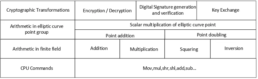
[image:24.595.91.511.121.250.2]Operation flow of elliptic curve cryptosystem
Figure 2.1: Operation flow of Elliptic Curve based cryptosystem.
3. Point addition. LetP= (x1,y1)∈E(K)andQ= (x2,y2)∈E(K), whereP6=±Q. Then
P+Q= (x3,y3)where
x3=
y2−y1 x2−x1
2
−x1−x2 and y3=
y2−y1 x2−x1
(x1−x3)−y1.
4. Point doubling.LetP= (x1,y1)∈E(K), whereP6=−P. Then 2P= (x3,y3),where
x3=
3 x21+a
2y1
2
−2x1 and y3=
3 x21+a
2y1
(x1−x3)−y1.
2.5 The Tate Pairing 17
2.5
The Tate Pairing
The Tate pairing is an example of bilinear pairings defined on the group of points over an elliptic curve for a finite field. Let E is and elliptical curve over the finite field Fq and the
order ofE ishnwherenis a prime such that its not equal to the characteristics ofFqandhand
nare co-prime. We defineµnasµn=u∈F¯q: un=1 which is a group ofnth−root of unity.
Definition 3. Definition of the fieldF =Fq(µn)as the extension of the field Fqgenerated by
thenthroots of unity. Ifkis the degree of this extension thenkis called the embedding degree ofEwith respect ton. In other words embedded degree is the smallest value of integerksuch thatn|qk−1.
We can define Tate pairinge(P,Q)as
e(P,Q) = fP(DQ)
qk−1
n =
fP(Q+R)
fP(R)
qkn−1
It can be observed that the value of Tate pairing does not depend on either function fP or
DQ, so it is well defined and it is bilinear and non-degenerate [28]. It is shown in [28] that for
k>1,DQcan be replaced withQwhich redefines Tate pairing ase(P,Q) = fP(Q)
qk−1
n where
fPis called Miller function and we can use Miller algorithm to calculate this function.
2.6
Miller Algorithm
Miller’s algorithm [8] is the most efficient algorithm to evaluate at a certain point a function assiciated with prinipal divisor. In a general method, any function fn,Pwith the divisorn(P)− (iP)−(i−1)(∞)is called the Miller function. Miller function is the key component of Tate pairing computation. The key idea of Miller’s algorithm is to construct the function fn,Pusing
doubling and addition.
Miller algorithm construct fnusing double-and-add approach and f1=1. The function fn
has divisor asn(P)−([n]P)−(n−1)∞=n(P)−n(∞). As explained in Algorithm2.1, Miller algorithm uses loop (step 2 to step 9) which is called Miller Loop. In order to compute Tate pairing, Miller algorithm computes the value of fn(Q)instead of computing all the values for
each step as fiwhich makes it easy to compute. The step-10 of the algorithm is called final
Algorithm 2.1Miller’s Algorithm for the O-Ate pairing [8].
Inputs:PointsQ,P∈E[n]and integer
n= (nl−1,nl−2,···,n1,n0)2∈Nandnl−1=1
Output: fn,Q(P).
1:T ←Q, f ←1
2:fori=l−2downto0do
3: f ← f2·lT,T(P)
4: T ←2T
5: ifli6=0
6: f ← f ·lT,P(P)
7: T ←T+Q
8: end if
9:end for
10: f ← fqkn−1
11:return f
2.7
Applications
The bilinear pairings such as Tate pairing or Weil pairings on elliptical curves have been very efficient in cryptographic applications. Bilinear pairings has been used for implementing Sev-eral ID-based cryptosystems. Certificate-based public key infrastructure (PKI) can be replaced by the ID-based public key cryptosystem especially when moderate security and efficient key-management are required. These are some basic application based on bilinear pairing:
2.7.1
Tripartite Diffie-Hellman
Joux [3], use the pairings in the development of the three-party, one-round key-exchange pro-tocol. This protocol is a three-party version of Diffie-Hellman and its security is based on the following assumption:
Definition 4. Letebe a bilinear pairingse:G1×G1→G2withP∈G1. GivenP,aP, bP,cP, it is computationally infeasible to computee(P,P)abc.
These are steps for protocol:
1. The three parties agree on a common pointP∈G1.
2. Each party chooses a secret integera,b,cand broadcastsaP,bP,cP.
2.7 Applications 19
e(P,P)abc=e(aP,bP)c=e(aP,cP)b=e(bP,cP)a.
2.7.2
Co-GDH Signature Scheme on Elliptic Curves
LetsG1, G2 are subgroups of the elliptic curveE/Fq, and assume there is a mapping which
can be used to place the messageMas a point on the elliptic curveE. In other words, we can sayMis being represented as a point on elliptic curveG1. Further discussion can be found in
[29].
Private Key:Alice randomly selects an integerx←R Zq.xis secret key asx∈Zq
Public Key:Compute public key isV =xQwhere Q generatesG2.
Signature: LetM∈G1 be the message and computeσ ←xM∈E(Zq) whereh∈G1. The
x-coordinate ofσ is the signatureSonM soS∈Fq
Verification:Given a public keyV∈G2, a messageM∈G1and signatures∈Fq, finda,y∈Fq
such thatσ = (s,y)is a point which has order pinE(Fq).
If the signature is valid then we would have
e(σ,Q) =e(M,V)ore(σ,Q)−1=e(M,V)
as required for verification. This signature is efficient as it requires only one point on elliptic curve which is half of the size of DSA signature.
2.7.3
BLS Short Signatures on Elliptic curves
Signature schemes are another use of pairings. Most discrete logarithm signature schemes are variants of the ElGamal scheme. Boneh, Lynn and Shacham presented a signature scheme which uses one group element as the signature and groups elements are represented as the same number of bits as an integer modulon which is called as BLS short signature scheme [30].
Letebe a bilinear pairings ase : G1×G1→G2 whereG1=<P>be the prime ordern
subgroup generated by pointP∈E(Fq)then alsoG1∈E(Fqk)wherekis the embedding degree
ofQandG2is a prime order subgroupG2∈E(Fqk)with linear independent points of the ones
in groupG1. Let’sH be a cryptographic hash function H:{0,1}∗→G1. The general BLS algorithm works as follows:
Private Key:Alice randomly selects an integerx←R Zq.xis secret key asx∈Zq
Signature: Let m∈{0,1}∗ be the message and compute h←H(m) whereh∈G1. Then
S=xhis the signature.
Verification:Computeh=H(m).Then verify thate(P,S) =e(A,h).
If the signature is valid then we would have
e(P,S) =e(P,aH(m)) =e(aP,H(m)) =e(A,h)
as required for verification.
2.8
Tower Extension Field Arithmetic
Cryptosystems based on elliptic curve can be so generic that can work for different point size on curves such as, 128-bit, 164-bit and 192-bit. When using pairings based protocols, its necessary to perform arithmetic in higher fields such as, Fqk for moderate value of k. It is
important to represent the field in such a way that arithmetic can be performed in efficient way. One of the most efficient way is to use a tower of extension field [31] which explains that higher level computations can be calculated as a function of lower level computations so that efficient implementation of lower level algorithms can impact the performance of algorithms in higher fields.
Miller Algorithm is being executed using arithmetic inFq12 field during the accumulation
step of the algorithm. Extension field arithmetic are very important to improve the perfor-mance of pairing. Fqk should be represented with the tower of extensions with the use of
irreducible binomials as explained in [32] and can be expressed as:
Fq2 = Fq[i]/(i2−β),whereβ =−1
Fq4 = Fq2[s]/(s2−ξ),whereξ =i+1 Fq6 = Fq2[u]/(u3−ξ),whereξ =i+2 Fq12 = Fq4[t]/(t2−s)orFq6[w]/(w2−u)
The conversion from one towering Fq2 →Fq6 → Fq12 to another Fq2 → Fq4 → Fq12 is
2.9 Barreto-Naehrig Elliptic Curves 21
2.9
Barreto-Naehrig Elliptic Curves
Pairings based cryptography requires pairing-friendly curves [33] and these curves are param-eterised by the factor embedding degree k. Pairing definitions show that randomly chosen elliptic curve might be suitable for implementing pairing-based protocols. But if the embed-ding degree of the curveEis very large, it is not possible to implement field arithmetic in the size ofFqk.For the implementation of elliptic curve the embedding degree, with respect ton,
should be small enough so that curve arithmetic in extension field should be easy to implement yet large enough that Discrete Logarithmic Problem is intractable inFqk. Since the larger
sub-groups provide high level of security so the elliptic curveE should have a large prime order subgroup for arithmetic implementation of the curve. Elliptic curves with suitably low em-bedding degree are very rare. Balasubramaniam and Koblitz [34] showed that one can expect
k≈qfor a randomly selected prime-order elliptic curve over a randomly selected prime-order field and also the probability thatk≤log2qis vanishing small.
There are many methods to generate elliptic curve in literature. David Freeman [33] showed the comprehensive review of the different curves. Barreto and Narhrig [13] devised a method to generate elliptic curve which supports pairings over prime field with prime order
k=12 which is called as Barreto-Narhrig or BN-curve. We have used BN-curves for our im-plementations as BN-curve is suitable to achieve high security and efficiency of cryptographic algorithms. BN-curves enable all kind of pairing-based cryptographic schemes and protocols (including short signatures) [35]. In this work we are focusing on implementation of pairings on BN-curve which has prime order and every point in the curve has ordern. The equation of BN-curve isE : y2=x3+b, withb6=0. The trace of the curve, the characteristic ofFqand
the curve order are parameterised as:
t(x) = 6x2+1
n(x) = 36x4+36x3+18x2+6x+1
q(x) = 36x4+36x3+24x2+6x+1
Pairings on BN-curves are computed over points inE(Fq12)because BN-curves have
em-bedding degree as 12 so the pairings on a BN curve over a 256-bit prime fieldFq takes its
values in the field Fq12 with size 256×12=3072. To construct a pairing-friendly elliptic
b+1 is a quadratic residue. Furthermore, P= (1,√b+1) is a point on curveE that can be used as generator forE(Fq). As mentioned in [36], BN-curves are ideal for implementation
of optimized variant of Tate pairing which is referenced as O-Ate pairing.
2.10
The Ate Pairing
Pairings can be computed in polynomial time using Miller’s algorithm as explained in2.6. Many other techniques have been suggested for optimizing the computation of pairings. Among those, one of the most elegant technique is to shorten the iteration loop in Miller’s algorithm to compute pairings efficiently. The Ate Pairing is referred as optimized version of Tate Pairing in which Miller loop is designed to be shorter than that of used in the Tate pairing. We derive the Ate Pairing using [10] and further explained Optimal-Ate pairing.
To minimize the number of addition steps in Miller’s algorithm, we choosento have a low Hamming weight. In Miller loop, the computation ofnP=∞is being done using double-and-add method which can be simplified choosingP such that it’s coordinates lie in a sub-field ofFqk. As mentioned in above section, we can choose P= (1,
√
b+1) as the generator of the subgroup. In Ate pairing, the parameters are restricted to Frobenius eignespace. We will choose the first parameterQ∈G2and second parameterP∈G1.
Lemma 5. [27] fab,Q= fab,Q· fb,aQ f or all a,b∈Z.
This leads to following lemma [10].
Lemma 6. e(Q,P)m= f
mn,Q(P)
qk−1
n where e(Q,P)is the Tate Pairing with Q∈G2, P∈G1
and m∈Z.
which defines the pairings on the curve. The following fact defines the pairings in simpler
way:
Fact 7. [10] fa,Πq(Q)(P) = fa,Q(P)qfor all a∈Zand Q∈G2.
Using above fact we can gete(Q,P)m= f
λ,Q(P)
qk−1
n kq k−1
.
Sincenandqare prime, we have thatn∤qandn∤k. Thus we can define:
a(Q,P) =e(Q,P)m((k−1q−(k−1))modn)= fλ,Q(P)qkn−1.
2.11 The Optimal Ate-Pairing 23
q(x)∼=6x2(modn(x))so we takeλ=6x2. This reduces the Miller loop length from log(36x4+
36x2+18x2+6x+1)to log(6x2).
There is further possibility to optimize the Miller loop as sown in [10] which is called Optimal Ate or O-Ate pairing.
2.11
The Optimal Ate-Pairing
The Optimal Ate or O-Ate pairing is an improved version of Ate pairing. Let’s consider the
mth power of Tate Pairing andσ=mnand supposeσ =∑l
i=0
ciqi is the base-q expansion ofσ.
Ifsi= l
∑
j=i
cjqj, we have:
e(Q,P)m = ( l
∏
i=0fci
qi,Q(P) qk−1
n )(
l
∏
i=0fcqi
i,Q(P)
l−1
∏
i=0l[ciqi]Q,s
i+1Q(P)
vsi,Q(P)
)qkn−1
The left side of above expression is bilinear pairing. The right side of expression is a product of powes of Ate pairing so it is also bilinear. The factors of second set should also be a bilinear pairing. As explained in [10] letσ =mnwithn∤mthen:
aO: G2×G1→µngiven by:
(Q,P)7→( l
∏
i=0fcqi
i,Q(P)
l−1
∏
i=0l[ciqi]Q,s
i+1Q(P)
vsi,Q(P)
)qkn−1
defines a bilinear pairings called the O-Ate pairing. Furthermore if mkq−1✚≡✚ q
k−1
r l
∑
i=0
iciqi−1modnthen the pairing is non-degenerate.
The O-Ate Pairings on BN-Curves
From BN-curve definition:Q(x) = 36x4+36x3+24x2+6x+1
N(x) = 36x4+36x3+18x2+6x+1
Q(x) = 6x2modN(x),
Q(x)2 = 36x3−18x2−6x−1 modN(x), Q(x)3 = 36x3−24x2−12x−3 modN(x).
Therefore,
6x+2+Q(x)−Q(x)2+Q(x)3=0 modN(x). (2.3)
Lets σ =6x+2+Q(x)−Q(x)2+Q(x)3 which gives the following expression for O-Ate pairing on BN-curves:
(Q,P)7→ f6x+2,Q(P)f1q,Q(P)fq
2
−1,Q(P)f q3
1,Q(P)g(P).
We know f1,Q= f−1,Q=1, so we can ignore these in above expression. The expression
forg(P)is given by:
g(P) =l[6x+2]Q,[q−q2+q3]Q(P)l[q]Q,[−q2+q3]Q(P)l[−q2]Q,[q3]Q(P).
The expression ofg(P)can be simplified further using following lemma:
Lemma 8. g(P)qkn−1 =h(P) qk−1
n where h(P) =l[6
x+2]Q,qQ(P)l[6x+2]Q+qQ,−q2Q(P).
By the above lemma,g(P)can be replaced byh(P)when computing the O-Ate pairing on BN-curves. Finally(Q,P)can be represented as:
(Q,P)7→ f6x+2,Q(P)·h(P). (2.4)
The above expression is the expression for O-Ate pairing on BN-curves. In this work we have used the pairings equation as2.4for efficient implementation.
2.12
Final Exponentiation
Exponentiation is the final step in Miller algorithm [8] in which it is required f to be raised to the exponent qkn−1. BN-curves have embedding degree ask=12. We can write k=2d and implementFqk as a quadratic extension ofFqd whered=6. Then, exponent can be represent
2.13 Coordinate Systems 25
qk−1
n =
q2d−1
n =
(qd−1)(qd+1)
n .
k was chosen to be minimal such that n|qk−1, we see that n∤qd−1 and n is a prime,
n|qd+1. So, we split the exponentiation in two parts as exponentiation by qd−1 and then
qd+1
n .
If a∈Fqk can be represented as a=α+βswhere α,β∈Fqd and s is an adjoined square
root. The Frobenius endomorphism can be represented as
(α+βs)qd =α−βs (2.5) Equation2.5 gives us ability to compute fqd−1 in an easy way. The next step would be computing(f.h)qdn+1 and represent as
qd+1
n = (q
2+1)q4−q2+1
n
Computing fq
4−q2+1
n relies on computing O-Ate pairing to some suitable power will still
give a bi-linear pairing. To make the computation easy, we will consider multiple of q4−qn2+1 to compute the value. Grewal et al. [12] present the implementation can be performed as
f → fx→ f2x→ f4x→f6x→f6x2 → f12x2→f12x3 (2.6)
Then final exponentiation can be represented as
a f6x2f bpap2(b f−1)p3. (2.7)
which costs 6 multiplication and 6 Frobenius operations.
2.13
Coordinate Systems
doubling for all the three coordinates.
Projective coordinates provides easy way to represent the points on elliptic curves as it represents the ratios of the numbers instead of numbers. The projective coordinate system allow the carry denominator to the third coordinate as:
x z,
y z,1
7−→(x,y,z)
For example 5 can be represented as either 5=5/1 or as 4=8/2, which could be repre-sented as(5,5,1). The infinity point is being represented as third coordinate as 0 as dividing anything with zero indicate infinity. Affine coordinates can be transform to projective coordi-nates and represented as:
[X:Y :Z]7−→[X/Z:Y/Z: 1]7−→ {X/Z:Y/Z}
and{x,y} 7→[X :Y : 1].
The best coordinate system for efficient implementation of pairings depends on computa-tional environment e.g., CPU architecture. As mentioned in [36] if the crossover inversion to multiplication (I/M) ratio is greater than 10.8, projective coordinates are gives better compu-tation timing results for pairing. In this work the results of projective coordinates are better than affine coordinates. In general, actual and crossover I/M ratios gets smaller as field size increases because of the inversion formula for higher extensions. As a result, as the degree of the extension field used for the bulk of the arithmetic in a pairings computation increases, the case for using affine coordinates gets stronger.
2.14
Curve Arithmetic
For the remainder of this thesis, letm,s,a,iandrdenote the times for multiplication, squaring, addition, inversion and modular reduction inFq, respectively. Let ˜m,s˜,a˜,i˜and ˜rdenote times
for multiplication, squaring, addition, inversion and modular reduction inFq2 , respectively.
2.14 Curve Arithmetic 27
The authors of the original implementation [[12], [36] ] examined the implementation of Jacobian, Affine and Homogeneous coordinates systems and it is shown that homogeneous coordinates are most efficient for the given implementation. Explicit formulas and main com-putation costs are being presented by the author for different coordinate systems. For details operation counts and implementations, one can refer [[36], [37]].
Chapter 3
Prime Field Arithmetic
In this chapter, we discuss the arithmetic over prime fields. For pairing computations all of the higher level arithmetic operations are done over prime fields.
3.1
Addition and Subtraction
Addition and substation are most basic algorithms for any prime field algorithm. An assign-ment of the form “(ε,z)←w” for an integerwis understood as:
z←wmod 2W, and
ε ←0i f w∈[0,2W),otherwiseε ←1.
whereW is the word size of machine. If w is defined asw=x+y+ε′forx,y∈[0,2W) and
ε′∈{0,1}, then w=ε2W +z andε is called the carry bit for single word addition. Modular
Addition for multi-word numbers is defined as((x+y)modq) and subtraction is defined as
((x−y)modq).
Algorihm3.1 explains addition in prime field. As shown in step-1, we add first word of the inputs and save the carry. For loop in Step-2 go over all the words, perform the addition on current words and also adds the carry of previous addition. Finally if the carry flag is one or the addition result is greater than prime (q), step-5 perform the reduction step.
Algorithm 3.1Addition inFqfield[1].
Inputs:Modulusq, and integersA= (an−1, ...,a1,a0)and
B= (bn−1, ...,b1,b0). A,B∈[0,q−1]
Output:C= (A+B)mod q. 1:(ε,c0)←a0+b0
2:fori=1upton−1do
3: (ε,ci)←ai+bi+ε
4:ifε=1orC≥q
5: C←C−q
6:Return(C)
Algorithm 3.2Subtraction inFqfield.[1].
Inputs:Modulusq, and integersA= (an−1, ...,a1,a0)and
B= (bn−1, ...,b1,b0). A,B∈[0,q−1]
Output:C= (A+B)modq. 1:(ε,c0)←a0−b0
2:fori=1upton−1do
3: (ε,ci)←ai−bi−ε
4:ifε=1 5: C←C+q
3.2 Finite Field Multipliers 31
Algorithm 3.3Schoolbook Multiplication Method3.3.
Inputs:Two n-digit argumentsA= (an−1, ...,a1,a0)and
B= (bn−1, ...,b1,b0).
Output:P=A.B= (p2n−1, ...,p1,p0).
1:P←0
2:fori=0upton−1do
3: s←0
4: for j=0upton−1do
5: (s,c)←aj×bi+pi+j+s
6: pi+j←c
7: end for
8: pn+i←s
9:end for
3.2
Finite Field Multipliers
Pairings based cryptosystems are computation-intensive algorithms especially when execu-tion is taking place on embedded processors with low resources. The basic reason of com-putation rich algorithms are the operand size of underlying comcom-putations, e.g., finite field multiplication, exponentiation. Among these, multiplication is important building block of elliptical curve cryptosystems and needs careful optimization in pairing-based cryptographic algorithms. Finite field multiplication in pairings algorithms are defined as c=a.b mod q
and faster implementation results in improving the performance of pairings algorithms espe-cially on embedded platforms. In this section we will analyze four multipliers as Schoolbook method [26], Comba [38], Montgomery [23], Karatsuba [25].
3.2.1
Schoolbook Method
The schoolbook method for finite field multiplication is also known as operand scanning method. Schoolbook multiplier can be represented as in Equation 3.1 where we have input arguments asA=AH·2n/2+AL andB=BH·2n/2+BL and the outputC=A.B.
C=AH.BH.2n+ (AH.BL+AL.BH)2
n
2+AL.BL (3.1)
As explained in Algorithm3.3, it consist of two for loops and each of them iterate over the digits of input arguments of n−bit. In each iteration of outer for loop at step-2, the digit
bi of second operand is multiplied with all the digits of first argument and n-bit results is
Algorithm 3.4Comba Multiplication Method [38].
Inputs:Two n-digit argumentsA= (an−1, ...,a1,a0)and
B= (bn−1, ...,b1,b0).
Output:P=A.B= (p2n−1, ...,p1,p0).
1:(s,c,t)←0
2:fori=0upton−1do
3: for j=0uptoido
4: (s,c,t)←(s,c,t) +aj×bi−j
5: end for
6: pi←t
7: t←c,c←s,s←0 8:end for
9:fori=nupto2n−2do
10: for j=i−n+1upton−1do
11: (s,c,t)←(s,c,t) +aj×bi−j
12: end for
13: pi←t
14: t←c,c←s,s←0 15:end for
16: p2n−1←t
non-reduced result of multiplication.
3.2.2
Comba’s Method
Comba [38] first describe one alternative method for finite field multiplication which is called Comba’s method. Comba’s method is also known as product scanning method. Algorithm3.4
illustrates comba algorithm to multiply twon-bit numbers and typically faster than schoolbook method. In step-2, the outerforloop is iterating through each element of output pi and inner
loop implements the algorithm as much simpler as schoolbook multiplier. Thei−thdigit of outputpiofP=A.Bis the accumulation of all inner loop productsaj×bi−jwhere 0≤ j≤ias
shown in step-4 and step-11. The carry is added eventually to the digit from the calculation of previous digit inside the loop. Algorithm3.4uses threew−bitregisters(s,c,t)for the storage of sum of 2w−bit and operations at step-7 and step-14 are the right shift of the registers
(s,c,t).
3.2 Finite Field Multipliers 33
Algorithm 3.5SOS Montgomery Multiplier [39].
Inputs:Two n-digit argumentsA= (an−1, ...,a1,a0)and
B= (bn−1, ...,b1,b0).
Output:P=A.B= (p2n−1, ...,p1,p0).
1:fori=0upton−1do
2: C←0
3: for j=0upton−1do
4: (C,S)←Pi+j+aj×bi+C
5: Pi+j←S
6: end for
7: Pi+n←C
8:end for
9:Return P
3.2.3
Montgomery Method
Montgomery multiplication algorithm is typically faster than both schoolbook and comba mul-tiplication methods. As described in [23], there are five different versions of Montgomery multiplier as:
• Separated Operand Scanning (SOS)
• Coarsely Integrated Operand Scanning (CIOS)
• Finely Integrated Operand Scanning (FIOS)
• Finely Integrated Product Scanning (FIPS)
• Coarsely Integrated Hybrid Scanning (CIHS)
Separated Operand Scanning (SOS) is most usable for pairings when we use lazy reduction technique. Coarsely Integrated Operand Scanning (CIOS) method is improvement over SOS which gives modular multiplication result of input arguments. We use SOS multiplier for NEON implementation. SOS multiplier algorithm is defined in Algorithm3.5 which shows twoforloops, in step-1 and step-3, iterate through the input arguments and combine the mul-tiply of each word with previous carry in step-4. Carry is being handled each time after inner loop is being finished as shown in step-7.
Algorithm 3.6CIOS Montgomery Multiplier [39].
Inputs:Two n-digit argumentsA= (as−1, ...,a1,a0)and
B= (bs−1, ...,b1,b0).
Output:P=A.B= (p2s−1, ...,p1,p0).
1:fori=0uptos−1do
2: C←0
3: for j=0uptos−1do
4: (C,S)←Pj+aj×bi+C
5: Pi+j←S
6: end for
7: (C,S)←Ps+C
8: Ps←S
9: Ps+1←C
10: C←0
11: m←P0×n′0modW
12: for j=0uptos−1do
13: (C,S)←Pj+m×nj+C
14: Pj←S
15: (C,S)←Ps+C
16: Ps←S
17: Ps+1←Ps+1+C
18: for j=0uptosdo
19: Pj←Pj+1
20: end for
21: end for
21:end for
22:Return P
reduction steps in same algorithm which is improvement on SOS method which use reduction method after the multiplication. Instead of computing the entire producta·b, then reducing, CIOS multiplication perform the product and reduction word by word. As shown in Algo-rithm3.6, step-1 and step-3 shows two loops over the input arguments and perform word vise multiplication and addition of carry at step-4. Once the inner loop performs the multiplication another for loop at step-12 performs the reduction step usingm calculated at step-11 as the value of m in thei−thiteration depends only on the value of Pi. Once the three loop ends it
returns the reduced output at step-22.
3.3 Reduction 35
Algorithm 3.7Montgomery ProductMonPro(a¯,b¯)[23].
Inputs:primen,n′,r=2kand ¯a,b¯∈Fq
Output:c¯=MonPro(a¯·b¯). 1:t←a¯·b¯
2: u←(t+ (t·n′modr)·n)/r
3:ifu>nthen
4: returnu−n
5: else
6: returnu
7: end if
3.2.4
Karatsuba Method
Karatsuba Multiplication algorithm reduces the size ofm−bit multiplication to three mul-tiplication of m2–bit but it increases the cost of additions. These half size multiplication can be done using schoolbook or comba multiplier. For Karatsuba multiplier each input is of size m-bit and w is the word size of machine. Each operand for multiplier is writ-ten as A= (A[n−1], ...,A[2],A[1],A[0])and B= (B[n−1], ...,B[2],B[1],B[0])and output is
C= (C[2n−1], ...,C[2],C[1],C[0]), wheren= [m/w]. We can represent the input arguments asA=AH·2n/2+AL andB=BH·2n/2+BL and the outputC=A.Bcan be represented as
Equation 3.2. Karatsuba multiplier can be represent in recursive way and its complexity is
θ(nlog23). There are two typical ways to describe the karatsuba multiplication algorithm as
additive Karatsuba and substrative Karatsuba. Additive Karatsuba multiplier is defined as:
C=A.B=AH.BH.2n+ [(AH+AL)(BH+BL)−AH·BH−AL·BL]·2
n
2 +AL.BL (3.2)
and the subtractive Karatsuba multiplier is defined is
C=A.B=AH.BH.2n+ [AH.BH+AL.BL− |AH−AL|.|BH-BL|]·2
n
2+AL.BL (3.3)
3.3
Reduction
expensive computation. There are faster methods available reduction which includes Barrett Reduction [40], Montgomery reduction [41] and Special Moduli such as Mersenne primes. For pairings there are no special moduli primes and hence we use Montgomery reduction as it is a lot efficient than Barrett when implemented in assembly.
Montgomery reduction technique has replaced the classic heavy reduction technique with less-expensive operations. Montgomery reduction algorithm perform the transformation of the data and calculates Montgomery product. Let the modulusnbe a m-bit integer, i.e., 2k−1≤
n<2kand letr=2ksuch that gcd(r,n) =gcd(2k,n) =1 and this requirement is satisfied when
nis odd. Montgomery multiplier uses the n-residue of an integera<n as ¯a=a·r(modn). The Montgomery reduction introduce a much faster multiplication routine which computes the multiplication of the two integers whose n-residues are known. Lets suppose ¯aand ¯bare two n-residues, then Montgomery product is defined as the n-residue
¯
c=a¯·b¯·r−1(modn) (3.4)
wherer−1 is the inverse ofrmodulonwith the propertyr−1·r=1 (mod n). The resultc
in3.4is the n-residue of the product ofaandbsuch thatc=a·b(mod n), since
¯
c = a¯·b¯·r−1(modn) = a·r·b·r·r−1(modn) = c·r(modn)
Montgomery reduction uses another quantity,n′, which has the property as
r·r−1−n·n′=1
The integersr−1andn′can both be computed by Extended Euclidean algorithm [42]. The computation ofMonPro(a¯,b¯)is explained in algorithm3.7.
Montgomery reduction step is calculatingu as shown in step-2 of Algorithm 3.7. Step3 to step-7 compareu with n and return the reduced result accordingly. This method is very efficient when there are many multiplications are performed for given input, such as modular exponentiation.
Chapter 4
NEON based ARM Architectures
[image:45.595.84.517.581.672.2]ARM introduced single instruction multiple data (SIMD) extension for its processor after ARMv6 series. ARM introduced NEON as supportive coprocessor that is included in ARM Cotex-A8, Cortex-A9 and Cortex-A53 etc. The co-processor contains an Arithmetic Logical Unit (ALU), shift unit and floating point addition and multiply unit which woks for SIMD instructions. This SIMD processing unit is calledNEON orNEON−Engine. NEON engine is an architecture extension for the processors which supports groups of instructions that pro-cesses vectors stored in 64-bit or 128-bit vector registers for both signed and unsigned values. NEON support special SIMD instructions on vector of elements of the same data type and each instruction perform the same operation in all the vector lanes.
Table 4.1: ARMv7 NEON instruction options.
Parameters meaning Definition
<mod> modifiers
Q: This uses saturating arithmetic, such asV QABS. H: It shows the shifting right by one place, such asV HADD.
D: This instruction doubles the result, such asV QDMU LL. R: This perform the rounding on the result such asV RHADD. <op> Operation Such asADD,MU L,SU B.
<shape> Shape
Long(L) : Iinputs are double-word vector operands, result is a quad-word vector.
Wide(W) : Inputs are double-word vector and a quad-word vector, result is a quad-word vector.
Narrow(N): Inputs are quad-word vector operands, result is a double-word vector.
<cond> Condition used with IT instruction <.dt> Data type Such ass8,u8, f32 etc.
<src1> Source Operand 1 It can be one of the available vector register. <src2> Source Operand 2 It can be one of the available vector register.
4.1
ARMv7 Architecture
ARMv7 architecture has 13, 32-bit general purpose register which are represented as R0-R12. NEON engine in ARMv7 uses special vector registers which is separate register file than gen-eral registers and represented as 64-bitDor double-word and 128-bitQor quad-word. Figure
4.1shows the register packing for ARMv7. For ARMv7 or lower version of ARM processors there are 16 128-bit registers as Q0-Q15 or 32 64-bit registers as D0-D31. Q0 register is corre-sponding to D0-D1 and Q1 register is correcorre-sponding to D2-D3 etc. NEON uses instructions to load/store and process the data in these registers. Neon instructions has capabilities to perform memory access, data-copy to and from NEON to general purpose registers. NEON can also perform data type conversion and data procession in D or Q registers.
There are many general instructions are available to process the vector in NEON such as addition, multiplication, shift, compare and selection, shuffles (ZIP, UZIP) etc. General instruction set of ARMv7 starts with letter “V” and suffix of instruction indicates the size of data vector to use. The general format of instructions is as:
V{<mod>}<op>{<shape>} {<cond>}{. <dt>}{<dest >},src1,src2
4.2 ARMv8 Architecture 39
Table 4.2: Basic difference in ARMv7 and ARMv8 assembly instructions. Instructions Type Architecture
A32 A64
Arithmetic instructions
ADD Rd,Rn,#9 ADD W d,W n,#9
ADDS Rd,Rm,LSL#2 ADDS W d,W n,LSL#2
MU L Rd,Rn,Rm MU L W d,W n,W m
MOV Rd,#imm MOV W d,#imm
Load/Store
PU SH r0−r1 ST P x0,x1,[sp,#16] POP r0−r1 LDP x0,x1,[sp],#16
LDMIA r0!,r1,r2 LDP x0,x1,[x0],#16
ST MIA r0!,r1,r2 LDP x0,x1,[x0],#16
Subroutine return
MOV PC,LR
RET POP PC
BX LR
Exception return SU BS PC,LR,#4 ERET MOV S PC,LR
For example:
VADD.I8 D0, D1,D2 instruction adds two 64-bit vector registers and store the results in a 64-bit register.
V MU LL.S16 Q1, D4, D5 instruction multiply two 64-bit registers and store the results in a 128-bit vector register.
4.2
ARMv8 Architecture
Xn
63 32 31 0
Wn
[image:48.595.115.473.191.260.2]Scalar Registers in ARMv8 Architecture.
Figure 4.2: Graphic interpretation of ARMv8 scalar Register Packing.
[image:48.595.84.519.501.587.2]4.3 ARMv7/v8 NEON programming basics 41
Table 4.3: ARMv8 vector shape and Name convention.
[image:49.595.80.514.189.356.2]Shape(bits×lanes) 8b×8 8b×16 16b×4 16b×8 32b×2 32b×4 64b×1 64b×2 Name Vn.8B Vn.16B Vn.16H Vn.8H Vn.2S Vn.4S Vn.1D Vn.2D
Table 4.4: ARMv8 NEON instruction options.
Parameters meaning Definition
<prefix> prefix S/U/F/P represents signed/unsigned/bool data type <op> Operation Such asADD,SU B.
<suffix> Suffix
P is “pairwise” operations, such asADDP. V is the new reduction operations, such asFMAXV. 2 is new widening/narrowing. Such asADDHN2,SADDL2.
<T> Data Type
Such as 8B/16B/4H/8H/2S/4S/2D.
Brepresents byte (8-bit).
H represents half-word (16-bit).
Srepresents word (32-bit).
Drepresents a double-word (64-bit).
Table4.3 shows the vector registers used in ARMv8. These vectors can be 128-bits wide with two or more elements or 64-bits wide with one or more elements.
The NEON instruction sets of ARMv8 AArch64 architecture is different from ARMv7 architecture and represented as:
{<pre f ix>}<op>{<su f f ix>}V d. <T >,V n. <T >,V m. <T >
where{<>}represents and optional parameter and other parameters are shown in Table
4.4.
For example:
UADDLP V0.8H,V0.16Binstruction adds Unsigned long pairwise.
FADD V0.4S,V1.4S,V2.4Sinstruction adds two vectors and store in third.
4.3
ARMv7/v8 NEON programming basics
#include <arm_neon.h>
void add_float_c(uint32_t * dst, uint32_t * src1, uint32_t * src2, uint32_t count) {
uint32_t i;
[image:50.595.76.527.103.192.2]for (i = 0; i < count; i++) dst[i] = src1[i] + src2[i]; }
Figure 4.4: Addition of unsigned integer (uint32_t) array using C. Assumed that number of words in input are multiple of 4.
methods which can use the NEON engine directly. The basic steps for NEON computations are load, compute and store.
4.3.1
NEON intrinsic method
NEON intrinsic language provides methods for C like functions as interface to NEON opera-tions which can be used to call NEON instrucopera-tions as C-like code. The compiler can generate relevant NEON instructions based object file and then executable to run on either an ARMv7-A or ARMv7-ARMv8-ARMv7-A platform. The C code shown in Figure4.4 presents the addition for an array of elements count as 4. Theforloop adds the individual elements of the input arrays and store the result in corresponding element of output array.
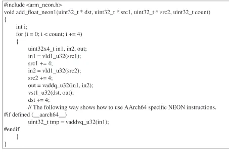
NEON intrinsic code of the addition of array is shown in Figure4.5. Most of the calls in intrinsic NEON code converted to neon assembly instructions using compiler. All the intrinsic methods, such as vld1_u32, are defined in “neon.h”. In the given example, inside the for
loop first individual elements are being load in varialbes and then we add them and finally store in the output register using vst1_u32() method. We have to set the compiler flags as “-mfloat-abi=hard -mfpu=neon” to use floating-point unit (FPU) implementation in the NEON SIMD architecture extension. We should also use compiler option “ -ffast-math -O3” as strict conformance to the floating-point standard (IEEE 754) should be avoided since NEON may not implement it entirely. Compiler can check the flag as __aarch64__ for aarch64 architecture specific instructions.
4.3.2
NEON Assembly
4.3 ARMv7/v8 NEON programming basics 43
#include <arm_neon.h>
void add_float_neon1(uint32_t * dst, uint32_t * src1, uint32_t * src2, uint32_t count) {
int i;
for (i = 0; i < count; i += 4) {
uint32x4_t in1, in2, out; in1 = vld1_u32(src1); src1 += 4;
in2 = vld1_u32(src2); src2 += 4;
out = vaddq_u32(in1, in2); vst1_u32(dst, out);
dst += 4;
// The following way shows how to use AArch64 specific NEON instructions. #if defined (__aarch64__)
uint32_t tmp = vaddvq_u32(in1); #endif
[image:51.595.70.523.258.560.2]} }
.text
.syntax unified .align 4
.global add_float_neon2
.type add_float_neon2, %function .thumb
.thumb_func add_float_neon2: .L_loop:
[image:52.595.75.527.100.340.2]vld1.32 {q0}, [r1]! vld1.32 {q1}, [r2]! vadd.u32 q0, q0, q1 subs r3, r3, #4 vst1.32 {q0}, [r0]! bgt .L_loop bx lr
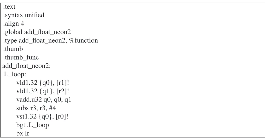
Figure 4.6: Assembly code in .S file for ARMv7.
NEON assembly code uses less instructions to perform the same computations. vld1.32 loads 128-bits from input argument and store in a vector register then vadd.u32 instruction adds two 128-bit vectors and store in third register. Finally the result is being stored in output register using vst1.32 instruction.
[image:52.595.74.527.103.339.2]4.3 ARMv7/v8 NEON programming basics 45
.text .align 4
.global add_float_neon2
.type add_float_neon2, %function add_float_neon2:
.L_loop:
ld1{v0.4s}, [x1], #16 ld1 {v1.4s}, [x2], #16 uqadd v0.4s, v0.4s, v1.4s subs x3, x3, #4
st1 {v0.4s}, [x0], #16 bgt .L_loop
ret
Chapter 5
Field Level Optimizations
1
There is only one NEON based implementation available for pairings in literature. Ana Helena Sánchez et al. [19] tried to use NEON engine to optimize timing for pairing computations on ARM processor based architecture. Ana Helena Sánchez et al. implementation is fastest for 256-bit but there is no implementation for 446-bit and 638-bit security level using NEON engine.
Finite Field multiplier is the most important computation for pairing algorithms. There are many implementations of different scalar multipliers using NEON in literature which can be used to make pairing computation faster on low resource based architectures. Seo and Liu [22] presented modified version of Montgomery multiplier using NEON which is faster than original implementation of Montgomery multiplier. Revisited Montgomery multiplier imple-mentation is effective for 256-bit (8 words), 512-bit (16 words), 1024-bit (32 words) and so on as it uses 4 words in processing simultaniously. This implementaton is not effective for 446-bit (14 words) and 638-bit (20 words) fields and for this reason we use NEON implementation of Schoolbook method.
Seo and Liu [43] presented another multiplier additive Karatsuba Multiplier using ARM-NEON which is an improved version of original Karatsuba multiplier. Additive Karatsuba multiplier is presented as efficient for higher field size multiplications. In the given implemen-tation the Karatsuba method is being used as two level multiplier and montgomery multiplier is being used as the n2–bit multiplications. 446-bit and 638-bit security levels uses odd numbers of byte multiplication so montgomery multiplier for n2–bit multiplication would not be effi-cient. Comba multiplier is very flexible for variable size multiplication which makes it better choice to implement additive Kratsuba multiplier. Our implementation uses Comba multiplier for n2–bit multiplication and compare the implementation result with other multipliers present
in literature.
In this chapter, we present previous efforts made in optimization of the pairing based protocols and our optimization in basic algorithms such as, multiplication, inversion, square.
5.1
Challenges in implementing pairing for higher fields
The concept of Lazy reduction [16] is conveniently implementaed with irreducible binomials in [37]. Aranha et al. [37] proposed efiicient basic computation algorithms e.g., inversion, squaring etc., using lazy reduction and tower asFq→Fq2 →Fq6 →Fq12. According to the
Miller loop implementation explained in [12], for point arithmetic and line evaluation, reduc-tions can be delayed from underlyingFq2field during squaring and multiplication. However,
the upper layer reductions should only be delayed in cases where the technique leads for fewer reductions. In our implementations of lazy reduction most of the reductions are being delayed tillFq2 level. Fq2 reductions are twoFq field reductions and it is efficient to implementFq2
reduction using NEON. We have implemented parallel reduction technique using NEON en-gine inFq2 field which is being used as basic unit forFq6 andFq12reductions and we have used
assembly implementation of Montgomery reduction from relic toolkit [44].
Single precision operations are defined as operands occupying n=⌈⌈log2q⌉/w⌉ words, where w is the word size of machine and double precision operations are defined as with operands of 2nwords. Pairing computations uses both single precision and double precision operations accordingly in tower computations. Lazy reduction technique is effective for up-per layer algorithm up-performance, but there are some penalties for the use of lazy reduction technique. With lazy reduction technique, reduction is being delayed till lower layers which replace single precision operations in higher field with double precision operations. For higher security levels, when prime field size is larger than the word size and there are less number of registers to hold the data (e.g., ARM has 12 general purpose registers) longer computations loading data from memory could slowdown the overall performance. This is the reason that single and double precision algorithms should be optimized for systems with low resources. However, this disadvantage can be minimized up-to some extend using NEON engine as extra SIMD registers can be used for parallel load/store and computations which leads to improve performance of basic algorithms.
5.2 Proposed NEON implementation of Schoolbook multiplier. 49
Algorithm 5.1Parallel multiplication(mulN)using NEON [19]
Inputs:a= (a0,a1),b= (b0,b1),c= (c0,c1)andd= (d0,d1) a,b,c,d∈FqOutput:M=a.bandN=c.d
1:M←0,N←0 2:fori=0→1do
3: T1←0,T2←0
4: for j=0→1do
5: (T1,C1)←Mi+i+aj.bi+T1,(T2,C2)←Ni+i+cj.di+T2
6: Mi+j=C1,Ni+j=C2
7: end for
8: Mi+n=T1,Ni+n=T2
9: return(M,N)
10: end for
5.2
Proposed NEON implementation of Schoolbook
multi-plier.
For this work, we have implemented Schoolbook multiplier using NEON for BN-446 and BN-638 curves. The algorithm uses NEON implementation of Montgomery multiplier as described in [19] and described in Algorithm5.1for half size multiplication. Algorithm5.1, represnts the base multiplier. The input arguments are four numbersa,b,c,d and outputs are
M=a.bandN=c.das the product of two input arguments. We are referencing algorithm5.1
asmulN in rest of the paper and the steps are as follows:
• The step-1 of Algorithm5.1initialize the output variable as zero.
• Two loops as shown in step 2 and step-4 of Algorithm 5.1 iterate over the two input arguments.T1andT2are variables to hold temporary values.
• Step-5 performs the parallel multiplication and assign the values forC1andC2as carries
for each step to further values ofM andN. After for loop of step-4 ends, T andT2are
assigned to second half of the output valuesMandN.
• Finally, at the end of both for loops the output will be products of 4 numbers, stored in two numbers.
Step-1 : Parallel Multiplication using NEON
Step-3: Addition using ARM assembly. Step-2 : Parallel Multiplication
using NEON Inputs arguments, A and B
Output
NEON implementation of Schoolbook multiplier
n
1
A A0
1 1 B Au A 2 n n 1
B B0
B 2 n 2 n 2 n 0 0 B A u n n 1 0 B Au 0 1 B Au n n 1 1 B
Au A0uB0
[image:58.595.108.456.118.396.2]n 2 C 1 0 B A u 0 1 B A u 2 n 2 n 2 n 2 n
Figure 5.1: Graphic interpretation of Schoolbook Multiply Algorithm using NEON.
numbers using NEON. Step-3 is threen−bitnumber addition using ARM assembly. NEON is not effective for additions because of carry handling so the step-3 is being implemented in ARM assembly. Finally the output C is 2n-bit long number.
We also have used Coarsely Integrated Operand Scanning (CIOS) for parallel Fq2 field
multiplication as explained in [19] and using its reference asmulRedN in rest of the paper.
5.3
Karatsuba multiplier using NEON
Karatsuba multiplier is defined in Equation3.2. In this work, we have implemented the Ad-ditive version of Karatsuba multiplier. As described in Algorithm5.3, the inputs for Additive Karatsuba algorithm aren–bit numbersa= (a0,a1),a∈Fqandb= (b0,b1),b∈Fqand output
is 2n–bit numberC=a.b. The steps are defined as:
• Step-1 calculates the parallel multiplication of (a0,b0)and(a1,b1)and store the result
5.3 Karatsuba multiplier using NEON 51
Algorithm 5.2Schoolbook Multiplier using NEON
Inputs:a= (a0,a1),a∈Fq
b= (b0,b1),b∈Fq
Output:C=a.b
1:(M0,N0)←mulN(a0,b0,a1,b1)
2:(M1,N1)←mulN(a0,b1,a1,b0)
3:C=N0.2n+M0
4:C=C+M1.2
n
2
5:C=C+N1.2
n
2
6: returnC
Algorithm 5.3Karatsuba Multiplier using NEON
Inputs:a= (a0,a1),a∈Fq
b= (b0,b1),b∈Fq
Output:C=a.b
1:(M,N)←mulN(a0,b0,a1,b1)
2:(AC,AS) =a0+a1
3:(BC,BS) =b0+b1
4:S=AS.BS
5:S=S+ (AND(COM(AC),BS)).2
n
2
6:S=S+ (AND(COM(BC),AS)).2
n
2
7:S=S+ (AND(AC,BC)).2
n
2
8:C=N.2n+ (S−M−N)2n2+M
9: returnC
• Step-2 and step-3 calculate the sum(A)of then2–bit of each numbers and store the carry and sum in separate variables.
• Step-4 calculates the product(S)of result of each step-2 and step-3.
• Step-5 and step-6 performs the addition of result of step-4 with carry handler. COM function is the 2’s compliment of the input.AND(COM(AC),BS),AND(COM(BC),AS)
and(AND(AC,BC))are being added to adjust the carry from previous steps.
Algorithm 5.4Squaring overFq2 [19]
Inputs:M=m0+m1i; m0,m1∈Fq;
Output:N=M2 ∈ Fq2
1:N0←m0−m1
2:t←m0+m1
3:(n1,n0)←mulN(m0,m1,N0,t)
4:n1←2n1
5:n0←n0−n1
6:returnN=n0+n1i
5.4
Reduction using NEON
Modular multiplication is the one of the most important base field arithmetic in pairing com-putations. Montgomery multiplication method is effective for reduction step. Algorithm3.7
explains the classic reduction method and w