Singularities of Optimal Control Problems on some
Six Dimensional Lie groups
James Biggs, William Holderbaum, and Velimir Jurdjevic
Abstract— This paper considers the motion planning prob-lem for oriented vehicles travelling at unit speed in a three-dimensional space. A Lie group formulation arises naturally and the vehicles are modelled as kinematic control systems with drift defined on the orthonormal frame bundles of particular Riemannian manifolds, specifically the three-dimensional space forms Euclidean spaceE3
, the sphereS3
and the hyperboloidH3 . The corresponding frame bundles are equal to the Euclidean group of motions SE(3), the rotation group SO(4) and the Lorentz group SO(1,3). The Maximum Principle of optimal control, shifts the emphasis for these systems to the associated Hamiltonian formalism. For an integrable case the extremal curves are explicitly expressed in terms of elliptic functions. In this paper, a study at the singularities of the extremal curves are given, which correspond to critical points of these elliptic functions. The extremal curves are characterized as the intersections of invariant surfaces and are illustrated graphically at the singular points. It is then shown that the projections of the extremals onto the base space, called elastica, at these singular points, are curves of constant curvature and torsion, which in turn implies that the oriented vehicles trace helices.
Index Terms— Optimal Control, Lie Groups, Integrable Hamil-tonian Systems, Singularities.
I. INTRODUCTION
This paper is motivated by the problem of motion planning for oriented vehicles moving with unit speed in a three-dimensional space, such as the airplane landing problem [1]. For such problems the orientation of the vehicle is naturally represented by an orthonormal frame over a point in the underlying manifold, that is, the configuration space of the vehicle can be taken as the orthonormal frame bundle of the manifold, and the motions of the vehicle are described by curves in this bundle. In this paper we consider three-dimensional spaces for which the orthonormal frame bundle coincides with the isometry group. They are, the Euclidean space E3, the sphere S3 and the hyperboloid H3. The corresponding isometry groups are the Euclidean group of motion SE(3), the rotation group SO(4) and the Lorentzian group SO(1,3). The Euclidean setting has been used to study multi-vehicle formation control of Unmanned air vehicles [2], the airplane landing problem [1] and the control of underactuated Underwater Vehicles [3]. In each of these cases the oriented vehicles trace paths in E3. In this paper we generalize the Euclidean frame, simultaneously
J. Biggs is with School of Systems Engineering, University of Reading,
Reading, United [email protected]
W. Holderbaum is with School of Systems Engineering, University of
Reading, Reading, United [email protected]
V. Jurdjevic is with the Department of Mathematics, University of Toronto,
Toronto, [email protected]
studying oriented vehicles in the space formsE3,S3 andH3, as in [4].
In [2] the authors use the Euclidean Serret-Frenet Frame to model Unmanned Air vehicles as particles moving at unit speed in Euclidean space, where the controls take the form of the geometric invariants curvature and torsion. In addition [5] uses a generalized Serret-Frenet frame adapted to curved spaces to describe the motion of relativistic particles in S3 and H3. For a description of the Serret-Frenet frame and its formulation on Lie groups, see [6]. Although the Serret-Frame is adequate in describing the motions of particles it is inadequate in describing oriented bodies.
More general Euclidean frames have been used to describe the motion of underwater vehicles in [3] and airplanes in [1]. In this work we use the most general orthonormal frames to simultaneously study the motion planning problem for oriented vehicles travelling in E3,S3 andH3. For a detailed description of space forms, their frame bundles and their tangent spaces see [7].
The motion planning problem for oriented vehicles has been tackled using local representations of Lie groups i.e. the Wei-Norman representation and Magnus representation to describe the behavior of such systems and then classical methods from nonlinear control e.g. averaging on Rn have
been adapted to these coordinate representations, see [8]. However, because in general these representations are local, only small reorientations can be performed at any one time and highlights the need for global methods to plan larger, more energy efficient manoeuvres.
The application of the Maximum Principle of optimal control shifts the emphasis to the language of symplectic geometry and to the associated Hamiltonian formalism. The Maximum principle states that the optimal solutions are the projections of the extremal curves onto the base manifold, where the extremal curves are solutions of certain Hamiltonian systems on the cotangent bundle T∗G. As the base manifolds of the oriented vehicle is a Lie group G, the cotangent bundle T∗G can be realized as the direct product G×g∗ where
g∗ is the dual of the Lie algebra g of G. Therefore, the original Hamiltonian defined on T∗G can be written as a reduced Hamiltonian on the dual of the Lie algebra g∗. The corresponding Hamiltonian vector fields are then expressed in non-canonical form and will be referred to as the reduced Hamiltonian vector fields.
For a symmetric oriented vehicle, where two moments of inertia c2 andc3 are equal, the Hamiltonian vector fields are
integrable (see [13] for a detailed description of integrable Hamiltonian systems on Lie groups) and we derive explicit expressions for the extremal curves. For integrable systems their topological and qualitative properties such as bifurcations and singularities are of great importance and knowledge about these properties will give us some information about the dynamical properties of a perturbed Hamiltonian or near integrable Hamiltonian, as outlined in [14].
For the reduced integrable Hamiltonian system the extremal curves are explicitly expressed by elliptic functions. Using these explicit expressions we investigate the singularities of the Hamiltonian vector fields. The singularities, or singular points, are equilibria for the reduced Hamiltonian system and are defined at the roots of the cubic function that appear in the explicit expression of the extremal curves. The singularities of the reduced Hamiltonian are important in the motion control of vehicles as they coincide with relative equilibria for the original Hamiltonian system. Indeed, it is shown that the projections of the extremal curves at a singularity onto the base space are helical curves. This implies that the extremal controls at a singularity induce steady motions of the vehicle i.e. constant translation and/or constant rotation. Once these relative equilibria have been identified such techniques for stabilization and control can be used as in [8]. Studying these systems and their singularities provide insight into the rich qualitative and topological nature inherent in the motion planning of vehicles.
In this paper the motions of oriented vehicles are restricted to move at unit speed. Under this restriction the motion planning problem of steering the vehicle from an initial configuration to a final configuration, in a fixed time, while minimizing the amount of manoeuvering the vehicle will do, can be equated to the elastic rod problem of Kirchhoff, which is detailed in [13]. In the elastic problem the projections of the extremal curves onto the base space, called elastic curves, reflect the shape of an elastic rod, of fixed length, forced to have some initial and final position and orientation. Therefore, in this motion planning problem, the oriented vehicles will trace elastic curves. In the Euclidean case, Kirchhoff elastic rods have been used to model practical problems such as the dynamic formation of DNA and to explain the looping of
marine cables, see [15].
The original contributions in this paper are summarized in the following statement:
II. STATEMENT OFCONTRIBUTIONS
• The extremals are explicitly expressed in terms of cubic curves which are parameterized by elliptic functions. • The curvature and torsion of the elastic curves are
ex-plicitly expressed by elliptic functions.
• The critical points of this cubic correspond to periodic extremal curves characterized as the intersections of invariant surfaces, which are illustrated graphically. • The elastic curves at the singularity are shown to be of
constant curvature and constant torsion and therefore the oriented vehicles trace helices.
III. EXTREMAL CURVES INse(3)∗,s0(4)∗ANDs0(1,3)∗
In this section we will state the elastic problem and equate it to the motion planning problem for oriented vehicles moving with unit speed in a three-dimensional space. Firstly, the group G is used to represent the frame bundle of the space forms. The analysis here is restricted to the three dimensional space forms and therefore the corresponding frame bundles are the matrix Lie groupsSE(3), SO(4)and SO(1,3). We identify T G with G×g where g is the Lie algebra of G via the left translations. The elastic problem on the three dimensional space forms concerns the solutions g(t) ∈ G of the left-invariant differential system:
dg
dt(t) =g(t)(B1+
3
X
i=1
uiAi)
=g(t)
0 −ε 0 0
1 0 −u3 u2
0 u3 0 −u1
0 −u2 u1 0
(1)
that minimize the expression
1 2
Z T
0
(u(t), Qu(t))dt (2)
subject to the given boundary conditiong(0) =g0,g(T) =g1.
g(t)∈GwhereGdepends onεand isSE(3)forε=0,SO(4)
for ε=1 and SO(1,3) for ε=-1, so we are simultaneously studying all three cases. B1, A1..., A3 are given matrices in
the Lie algebra gof G, the ui’s play the role of the control
functions and Q is a positive definite 3 ×3 matrix. This problem can be identified with the elastic rod problem of Kirchhoff, by replacing timet with the arc length parameter of the curve s and in the expression (2) the terminal time T should be replaced with the length of the rod l. Then γ(s) corresponds to the central line of the rod. The physical characteristics of the rod, related to the geometric shape of its cross section are reflected in the constants, callci, dependent
space form M. It follows that the problem of minimizing the expression (2) is equivalent to minimizing locally the amount of bending and twisting in the rod.
Proceeding to equate the elastic problem to the problem of motion planning of a vehicle, the principal moments of inertia ci of the vehicle are dependent on the matrix Q and the
controls ui relate to the angular velocity of the vehicle. It
follows that (1) describe the kinematic equations of the vehicle such that the vehicle traces out a trajectory γ(t)∈M which are related to g(t) ∈ G via the projection γ(t) = g(t)~e1
where~e1 is a basis element in a standard orthonormal frame
~e1, ~e2, ~e3, ~e4∈R4. The projected curvesγ(t)∈M are called
elastic curves, where M =E3 when g(t)∈SE(3),M =S3 when g(t) ∈ SO(4) and M = H3 when g(t) ∈ SO(1,3). It follows from (1) that the vehicle is restricted to travel at unit speed
° ° °
dγ(t)
dt ° °
° = 1 and in addition dγ(t)
dt coincides with
the first leg of the frame (see [7] for detail). The solutions g(t)∈Gof (1) while minimizing the expression (2) are locally optimal, that is optimal for small terminal timeT, however as the terminal time grows they may stop being optimal. For simplicity of terminology we will refer to all projections as the optimal solutions even though the nature of cut-locus and conjugate points have not been considered, see [6]. Minimizing the cost function (2) is then equivalent to minimizing the control energy of the vehicle between an initial position and orientation and a final position and orientation.
The Maximum Principle of optimal control identifies the appropriate left-invariant Hamiltonian H on the dual of the Lie algebrag∗, (see [6]). The Maximum Principle, as a general necessary condition of optimality, leads to the appropriate Hamiltonian on the cotangent bundle of the Lie Group G, hence the extremal curves belong toT∗G. Then the Maximum Principle considers the lift of the optimization problem to the cotangent manifold T∗G. The control Hamiltonian is written as:
H(p, u) =p(gB1) + 3
X
i=1
uip(gAi)−p0(1
2
3
X
i=1
ciu2i) (3)
where p ∈ T∗
gG and p0 > 0 is a fixed positive constant
andH(p, u)is a concave function with respect toui. It then
follows from the Maximum Principle that the extremal control functionsu∗
i are determined from the condition:
dH dui
= 0
differentiating (3) with respect to ui gives
dH dui
=p(gAi)−ciui
where i= 1,2,3. Therefore, the extremal controls are given in feedback form:
u∗
i =
1
ci
p(gAi)
where i = 1,2,3. Because of the non-holonomic nature of these problems, the extremal curves that correspond to an optimal trajectory can be either abnormal or normal i.e. there are two types of Hamiltonian to consider. p0 is set to 1 for
normal extremals and 0 for abnormal extremals. All of these
problems admit abnormal extremals, however, because of the regularity of these variational problems each optimal trajectory is a projection of a regular extremal curve. Therefore, assume p0= 1 to consider only regular extremals.
The Hamiltonian for such systems are functions on the cotan-gent bundleT∗Gwhich can be trivialized from the left such that T∗G=G×g∗. Therefore, the appropriate Hamiltonian is a function on g∗ the dual of the Lie algebra gof G. The Hamiltonian (3) can be pulled back by the left or right. The pull-back in this case is explicitly stated asp(·) = ˆp(g−1(·)). i.e p∈ T∗G is pulled back to give a function pˆ ∈ g∗. The control Hamiltonian can then be written as
H(ˆp, u) = ˆp(B1) + 3
X
i=1
uipˆ(Ai)−
1 2
3
X
i=1
ciu2i (4)
This Hamiltonian is a function of the controls only, and so it does not depend explicitly on elements in G. In other words it is left invariant in that it does not change by the group multiplication on the left. In addition, define the extremal curves pi = ˆp(Bi) andMi = ˆp(Ai) then it follows that the
extremal controls can be expressed as
u∗
i =
1
ci
Mi (5)
it follows from the formula (5) that the extremals Mi
corre-spond to components of angular momentum. Substituting these back into (4) gives the optimal Hamiltonian
H∗=p
1+
1 2
µM2 1
c1 +
M2 2
c2 +
M2 3
c3
(6)
the extremal control functionsui∗ are additionally substituted
into (1) to yield
g−1dg dt =
0 −ε 0 0
1 0 −M3/c3 M2/c2
0 M3/c3 0 −M1/c1
0 −M2/c2 M1/c1 0
(7)
To proceed it is essential to recognize some geometric facts about these Lie algebras. The variational problem on Lie groups in this paper are associated with the Cartan decom-position ofgof a Lie groupGinto the factorsp andkwhich satisfy the classic relations
[k,k]⊆k,[p,k]⊆p and[p,p]⊆k
wherekconsists of all matrices of the form
0 0 0 0
0 0 −α3 α2
0 α3 0 −α1
0 −α2 α1 0
andpconsists of the matrices
0 −εb1 −εb2 −εb3
b1 0 0 0
b2 0 0 0
b3 0 0 0
The corresponding basis elements for kandpare:
A1=
0 0 0 0 0 0 0 0 0 0 0 −1 0 0 1 0
, A2=
0 0 0 0 0 0 0 1 0 0 0 0 0 −1 0 0
A3=
0 0 0 0 0 0 −1 0 0 1 0 0 0 0 0 0
, B1=
0 −ε 0 0 1 0 0 0 0 0 0 0 0 0 0 0
B2=
0 0 −ε 0 0 0 0 0 1 0 0 0 0 0 0 0
, B3=
0 0 0 −ε
0 0 0 0 0 0 0 0 1 0 0 0
A1, A2, A3, B1, B2, B3 describe infinitesimal motion in the
roll, pitch, yaw, surge, sway and heave directions of the vehicle respectively. The Lie bracket is defined as[X, Y] =XY−Y X and the corresponding Lie bracket table is then:
[,] A1 A2 A3 B1 B2 B3
A1 0 A3 -A2 0 B3 -B2
A2 -A3 0 A1 -B3 0 B1
A3 A2 -A1 0 B2 -B1 0
B1 0 B3 -B2 0 εA3 -εA2
B2 -B3 0 B1 -εA3 0 εA1
B3 B2 -B1 0 εA2 -εA1 0
Using the optimal Hamiltonian (6), it is possible to construct the corresponding Hamiltonian vector fields XH∗ using the
Poisson bracket defined on the symplectic manifold. The Hamiltonian vector fields are calculated using the formula XH∗[·] = {·, H∗} where the Poisson bracket is associated
with the Lie bracket by{Mi, Mj}=−pˆ([Ai, Aj]). Therefore,
it follows that:
dM1
dt ={M1, H
∗}={M
1, p1}+M1
c1
{M1, M1}
+M2
c2
{M1, M2}+
M3
c3
{M1, M3}
= 0 + 0− 1 c2
M2M3+ 1
c3
M3M2
= c2−c3
c2c3 M2M3
the remaining derivations of the Hamiltonian vector fields are left to the reader and yield:
dM1
dt ={M1, H
∗}=−M2M3 c2
+M2M3
c3
dM2
dt ={M2, H
∗}=M1M3 c1 −
M1M3
c3 +p3
dM3
dt ={M3, H
∗}=−M1M2 c1
+M1M2
c2
−p2
dp1
dt ={p1, H
∗}= −M2p3 c2
+p2M3
c3
dp2
dt ={p2, H
∗}= M1p3 c1
−p1M3 c3
+εM3
dp3
dt ={p3, H
∗}=−M1p2 c1
+p1M2
c2
−εM2
(8)
In this paper the analysis is restricted to an integrable case of the Hamiltonian vector fieldsXH∗. Explicitly a Hamiltonian
function on a symplectic manifoldN of dimension 2nis said to be integrable if there exist functions ϕ2, ..., ϕn on N that
together with the HamiltonianH∗=ϕ
1 satisfy the following
two properties:
• ϕ1, ..., ϕn are functionally independent i.e the
differen-tials dϕ1, ..., dϕn are linearly independent for an open
subset ofN.
• The functionsϕ1, ..., ϕn are in involution.
Thus, in identifying the (n−1)functionsϕi and the
Hamil-tonian function the system is completely integrable. In the mechanics literature these are called integrals of motion. The Casimir functions are constant on co-adjoint orbits ofG, and are integrals of motion for any left-invariant HamiltonianH∗. There are also two extra integrals of motion corresponding to their right-invariant Hamiltonian. They are in involution with each other, and also in involution with H∗ and the two Casimir functions. Hence, altogether they account for five independent integrals of motion and the system becomes completely integrable whenever there is just one more integral of motion. For left-invariant control systems defined on semi-simple Lie algebras, the Casimir functions are derived through the invariance of the Killing form. In the case of SE(3) the Killing form is degenerate and therefore the Casimir functions are derived in a different way (see [7] for a detailed description of their derivation), explicitly the Hamiltonian and Casimir functions are:
H∗=p
1+ 1 2( M2 1 c1 +M 2 2 c2 +M 2 3 c3 ) (9)
I2=p21+p22+p23+ε(M12+M22+M32) (10)
I3=p1M1+p2M2+p3M3 (11)
An extra integral of motion exists in a case analogous to Lagrange’s top [16]. Proceeding by equating c2 = c3 and
normalizing the constants such that c2 = c3 = 1, and
c1 6= 0, yields an extra integral of motion required for
Liouville integrability, see [16] for a description. The condition c2=c3= 1 in (8) gives:
dM1
dt = 0
and therefore M1 is a constant of motion which will be
denoted σ, the Hamiltonian vector fields (8) reduce to:
dM2 dt = σM3 c1
−σM3+p3
dM3
dt = −σM2
c1
+σM2−p2
dp1
dt =−M2p3+p2M3 dp2
dt = σp3
c1
−p1M3+εM3
dp3
dt =− σp2
c1
+p1M2−εM2
In a similar manner to [1], we proceed to solve for the extremal control functions:
dp1
dt =p2M3−M2p3 it follows that
(dp1
dt )
2=p2
2M32+p23M22−2p2p3M2M3 (13)
Using (9) and (10) write;
2(H∗−p
1)−
σ2
c1
=M2 2 +M32
I2−p21−ε(σ2) =p22+p23+ε(M22+M32)
(14)
multiplying the two equations in (14) gives:
(I2−p21−ε(σ2))(2(H∗−p1)−σ 2
c1
) =
p22M22+p22M32+p23M22+p23M32+ε((M22+M32)2)
(15)
To find explicit solutions it is necessary to use the Casimir function (11)
I3−p1σ=p2M2+p3M3 (16)
squaring (16) yields:
(I3−p1σ)2=p22M22+p23M32+ 2p2M2p3M3 (17)
Therefore, substituting (17) and (15) into (13) gives the following cubic function:
f(p1) = (
dp1
dt )
2= (I
2−p21−ε(σ2))(2(H∗−p1)−
σ2
c1
)
−(I3−p1σ)2−ε((2H∗−
σ2
c1
−2p1)2)
(18) The function f(p1)is then a cubic function of p1 and
deter-mines the qualitative behavior of an arbitrary elastic curve. The solutions are therefore given in terms of elliptic functions, as demonstrated in subsection III-A.M2andM3can be solved in
terms of p1 and the constants of motion. Proceeding to solve
the extremals and using the Hamiltonian function (9) where M1 is a constantσ, the reduced Hamiltonian is
M22+M32= 2(H∗−p1)−
σ2
c1
(19)
This suggests using polar coordinates forM2 andM3;
θ(t) = arctan µ
M2
M3
(20)
˙
θ= M3M˙2−M2M˙3
M2 2 +M32
substituting in the values forM˙2 andM˙3 from (12) gives
˙
θ=M3 ³
M1M3
c1 −M1M3+p3 ´
M2 2 +M32
+
M2
³
−M1M2
c1 +M1M2−p2 ´
M2 2 +M32
and on simplifying can be expressed as:
˙
θ= σ
c1
−σ+ I3−p1σ 2(H∗−p1)−σ2
c1
(21)
It is easy to solve explicitly for the radius from (19)
r(t) = s
2(H∗−p1)−σ
2
c1
(22)
Therefore, the extremal control functions are
u∗
1=
M1(t)
c1
= σ
c1
u∗
2=M2(t) =r(t) sin(θ(t))
u∗
3=M3(t) =r(t) cos(θ(t))
(23)
Note that θ(t) is analogous to the nutation angle for the Lagrange top (see [16]). The extremals are therefore only dependent on the constants of motion andp1.
A. Explicit solution ofp1
For the purpose of this paper the critical points of the cubic function (18) are of importance. However, we show here that (18) can be solved in terms of a Weierstrass’ ℘-function, a meromorphic function of complex time z. The equations for p1 will be converted into the canonical equation for the
Weierstrass’ ℘-function (see [17]):
˙
℘2= 4℘3−g2℘−g3 (24)
where g2 andg3 are the elliptic invariants to be determined
and that specify℘completely. The Weierstrass’℘function is often denoted℘(z;g2, g3), where z∈C. In this problem z is
time and therefore we restrict ourselves to the real values ofz, then ℘(z;g2, g3) is real. The equation (18) can be converted
into this canonical form via an affine input transformation:
p1=a℘+b (25)
whereaandbare constants and therefore
˙
p1=a℘˙ (26)
Although the equation (18) can be solved for any constant c1, we assume c1 = 1 for simplicity of this illustration.
Substituting (25) and (26) into (18) gives:
a2℘˙2= 2a3℘3
+2a2(3b−2ε−H∗)℘2
+2a(3b2+ 4εH∗−2b(2ε+H∗)−I
2+I3σ−εσ2)℘
+2b3−4εH∗2−2b2(2ε+H∗) + 2H∗I
2
−I2
3+ 2εH∗σ2−I2σ2+ 2b(4εH∗−I2+I3σ−εσ2)
(27) Comparing the coefficients of equation (27) to (24) and simplifying we obtain:
a= 2
b=2ε+H ∗
Therefore, p1 can be expressed explicitly as a Weierstrass’
℘-function under the affine transformation:
p1= 2℘(z;g2, g3) +
2ε+H∗ 3
Consequently p1 is a meromorphic function and the elliptic
invariants are:
g2=
1 3(4ε
2−8εH∗+H∗2+ 3I
2−3I3σ+ 3εσ2)
and
g3=
1 108(32ε
3+ 4H∗3−18H∗(2I
2+I3σ)
+ε2(−96H∗+ 36σ2) +12ε(5H∗2+ 3I
2−3I3σ−3H∗σ2) + 27(I32+I2σ2))
These calculations demonstrate that the integration procedure is essentially the same for all three space forms with the solutions only differing by the parameter ε = 1,−1,0. In addition it is shown in [17] that the discriminant of the cubic
4℘3−g
2℘−g3= 0is
∆ =g23−27g23 (28)
and ifg2andg3 are real then the cubic4℘3−g2℘−g3= 0,
determines the qualitative nature of the solutions where the cubic has:
• three distinct real roots if ∆>0.
• three real roots which are not all distinct if ∆ = 0.
• a real root and a pair of complex conjugate roots if∆< 0.
IV. THESERRET-FRENETFRAME:CURVATURE AND TORSION OF ELASTICA
In order to draw geometric conclusions in terms of curvature and torsion of the corresponding elastic curves it is necessary to relate the extremals which have been solved to the curvature κand the torsionτ along the central line. Therefore, it is nec-essary to relate the differential equation (1) to the differential equation expressed in terms of curvature and torsion, called the Serret-Frenet frame:
d¯g(t)
dt = ¯g(t)
0 −ε 0 0 1 0 −κ 0 0 κ 0 −τ
0 0 τ 0
(29)
where g¯(t) ∈ G. Denote the standard basis elements of a vector in R4 as ~e1, ~e2, ~e3, ~e4 withg¯(t)~e1 =γ(t) whereγ(t) is a curve in the manifold M, then the tangent vector T~ = ¯
g(t)~e2, the normal vectorN~ = ¯g(t)~e3and the binormal vector
~
B = ¯g(t)~e4. Therefore differentiating T~ and substituting in
equation (29) gives:
d ~T dt =
dg¯
dt~e2= ¯g(t)
0 −ε 0 0 1 0 −κ 0 0 κ 0 −τ
0 0 τ 0
~e2
= ¯g(t)(−ε~e1+κ~e3) =−εγ(t) +κ ~N
(30)
and in the same manner as (30) obtain the differential equa-tions describing the Serret-Frenet Frame:
d ~N
dt =−κ ~T +τ ~B d ~B
dt =−τ ~N
(31)
Let ~a1, ~a2, ~a3 be an orthonormal frame fixed at a point on
the body, called themoving frame. The Serret-Frenet Frame is shown to be explicitly related to the moving frame in [6]. Here we proceed to solve for the curvature and torsion of the elastic curves in terms of the meromorphic function p1 and
the constants of motion (9), (10), (11).
In these cases the Serret-Frenet frame and the elastic (general) frame are adapted to the curve γ(t) in such a way that the first leg of the frame coincides with the tangent of the curve
dγ(t)
dt =~a1=T~ implies that~a2and~a3are in the normal plane
spanned byN~ andB. Define an angle~ β that the normalN~ makes with~a2 then:
~
N = (cosβ)~a2+ (sinβ)~a3
~
B= (−sinβ)~a2+ (cosβ)~a3
(32)
Differentiating N~ gives
d ~N dt =
dβ
dt((−sinβ)~a2+(cosβ)~a3)+(cosβ) d~a2
dt +(sinβ) d~a3
dt (33) Let R∈ SO(3) be the matrix that relates coordinates in the moving frame to coordinates in the fixed frame along γ(t), explicitly ~ai = R~ei. In addition as the tangent space at R
can be either a left or right translation at the identity then
dR
dt =A(u)R whereA(u)∈krelates to the controlled vector
fields (the horizontal vectors in the Cartan decomposition) in our problem:
A(u) =
0 −u3 u2
u3 0 −u1
−u2 u1 0
andω(t)is used to denote its corresponding coordinate vector related byA(u)x=x×ω(t)for allx∈R3 where
ω(t) =
u1
u2
u3
then
d~ai
dt = dR
dt~ei=A(u)R~ei
=A(u)~ai=~ai×ω(t)
(34)
from (34) and writing~ai in its standard basis we can obtain
two useful equations:
d~a2
dt =−u3~a1+u1~a3 d~a3
dt =u2~a1−u1~a2
substituting (35) into (33) and rearranging gives the following expression:
d ~N
dt = ((−cosβ)u3+ (sinβ)u2)~a1 −
µ
dβ
dt sinβ+u1sinβ
~a2
+ µdβ
dt cosβ+u1cosβ
~a3
(36)
Using the equation d ~dtN =−κ ~T+τ ~B from (31) and substitut-ing in the expressions for T~ andB~ gives:
d ~N
dt =−κ~a1+τ((−sinβ)~a2+ (cosβ)~a3) (37) Identifying (36) with (37) yields:
κ=u3cosβ−u2sinβ
τ= dβ
dt +u1
(38)
To obtain a direct relation between the extremals and torsion it is necessary to obtain an expression for β in terms of the controls. DifferentiatingB~ in (32) gives:
d ~B dt =
dβ
dt ((−cosβ)~a2+ (−sinβ)~a3)
+(−sinβ)d~a2
dt + (cosβ) d~a3
dt
(39)
Substituting (35) into (39) gives:
d ~B
dt = (u2cosβ+u3sinβ)~a1 −
µ
u1+
dβ dt
(cosβ)~a2−
µ
u1+
dβ dt
(sinβ)~a3
(40)
Substituting N~ from (32) into d ~dtB = −τ ~N from (31) and equating to (40) immediately yields:
u2cosβ+u3sinβ= 0 (41)
Thus the equation for the angle β can be written explicitly in terms of the controls as:
tanβ=−u2 u3
(42)
Summarizing
κ=u3cosβ−u2sinβ
τ= dβ
dt +u1
tanβ=−u2 u3
(43)
In our case the Hamiltonian corresponds toH∗=p
1+12(σ
2
c1+
M2
2+M32)which is generated by the optimal controlsu1(t) =
M1
c1 =
σ
c1 u2(t) =M2andu3(t) =M3, therefore the curvature
can be written explicitly in terms of the extremals. Squaring the equation for the curvature (43) and adding to the square of equation (41) yields:
κ2=u22+u32=M22+M32 (44)
and substituting (9) into (44) gives:
κ2= 2(H∗−p
1)−
σ2
c1
(45)
Here we proceed to solve the torsion in terms of the mero-morphic function for this particular case. From (42) and substituting the extremals gives:
tanβ=−M2 M3
(46)
Differentiating (46) yields:
sec2βdβ dt =
M2M˙3−M3M˙2
M2 3
(47)
substituting in the equations forM˙2 andM˙3 from (12) gives:
sec2βdβ dt =
M2(−Mc11M2 +M1M2−p2)
M2 3
−M3(
M1M3
c1 −M1M3+p3)
M2 3
(48)
In addition using equation (46) to derive sec2β = M 2 2+M
2 3
M2 3
and substituting into (48) gives: dβ
dt =M1(1−
1
c1)−
M2p2+M3p3
M2 2 +M32
(49)
then substituting (49) into the equation for the torsion (43) gives:
τ =−M2p2+M3p3 M2
2 +M32
+M1 (50)
using the constants of motion (16), recalling thatM1=σ in
the integrable case and equation (44), then (50) can be written in terms of the meromorphic functionp1:
τ =−I3−p1σ
κ2 +σ (51)
As the equations (45) and (51) are expressed in terms of the constants of motion and the meromorphic function p1, it is
clear that ifp1 is constant then the curvature and torsion are
also constant. Therefore, at the singularity the elastic curves have constant curvature and constant torsion and are therefore generalized helices. This implies that at the singularities of the cubic function (18) (when dp1
dt = 0), the projections onto
the base space correspond to steady motions i.e. constant translations and/or constant rotations.
V. THE GEOMETRY AT THE SINGULARITIES OF THE
EXTREMAL CURVES
In this section a discussion is given of the equilibria of the reduced Hamiltonian vector fields. From equations (12) it is clear to see that there exists a trivial fixed point in all the cases
(ε=−1,0,1) when p1 =p2 =p3=M1 =M2=M3 = 0.
At these fixed points the corresponding elastic curves are the geodesics. In addition a degeneracy occurs in the Euclidean case corresponding to the level set I2 = 0. This is the case
[1] result from a highly simplified model where helical elastic curves are found under the condition thatI2= 0. In this paper
we study the general case when I2 6= 0. In the general case
there are equilibria of the system that are less obvious and can be seen from the explicit solutions which occur at the roots of the cubicf(p1) = 0 in (18). The equilibria of the reduced
Hamiltonian system corresponding to the roots of this cubic will be called singularities. It is shown here that at the roots of the cubic the extremals define a closed periodic orbit. A geometric interpretation is given in terms of the intersection of invariant surfaces and explicit solutions stated. Here we begin with a brief comment on the level set I2 = 0 before
moving onto the singularities defined at the root of the cubic.
A. The Level set I2= 0
The level set I2 = 0 (equation (10)) in the Euclidean
case is analogous to the Euler top (left-invariant heavy top) in the mechanics literature (see [16]). I2 = 0 when ε = 0
implies that p1 = p2 =p3 = 0for all time. Along with the
assumptionc1=c2=c3 which is the case studied in [1], the
corresponding elastic curves were used to find optimal landing trajectories for airplanes, and where the equations of motion (12) degenerate to:
dM1
dt = 0 dM2
dt = 0 dM3
dt = 0
M1, M2 and M3 are constants of motion and therefore the
optimal controls are constants. In [1] it is shown that the elastic curves corresponding to constant controls ui are helices. In
addition ifM1is zero the elastic curves reduce to Riemannian
circles. If all the controls are zero then the elastic curve are geodesics. In the spherical and hyperbolic case, this particular degeneracy does not occur. In these casesI2= 0corresponds
to p1 = p2 = p3 = M1 = M2 = M3 = 0 for ε = 1
where the elastic curves are geodesics and in the hyperbolic caseε=−1implies that the extremals exist on the light-cone p21+p22+p23 =M12+M22+M32. This case requires further
investigation and is left to future research.
B. Critical points of the cubic functionf(p1)
The explicit solutions of the Hamiltonian vector fields are solely dependent on the constants of motion and the initial conditions of the meromorphic function p1, which
is defined in terms of elliptic functions. The initialization of p1 is therefore essential in determining the qualitative
behavior of the system. To understand the behavior of p1
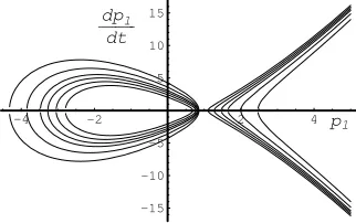
(equation (18)) we plot dp1
dt against p1; this phase portrait is
illustrated for the Euclidean case in Figure 1, the Spherical case in Figure 2 and the Hyperbolic case in Figure 3 with each isocline dependent on the constant I2. The constants
used were M1 =σ= 0.5, H∗= 1, I3= 1 andI2 was set to
different constants1,2,3,4,6,9which correspond to different isoclines in the figures. Each of the three figures vary only by the parameter ε. For each value of I2 there is a bounded
component and an unbounded component, the smallest value ofI2corresponds to the smallest bounded component and the
right most unbounded component:
-2 2 4
-10 -5 5 10
dp1
dt
[image:8.595.340.532.112.237.2]p1
Fig. 1. Phase Portrait- the Euclidean case with increasedI2 the bounded
component becomes larger and the unbounded component shifts to the left
-1 1 2 3 4 5
-10 -5 5 10
dp1
dt
[image:8.595.343.531.289.410.2]p1
Fig. 2. Phase Portrait- the spherical case with increasedI2 the bounded
component becomes larger and the unbounded component shifts to the left
-4 -2 2 4
-15 -10 -5 5 10 15 dp1
dt
p1
Fig. 3. Phase Portrait- the hyperbolic case with increasedI2 the bounded
component becomes larger and the unbounded component shifts to the left
In the physical sense the bounded component is the only one that corresponds to real motions of the vehicle, as the extremals at these values of p1 are real. In all three cases,
provided the roots of the cubic are real the phase portraits are qualitatively unchanged. From the figures it is clear to see that p1 is increasing above the horizontal axis dpdt1 >0 and
decreasing below the horizontal axis dp1
dt <0. It is also clear
to see that any initialization on the bounded component will flow to an equilibrium point i.e equilibrium points lie on the horizontal axis where dp1
dt = 0. It is only the isoclines that
correspond to the unbounded component where dp1
[image:8.595.356.517.467.568.2]do not flow to an equilibrium point. Therefore considering only the possibility of real extremals, ast→ ∞,p1tends to a
constant corresponding to a root of the cubic (18). In addition, as the curvature and torsion are both constant when p1 is
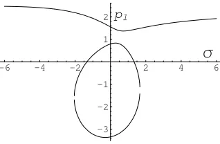
constant, the elastic curves corresponding to real extremals will flow to a helix ast→ ∞. Proceeding, assuming a constant I2, we illustrate the different qualitative behavior of the critical
points depending only on the curvature of the underlying space form. As M1 is the constantσ and can be initialized at any
constant, a plot is given of the roots of the cubic equation f(p1) = 0, withp1 a function ofσ. In each of the following
casesH∗,I
2 andI3 were constant and onlyε was varied. A
plot of the real roots/critical points are given in Figure 4 for ε= 0, Figure 5 forε= 1 and Figure 6 forε=−1:
-6 -4 -2 2 4
2 4 6
p1
[image:9.595.96.256.234.336.2]Σ
Fig. 4. The singularities of the system: Euclidean caseε=0
-6 -4 -2 2 4 6
-4 -2 2 4 6 8
p1
[image:9.595.95.253.381.481.2]Σ
Fig. 5. The singularities of the system: Spherical caseε=1
-6 -4 -2 2 4 6
-3 -2 -1 1 2 p1
Σ
Fig. 6. The singularities of the system: Hyperbolic caseε=-1
The diagrams above give an indication in the differing qualitative nature of the solutions depending on the underlying space form.
C. The geometry of the extremals at the singularity
At the singularity defined at the critical points of the cubic, p1 is constant and will be denoted by c. Then the Casimir
functions (9), (10) and (11) can be written in a reduced form, see [4], where the left hand side of these equations are all constants:
2(H∗−c)−σ
2
c1
=M22+M32
I2−c2−ε(σ2) =p22+p23+ε(M22+M32)
I3−cσ=p2M2+p3M3
(52)
writing the third equation in terms ofp2and squaring gives:
p2 2=
(I2
3−2I3cσ+c2σ2)−2I3p3M3+ 2cσp3M3+p23M32
M2 2
defining new constants α = (I2
3 −2I3cσ+c2σ2) and γ =
I2−c2−ε(σ2)for simplicity, then by substitutingp22into the
second equation in (52), the reduced Hamiltonian and reduced Casimirs can be written as two surfaces in 3 dimensions (p3, M2, M3):
2(H∗−c)−σ
2
c1
=M22+M32
γM22=α+p23M22+ 2cσp3M3−2I3p3M3+p23M32
+εM22(2(H∗−c)−
σ2
c1
)
(53)
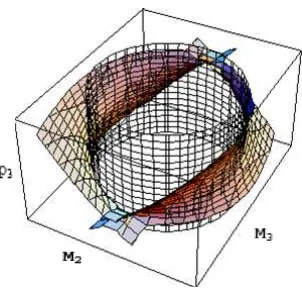
Proceeding more geometrically we analyze the system at the singularities in terms of the intersection of these two invariant surfaces. For the purpose of the following illustration we take ∆ > 0 where ∆ is defined in equation (28) with positive reduced Hamiltonian i.e. the left hand side of the first equation in (52) is assumed positive, in a physical sense this is meaningful as energy is always positive. For each case the 3-dimensional surfaces are drawn graphically in Fig. 7. for ε= 0, Fig. 8. forε= 1 and Fig. 9. forε=−1.
[image:9.595.95.254.524.628.2] [image:9.595.360.513.549.714.2]Fig. 8. The intersection of the energy cylinder and the non-generic quadric forε= 1at the singularity
Fig. 9. The intersection of the energy cylinder and the non-generic quadric forε=−1at the singularity
The surfaces make contact and in each case the intersection is a closed periodic orbit. Fig. 10. shows the points of intersection for ε = 1, this remains qualitatively unchanged in each case ε= 0andε=−1.
-1
0
1 M2
-1 0
1
M3 -0.5
0 0.5
p3
-1
0
1 M2
Fig. 10. Closed periodic orbit; intersection of invariant surfaces
When p1 is constant, M2 and M3 are explicitly solved as
(23), whereris constant andθis linear int. Using the equation from (12)
dM2
dt = M1M3
c1
−M1M3+p3 (54)
and assuming p1 is constant, we differentiate M2 as solved
in (23) and along with the solutions for M1, M2, M3 are
substituted in equation (54) and rearranged to give:
p3=
µ
σ(c1−1
c1 ) + ˙θ
rcos(θ(t)) (55)
where θ˙ is a constant (21) when p1 is constant. Therefore,
in the frame (p3, M2, M3) the explicit solutions describe an
ellipse as shown in Figure 10. To show this let us define a constant λ = ³σ(c1−1
c1 ) + ˙θ ´
r. Clearly, the projection onto the M2, M3 plane is a circle. In addition it is easily shown
that the projection of this ellipse onto the p3, M2 plane is
an ellipse from the explicit solutions and satisfy the implicit elliptic equation.
p2 3
λ2 +
M2 2
r2 = 1 (56)
Thus, the extremal curve is a circle whenλ=r.
D. The explicit solution of the periodic orbit
Recall that assuming only real extremals ast→ ∞,p1tends
to a constant defined by a root of the cubic (18). At these roots the solutions to the Hamiltonian vector fields simplify greatly. Immediately, from (23) whereris constant andθ is linear in t gives:
M2(t) =rsin(θ(t))
M3(t) =rcos(θ(t))
(57)
Then using the equations (12) to obtain the explicit expressions in the same manner as for equation (55) yields:
p2(t) =λsin(θ(t))
p3(t) =λcos(θ(t))
(58)
Therefore, at the critical points wherep1=c is constant, the
explicit solutions (57) and (58) define a closed periodic orbit in the planep1, M1. From equation (21) withp1constant and
assuming the initial value at t= 0 to beθ0= 0then:
θ(t) = Ã
σ c1
−σ+ I3−p1σ 2(H∗−p1)−σ2
c1 !
t
Equating θ to 2nπ where n∈ Z the period T of the closed orbit is:
T = 2nπ/
Ã
σ c1
−σ+ I3−p1σ 2(H∗−p1)−σ2
c1 !
E. The corresponding elastic curves at the singularity (Criti-cal Configurations)
Asκandτ are constant when p1 is constant it is
straight-forward to integrate the equation (29) by taking the matrix exponential map from the Lie algebra to the Lie group (see [18]). An illustration of the different types of elastic curves that correspond to singularities inE3is given. The illustration ofS3andH3are omitted. The plot below shows a bifurcation diagram for the system for a particular set of constants. The critical points of p1 are a function of the constant I2, a plot
[image:10.595.111.240.511.614.2]2 4 6 8 10
-3 -2 -1 1 2 3
I2
[image:11.595.93.257.54.153.2]p1=c
Fig. 11. Bifurcation diagram where the critical points ofp1 are dependent
onI2
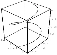
As an illustration of the helical maneuvers of the vehicle we choose I2 = 2 in Figure. 11. such that there are three
real roots; a negative root, a small positive root and a larger positive root. For a fixed length of time, the vehicle traces the following elastic curve γ(t) =g(t)~e1= [x1, x2, x3]T:
-0.2 0
0.2 x1
0 0.2
0.4 x2
0 0.2 0.4 0.6
x3 0
0.2 0.4
[image:11.595.130.220.289.401.2]0 0.2 0.4 0.6
Fig. 12. Helix forp1 = −1.17693and I2 = 2, givingκ = 4.1 and τ= 0.406
When p1 = 0.738226 and I2 = 2, κ = 0.27 and τ =
−7.93. This is not illustrated here as for the same dimensions as Figure.12., the helix appears close to a straight line. Figure. 13. illustrates the helix for the large positive real root
-0.5 0
0.5 1 x1
-1.5 -1
-0.5 0
x2 -1.5
-1 -0.5
0
x3
-0.5 0
0.5 1 x1
-1.5 -1
-0.5
Fig. 13. Helix forp1 = 1.4387andI2 = 2, givingκ =−1.1275 and
τ= 0.279
Although the Serret-Frame gives a geometric interpretation of the elastic curves, it does not give any indication of how the vehicle rotates along these curves. For information about the rotation it is necessary to integrate the general frame (7). However, as the extremals are time dependent the integration procedure is not trivial and is the area of current research.
VI. CONCLUSION
Oriented vehicles travelling at unit speed which are sub-ject to steering controls that change their orientation can be modelled analogously to the elastic problem on Lie groups, where the Lie group describes the configuration space of the vehicle. The configuration spaces considered in this paper are the orthonormal frame bundlesSE(3),SO(4) andSO(1,3). For these systems the extremal curves are solved explicitly in terms of elliptic functions. Under a transformation from the general frame to the Serret-Frenet frame, it is shown that the curvature and torsion of the corresponding elastic curves are also explicitly defined in terms of elliptic functions. In this paper an analysis at a singularity of these systems is given, defined at the roots of a cubic function that appear in the explicit solutions of the extremal curves. At these singularities it is shown that the extremal curves define a periodic orbit and the corresponding elastic curves have constant curvature and torsion. Therefore, the singularities in the extremal curves coincide with steady motions of the vehicle i.e. constant translation and/or constant rotation. Identifying such equilibria is extremely useful in the motion planning of vehicles. Using various stabilization techniques from geometric control such periodic equilibria can be exploited to obtain these steady motions. Although, the focus of this paper is on the motion control of vehicles travelling at unit speed, this paper presents new results applicable to general elastic curves and Kirchhoff’s elastic rod. Future work will include a stability analysis of these singularities and methods to integrate the general frame in order to analyze the rotation of these vehicles as they trace elastic curves.
REFERENCES
[1] Walsh, G., Montgomery, R., Sastry, S., ‘Optimal Path Planning on Matrix Lie Groups’. Proceedings of IEEE Conference on Decision and Control, 1994.
[2] Justh, E. W., Krishnaprasad, P. S., ‘Natural frames and interacting particles in three dimension’. Proceedings of 44th IEEE Conference on Decision and Control and the European Control Conference, 2005. [3] Leonard, N. E., Krishnaprasad, P. S., ‘Motion control of drift-free,
left-invariant systems on Lie groups’. IEEE Transactions on Automatic Control, 40(9):1539-1554, 1995.
[4] Biggs, J. D., Holderbaum, W., ‘The geometry of optimal control problems on some Six dimensional Lie Groups’. Proceedings of 44th IEEE Con-ference on Decision and Control and the European Control ConCon-ference, 2005.
[5] Arroyo, J., Barros, M., Garay, O., ‘Models of relativistic particles with curvature and torsion revisited’. General Relativity and Gravitation, Springer,Volume 36, Number 6, p.1441 - 1451, 2004.
[6] Jurdjevic, V., ‘Geometric Control Theory’. Advanced Studies in Mathe-matics, Cambridge University Press, 52,1997.
[7] Jurdjevic, V., Monroy-Perez, F., ‘Variational Problems on Lie Groups and their Homogeneous Spaces: Elastic Curves, Tops, and constrained Geodesic Problems’ in Nonlinear Geometric Control Theory. World Scientific, 2002.
[8] Bloch, A. M., ‘Nonholonomic Mechanics and Control’. Springer-Verlag, New York,2003.
[9] Crouch, P., Silva Leite, F., ‘The Dynamic interpolation problem: On Riemannian manifolds, Lie groups and Symmetric spaces’. Journal of Dynamical and control systems, Vol.1, No. 2, p177-202, 1995. [10] Bloch, A., Crouch, P., Ratui, T., ‘Sub-Riemannian optimal control
problems’. Fields Institute Communications, vol. 3, pp. 35-48, 1994. [11] Hussein, I. I., Bloch, A. M., ‘Optimal control of under-actuated systems
[image:11.595.127.223.527.621.2][12] Sussmann, H. J., ‘An introduction to the coordinate-free Maximum Principle’. In Geometry of Feedback and Optimal Control,B. Jakubczyk and W. Respondek Eds., Marcel Dekker, New York, pp. 463-557, 1997. [13] Jurdjevic, V., ‘Integrable Hamiltonian Systems on Complex Lie Groups’. Memoirs of the American Mathematical Society, Vol. 178, No. 838, 2005. [14] Ott, E., ‘Chaos in Dynamical Systems’. Cambridge University Press,
1993.
[15] Goyal, S., Perkins, N. C., Lee, C. L. ‘Nonlinear dynamics and loop formation in Kirchhoff rods with implications to the mechanics of DNA and cables’. Journal of Computational Physics, Vol. 209, Issue 1, pp. 371-389, 2005.
[16] Audin, M., ‘Spinning Tops: A course on Integrable Systems’. Advanced Studies in Mathematics, Cambridge University Press, 1996.
[17] Lawden, D., ‘Elliptic functions and applications’. Springer-Verlag, New York, 1989.
[18] Hall, B. C., ‘Lie Groups, Lie Algebras, and Representations: An Elementary Introduction’. Springer-Verlag, New York, 2003.
James Biggs received the B.Sc. degree in Math-ematics with Economics from the University of Sussex, Brighton, UK in 1998 and the M.Sc. degree in Nonlinear Dynamics and Chaos from University College London, London, U.K. in 1999. Since then he has worked in Operational Research for the Defence Evaluation and Research Agency, U.K. He is currently a final year PhD student at the School of Systems Engineering, University of Reading, Read-ing, U.K. and his current research interests include geometric control theory and its applications.
William Holderbaum received the M.Sc. degree in automatic control from the University of Reims, Reims, France 1993 and the PhD degree from the University of Lille, Lille, France 1999. He was a research assistant at the University of Glasgow, Glas-gow, UK (1999-2001). He is currently a Lecturer in the School of Systems Engineering, University of Reading, Reading, U.K. His research interests are in control theory and its applications. These are mainly focused on boolean input systems (i.e., power converters), rehabilitation engineering (robust control design for unsupported paraplegic standing), and geometric control theory.