optimal control problems for control and
mechanical control systems
Mar´ıa Barbero Li˜n´an
Supervisor: Dr. Miguel C. Mu˜noz Lecanda
A thesis submitted for the Degree of Doctor of Philosophy in Applied Mathematics Department of Applied Mathematics IV
Technical University of Catalonia October 2008
For the last forty years, differential geometry has provided a means of understanding optimal control theory. Usually the best strategy to solve a difficult problem is to transform it into a different problem that can be dealt with more easily. Pontryagin’s Maximum Principle provides the optimal control problem with a Hamiltonian structure. The solutions to the Hamiltonian problem, satisfying particular conditions, are candidates to be solutions to the optimal control problem. These candidates are called extremals. Thus, Pontryagin’s Maximum Principle lifts the original problem to the cotangent bundle.
In this thesis, we develop a complete geometric proof of Pontryagin’s Maximum Principle. We investigate carefully the crucial points in the proof such as the perturbations of the controls, the linear approximation of the reachable set and the separation condition.
Among all the solutions to an optimal control problem, there exist the abnormal curves. These do not depend on the cost function we want to minimize, but only on the geometry of the control system. Some work has been done in the study of abnormality, although only for control–linear and control–affine systems with mainly control–quadratic cost functions. Here we present a novel geometric method to characterize all the different kinds of extremals—not only the abnormal ones—in general optimal control problems. This method consists of adapting conveniently the presymplectic constraint algorithm. Our interest in the abnormal curves is with the strict abnormal minimizers, whose existence was proved in the 90’s in the problem of the shortest paths in subRiemannian geometry. These last minimizers can be characterized by the geometric algorithm presented in this thesis.
As an application of the above–mentioned method, we characterize the extremals for the free optimal control problems that include, in particular, the time–optimal control problem. Moreover, an example of an strict abnormal extremal for a control–affine system is found using the geometric method.
Furthermore, we focus on the description of abnormality for optimal control problems for mechanical control systems, because no results about the existence of strict abnormal minimiz-ers are known for these problems. Results about the abnormal extremals are given when the cost function is control–quadratic or the time must be minimized. In this dissertation, the abnormal-ity is characterized in particular cases through geometric constructions such as vector–valued quadratic forms that appear as a result of applying the previous geometric procedure.
In this thesis, the optimal control problems for mechanical control systems are also tack-led taking advantage of the equivalence between nonholonomic control systems and kinematic control systems. As a result of this approach, it is found an equivalence between time–optimal control problems for both control systems. The results allow us to give an example of a local strict abnormal minimizer in a time–optimal control problem for a mechanical control system.
Finally, setting aside the abnormality, the non–autonomous optimal control problem is de-scribed geometrically using the Skinner–Rusk unified formalism. This approach is valid for
iv Abstract
implicit control systems that arise, for instance, in optimal control problems for the controlled Lagrangian systems and for descriptor systems. Both systems are common in engineering prob-lems.
Dr. Miguel Carlos Mu˜noz Lecanda, chair in Applied Mathematics,
CERTIFIES
that this report with the title
A geometric study of abnormality in optimal control problems for control and mechanical control systems
has been composed and originated in the Department of Applied Mathematics IV at the Tech-nical University of Catalonia under his supervision, by Mar´ıa Barbero Li˜n´an and gives his permission so as to be qualified as a Ph.D. dissertation.
T
his dissertation would not have been possible without the support and the guidance provided by my supervisor, Dr. Miguel C. Mu˜noz Lecanda at every single moment. These last fours years working under his supervision have made me grow as a researcher and as a person. I am also grateful to Professor Andrew D. Lewis as a non–official supervisor for encouraging me to work on a deep understanding of optimal control theory during his sabbatical stay in Barcelona. I would also like to thank him for accepting me as a visiting student in his department and for continuously showing interest in my work. He is always willing to share his eye–opening new ideas with others.I would like to thank the anonymous referees of journals and conferences because they helped to improve my work with their comments.
I am grateful to have become part of the research group DGDSA in the Department of Applied Mathematics IV at the Technical University of Catalonia. Narciso, Arturo and Xavier gave me a warm welcome from the first day and always show their interest in my work. I would like to thank especially Narciso for sharing his teaching duties with me and taking care of my bamboo.
I would like to thank the research network Geometry, Mechanics and Control that has given me the opportunity to attend international conferences and to interact with expert researchers like David Mart´ın de Diego (who even invited me to go to Madrid to make me go into the world of Lie algebroids), Eduardo Mart´ınez, and Juan Carlos Marrero who were always willing to discuss my research and help me with different viewpoints. I do not forget the young people in this research network who always create a great environment for everything, also thanks to them. A special thank goes to Edith who always succeeds in coordinating all the issues in an unbeatable way, it is just astonishing.
The financial support ofMinisterio de Educaci´on y Ciencia—Project MTM2005-04947, the Network Project MTM2006-27467-E/ and an FPU grant— and ofGeneralitat de Catalunya with an FI grant have been essential to be able to devote my energy to research.
I would like to thank the staff and colleagues in the Department of Applied Mathematics IV in Barcelona and in the Department of Mathematics and Statistics at Queen’s University in Kingston (Ontario, Canada) for their continuous help. In Kingston I had the pleasure to join Professor Lewis’ group where I found PhD students with common grounds, above all, Bahman and Cesar. I have always enjoyed the discussions and seminars we had together.
I am grateful to my friends and to my family in Barcelona because they have been there to listen to me, to cheer me up and to give me different opinions. All of them have made this period of my life enjoyable, even when I was forced to take a few months off. I would like to express my gratitude to all of them because they were there taking care of me when I most
viii Acknowledgements
needed. Special thanks to Ciara, Anna, Bernat, Ver´onicas, Mar´ıa, ´Oscar, Oriol, Marina, Puri, Mary C´armenes, Carmen and Elena.
Finally, to my parents because I know it has not been easy to accompany me through this process. Not all the news I had for you were the ones you have liked to listen. In spite of that, you always give me your love and unconditional support. To my brother, you are always in the lead and so I can benefit from your experience, professionally and personally. To James, you have given a different meaning to my life since we met. To be able to type the first draft of this thesis next to you made it pleasant.
Contents
Abstract . . . iii
Certification . . . v
Acknowledgements . . . vii
Contents . . . ix
List of Figures . . . xiv
Acronyms . . . xv
List of Symbols . . . xvi
1 Introduction 1 1.1 Historical remarks . . . 1
1.2 State–of–the–art . . . 2
1.3 Contributions and scheme of the thesis . . . 5
2 Background and notation 9 2.1 Manifolds and tensor fields . . . 9
2.2 Time–dependent vector fields . . . 13
2.2.1 Vector fields along a projection . . . 14
2.2.2 Time–dependent variational equations . . . 15
2.2.2.1 Complete lift . . . 15
2.2.2.2 Cotangent lift . . . 18
2.2.2.3 A property for the complete and cotangent lift . . . 19
2.3 Symplectic geometry . . . 19
2.3.1 Symplectic manifolds . . . 20
2.3.2 Presymplectic constraint algorithm . . . 20
2.4 Ehresmann connections . . . 22
2.4.1 Notion of connection . . . 22
2.4.2 Connection associated with an almost product structure on a fiber bundle 24 2.4.3 Splitting ofT∗Eaccording to an Ehresmann connection . . . 26
2.4.4 Linear Ehresmann connection . . . 26
2.4.5 Dual of a linear Ehresmann connection . . . 28
2.4.6 Induced Ehresmann connection onτM:TM→Massociated with a second–order differential equation . . . 29
2.5 Skinner–Rusk unified formalism for non–autonomous systems . . . 31
2.6 Particular background in jet bundles . . . 34
2.6.1 Jet bundles of order 1 and 2 . . . 34
2.6.2 Tulczyjew’s operators . . . 35
2.6.3 Implicit Euler–Lagrange equations . . . 36
3 Background in control theory 39 3.1 Control systems . . . 39
3.2 Accessibility and controllability . . . 40
4 Geometric Pontryagin’s Maximum Principle 45
4.1 Pontryagin’s Maximum Principle for fixed time and fixed endpoints . . . 46
4.1.1 Statement of optimal control problem and notation . . . 46
4.1.2 The extended problem . . . 47
4.1.3 Perturbation and associated cones . . . 48
4.1.3.1 Elementary perturbation vectors: class I . . . 49
4.1.3.2 Perturbation vectors of class II . . . 52
4.1.3.3 Perturbation cones . . . 55
4.1.4 Pontryagin’s Maximum Principle in the symplectic formalism for the optimal control problem . . . 59
4.2 Proof of Pontryagin’s Maximum Principle for fixed time and fixed endpoints . . 64
4.3 Pontryagin’s Maximum Principle for nonfixed time and nonfixed endpoints . . 72
4.3.1 Statement of the optimal control problem with nonfixed time and non-fixed endpoints . . . 72
4.3.2 Perturbation of the time and the endpoints . . . 73
4.3.2.1 Time perturbation vectors and associated cones . . . 73
4.3.2.2 Perturbing the endpoint conditions . . . 77
4.3.3 Pontryagin’s Maximum Principle in the symplectic formalism for non-fixed time and nonnon-fixed endpoints . . . 79
4.4 Proof of PMP for nonfixed time and nonfixed endpoints . . . 81
4.5 Abnormality, controllability and optimality . . . 84
4.5.1 Generalization of the notion of linear controllable . . . 84
4.5.2 The tangent perturbation cone as an approximation of the reachable set 86 4.6 Examples . . . 89
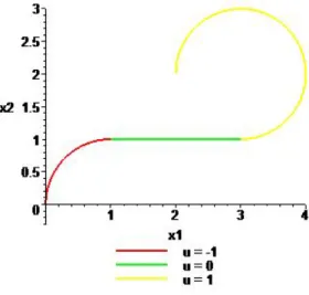
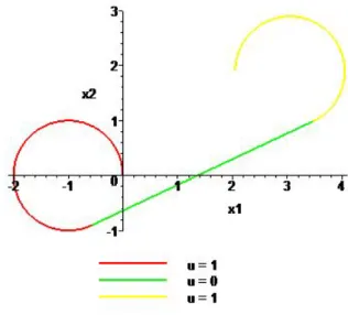
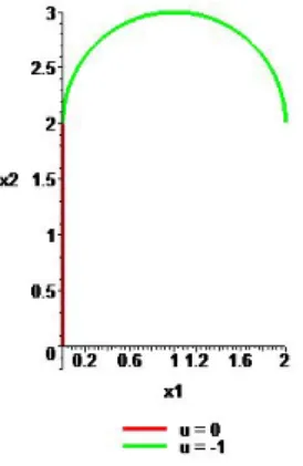
4.6.1 Dubins car . . . 89
4.6.2 A strict abnormal optimal solution . . . 97
5 Constraint algorithm for the extremals 103 5.1 Presymplectic Pontryagin’s Maximum Principle . . . 103
5.2 Characterization of extremals . . . 105
5.2.1 Characterization of abnormality . . . 107
5.2.2 Characterization of normality . . . 107
5.2.3 Characterization of strict abnormality . . . 109
5.3 Free optimal control problem . . . 110
5.4 Examples revisited . . . 111
5.4.1 Geodesics in Riemannian geometry . . . 111
5.4.2 SubRiemannian geometry . . . 112
5.4.3 Control–affine systems . . . 114
5.5 A strict abnormal extremal in a control–affine system . . . 115
6 Pontryagin’s Maximum Principle for mechanical systems 119 6.1 Affine connection control systems . . . 120
6.2 Accessibility and controllability for mechanical systems . . . 121
6.3 Optimal control problem for affine connection control systems . . . 124
6.4 Intrinsic mechanical Pontryagin’s Maximum Principle . . . 125
6.4.1 Useful splittings . . . 126
xii Contents
6.4.1.2 Splitting ofT∗TQaccording to the linear connection onτQ. 127
6.4.1.3 Dual of a linear connection onτQ:TQ→Qassociated with
an affine connection onQ . . . 127
6.4.1.4 Linear connection onτTQ:TTQ→TQassociated with an affine connection onQ . . . 128
6.4.1.5 Dual of a linear connection onτTQ:TTQ→TQ associ-ated with an affine connection onQ. . . 129
6.4.2 Intrinsic Pontryagin’s Maximum Principle for affine connection control systems . . . 130
6.5 Weak mechanical Pontryagin’s Maximum Principle . . . 132
6.6 Constraint algorithm for extremals in OCP for ACCS . . . 133
6.6.1 Characterization of abnormality . . . 134
6.6.2 Characterization of normality . . . 137
6.7 Applications to optimal control problems . . . 137
6.7.1 Some control–quadratic cost functions . . . 137
6.7.2 Time–optimal control problem . . . 139
6.8 Study of abnormality for particular cases . . . 140
6.8.1 Fully actuated . . . 141
6.8.2 One control vector field in two dimension . . . 141
6.8.3 Underactuated by one input . . . 143
7 Strict abnormal extremals in nonholonomic and kinematic control systems 147 7.1 Optimal control problem: nonholonomic versus kinematic . . . 148
7.1.1 Nonholonomic mechanical systems with control . . . 148
7.1.2 Associated optimal control problems . . . 149
7.2 Hamiltonian problems for nonholonomic versus kinematic . . . 153
7.2.1 Nonholonomic Pontryagin’s Hamiltonian and extremals . . . 154
7.2.2 Kinematic Pontryagin’s Hamiltonian and extremals . . . 156
7.2.3 Connection between nonholonomic and kinematic momenta . . . 157
7.2.4 Example . . . 158
8 Skinner–Rusk unified formalism for optimal control systems and applications 163 8.1 Non–autonomous optimal control problems . . . 164
8.1.1 Unified geometric framework for optimal control theory . . . 165
8.1.2 Optimal control equations . . . 168
8.2 Implicit optimal control problems . . . 170
8.2.1 Unified geometric framework for implicit optimal control problems . . 171
8.2.2 Optimal control equations . . . 173
8.3 Applications and examples . . . 175
8.3.1 Optimal control for the controlled Lagrangian systems . . . 175
8.3.2 Optimal control problems for descriptor systems . . . 179
9 Conclusion and future work 183 9.1 Summary of the contributions . . . 183
9.2 Future work . . . 184
9.2.1 Search for strict abnormal minimizers . . . 184
9.2.3 Geometric high–order Maximum Principle . . . 185 9.2.4 The algebra of accessibility without zero velocity . . . 186
A Background in analysis 189
A.1 Results on real functions . . . 189 A.2 Lebesgue points for a real function . . . 190 A.3 One corollary of Brouwer Fixed–Point Theorem . . . 192
B Convex sets, cones and hyperplanes 193
B.1 Convex sets and cones . . . 193 B.2 Distinguished hyperplanes . . . 195
C Vector–valued quadratic forms 199
C.1 Definition and properties . . . 199 C.2 A particular vector–valued quadratic form . . . 200
List of Figures
2.1 Idea of the linear approximation of integral curves of a vector field. . . 17
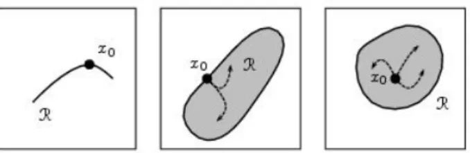
3.1 No accessible, accessible and controllable . . . 42
4.1 Elementary perturbation ofuspecified by the dataπ1and the integral curve on M ofX{u[π1s]}. . . 49
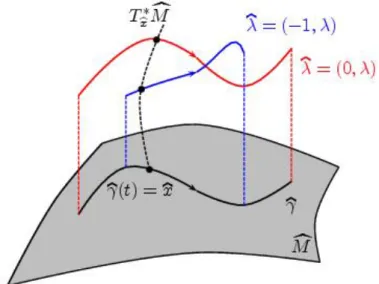
4.2 An optimal curve with two different lifts to T∗Mcso that it is abnormal and normal at the same time. . . 63
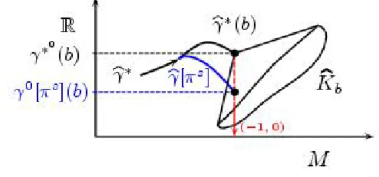
4.3 Situation if(−1,0) b γ∗(b)is interior toKbb. . . 65
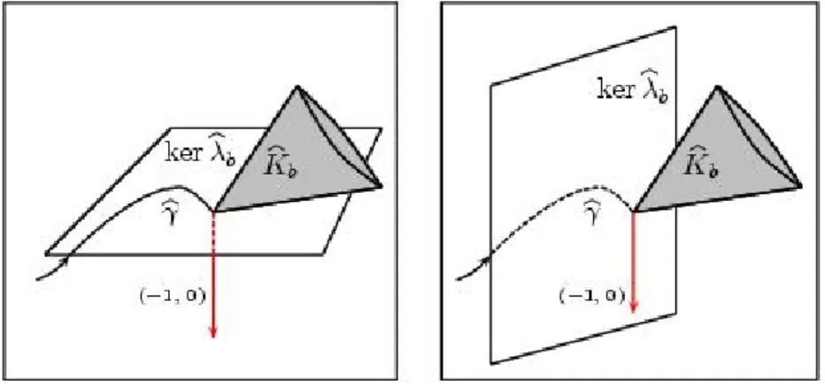
4.4 Separation condition for an extremal being normal and abnormal, respectively. . 72
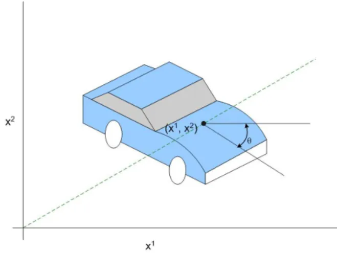
4.5 Dubins car. . . 90
4.6 The value of the functional for this trajectory is2 + 2πseconds. . . 94
4.7 The value of the functional for this trajectory is 13.89 seconds. . . 95
4.8 The value of the functional for this trajectory is2 +πseconds. . . 97
4.9 Reachable set from(0,0)up to π given by curves that have been associated with a momenta satisfying Hamilton’s equations forp0=−1. . . 98
4.10 Reachable set from(0,0)up to timeπgiven by curves that have been associated with a momenta satisfying Hamilton’s equations forp0= 0. . . 99
4.11 Separation condition att= 1for the normal momenta. . . 100
4.12 Separation condition att= 1for the abnormal momenta. . . 101
4.13 The separation condition att = 3for the momenta obtained from Hamilton’s equations forp0 =−1is not satisfied. . . 101
4.14 Separation condition att= 3for the abnormal momenta. . . 102
4.15 Reachable set from (0,0,0)up to time π of the extended control system of (4.6.23). . . 102
ACCS Affine connection control systems
FHP Free Hamiltonian problem
FOCP Free optimal control problem
\
FOCP Extended free optimal control problem FPMP Free Pontryagin’s Maximum Principle
HP Hamiltonian problem
OCP Optimal control problem
[
OCP Extended optimal control problem PMP Pontryagin’s Maximum Principle STLC Small–time locally controllable
List of Symbols
a.e. almost everywhere
a.c. absolutely continuous
M m–dimensional manifold
Q n–dimensional manifold
U Control set inRk
T M Tangent bundle ofM
T∗M Cotangent bundle ofM
τM Canonical tangent projection
πM Canonical cotangent projection
C∞(M) Set of smooth real–valued functions onM X(M) Set of vector fields onM
Ω1(M) Set of1–forms onM
T(M) Set of all the tensor fields onM
f∗ Pullback of theC∞–functionf
f∗ Pushforward of a diffeomorphismf:M →M
d Exterior derivative
iX, i(X) Inner or interior product of a vector fieldXonM
I Compact interval inR
φXx0 Integral curve of the vector fieldX with initial conditionx0 at time
zero
Γ(π) Set of sections of the fiber or the vector bundleπ
V(π) Vertical subbundle ofπ
XV(M, π) Set of vertical vector fields onMwith respect toπ X(π) Set of vector fields along a projectionπ
D0
x=D⊥x = annDx Annihilator of the distributionDatx
∇ Affine connection on a manifold
∇XY Covariant derivative ofY with respect toX
ΦX Time–dependent flow or evolution operator of the time–dependent vec-tor fieldXonM
XT Complete or tangent lift of the vector fieldX
κM Canonical involution ofT T M
X{u} Time–dependent vector field onMsuch thatX{u}(t, x) =X(x, u(t)).
XT∗ Cotangent lift of the vector fieldX
LX Lie derivative operator with respect to the vector fieldX
∆ Liouville vector field on a vector bundleπ:E →B
JM Vertical endomorphism
J1π The jet bundle of sections ofπ
W Extended jet–momentum bundle
Wr Restricted jet–momentum bundle
ˆ
C Coupling1–form inW
fs, Ys Control vector fields on a manifold
(γ, u) A curve on a manifoldM×U orQ×U
F Cost function
S[γ, u] Functional to be minimized
(M, U, X,F, I, xa, xb) Optimal control problem
c
M Extended manifold,R×M
b
γ Curve on the extended manifoldMc
b
X Vector fieldXextended to the manifoldMc
(γ∗, u∗) Solution to an optimal control problem
(M , U,c X, I, xb a, xb) Extended optimal control problem π1={t1, l1, u1} Perturbation data for the control
u[πs1] Perturbation ofuspecified by the dataπ1
v[π1] Elementary perturbation vector associated to the perturbation dataπ1
V[π1] Integral curve of(XT){u} with initial conditionv[π1]att1
Kt Tangent perturbation cone at timet
B(p, r) Open ball in the Euclidean space at centerpwith radiusr B(p, r) Closed ball in the Euclidean space at centerpwith radiusr
H (Pontryagin’s) Hamiltonian function
b
λ Extended momenta onT∗Mcgiven by Pontryagin’s Maximum
Princi-ple
xviii List of Symbols
Kt± Time perturbation cone at timet
Ni[0] Constraint submanifold at stepifor abnormality
Ni[−1] Constraint submanifold at stepifor normality
Y ={Y1, . . . , Yk} Family of control or input vector fields
Σ = (Q,∇,Y, U) Affine connection control system
ΣF(xa, xb) Optimal control problem for an affine connection control system with
endpoint conditionsxa, xb inQ
Υ A curve on the tangent bundleT Q
Z Geodesic spray associated with a connection∇ h·:·i Symmetric product of two vector fields
Λ Momenta onT∗T Qgiven by the mechanical Pontryagin’s Maximum Principle
Bx Vector–valued quadratic form atx∈Q
(λB)x Real quadratic form inherited fromBxforλ∈annYx
ΣD= (Q, g, F,D) Nonholonomic control system
Σm= (ΣD,F) Nonholonomic optimal control problem for the systemΣD with cost
functionF
Σk= (Σm,G) Kinematic optimal control problem for the kinematic control system
associated toΣmwith cost functionG
Hm Pontryagin’s Hamiltonian function for the problemΣm
Hk Pontryagin’s Hamiltonian function for the problemΣk
b
a Extended momenta associated with the problemΣkor extended
kine-matic momenta
b
vm Extended perturbation vectors associated withΣm
b
vk Extended perturbation vectors associated withΣk
WX Extended control–jet–momentum bundle
WX
r Restricted control–jet–momentum bundle
WMC Extended control–jet–momentum bundle for implicit optimal control
problems
WMC
r Restricted control–jet–momentum bundle for implicit optimal control
Introduction
Optimal control theory is a young research area that appears in a wide variety of fields such as medicine, economics, traffic flow, engineering, astronomy. However, applications and un-derstanding do not always come together. In order to gain insight, differential geometry has been used in control theory, giving rise to geometric control theory in the 70’s [Agrachev 2002a, Agrachev and Sachkov 2004, Bloch 2003, Bonnard and Caillau 2006, Bonnard and Chyba 2003, Boscain and Piccoli 2004, Bressan and Piccoli 2007, Bullo and Lewis 2005a;b, Echeverr´ıa-Enr´ıquez et al. 2003, Jurdjevic 1997, Langerock 2003a, Lewis 2006, Nijmeijer and van der Schaft 1990, Sussmann 1978; 1998; 1999; 2000, Sussmann and Jurdjevic 1972, Trout-man 1996].1.1
Historical remarks
If we look back in time, we will realise that optimal control problems have existed for a long time as claimed by Sussmann and Willems [1997]. There, the brachystochrone problem sug-gested by J. Bernoulli in the June 1696 issue ofActa Eruditorumis considered as the starting point of optimal control theory. The challenge posed to mathematicians by J. Bernoulli is the following:
If, in a vertical plane, two pointsA and B are given, then it is required to specify the orbitAM Bof the movable pointM, along which it, starting from
A, and under the influence of its own weight, arrives at B in the shortest possible time. So that those who are keen of such matters will be tempted to solve this problem, is it good to know that it is not, as it may seem, purely speculative and without practical use. Rather it even appears, and this may be hard to believe, that it is very useful also for other branches of science than mechanics. In order to avoid a hasty conclusion, it should be remarked that the straight line is certainly the line of shortest distance betweenA and B, but it is not the one which is traveled in the shortest time. However, the curve
AM B—which I shall divulge if by the end of this year nobody else has found it—is very well known among geometers.
Thus, control theory studies the properties of a dynamical system with some degrees of freedom given by the controls; e.g., in the previous problem those are associated with the point
M. When we want to find the trajectory of a dynamical system that minimizes a functional such as energy, time or distance, we are confronting a problem in optimal control. In general, to find a solution of these kinds of problems is not straightforward. A valuable tactic to deal with
2 1.2. State–of–the–art
optimal control problems is to restrict the candidate solutions through necessary conditions of optimality such as those given by Pontryagin’s Maximum Principle [Pontryagin et al. 1962].
In some sense, optimal control theory is regarded as a generalization of the calculus of vari-ations [Bullo and Lewis 2005b, Lewis 2006, Sussmann and Willems 1997]. A main difference between these two theories is that in the former the controls can take values in a closed control set and inequality constraints are accepted, whereas in the latter the control set is always open. Pontryagin’s Maximum Principle was introduced to the mathematical community in the International Congress of Mathematicians held in 1958 in Edinburgh, Scotland, by a group of Russian researchers working in Steklov Mathematical Institute [Pontryagin et al. 1962]. The Russian school focused on this research under a request by the military service. The Maximum Principle is considered one of the outstanding points in optimal control theory.
1.2
State–of–the–art
The classical approach to optimal control problems was from the point of view of the differ-ential equations [Athans and Falb 1966, Lee and Markus 1967, Pontryagin et al. 1962] and of the functional analysis [Giaquinta and Hildebrandt 1996a;b, Zeidler 1985], but later the ap-proach was from the differential geometry [Agrachev and Sachkov 2004, Bressan and Piccoli 2007, Jurdjevic 1997, Sussmann 1998]. However, the Maximum Principle admits other points of view such as stochastic control systems [Bensoussan 1984, Haussmann 1986] and discrete control systems [Chyba et al. 2008, Guibout and Bloch 2004, Hwang and Fan 1967]. Lately, the Skinner-Rusk formulation [Skinner and Rusk 1983] has been applied to study optimal control problem for non–autonomous control systems. As a result, the necessary conditions of Pon-tryagin’s Maximum Principle have been obtained, as long as the differentiability with respect to controls is assumed [Barbero-Li˜n´an et al. 2007].
A Hamiltonian formalism to optimal control problems is provided by the necessary condi-tions stated in Pontryagin’s Maximum Principle. The solucondi-tions to the problem are in a manifold, but the Maximum Principle relates solutions to a lift to the cotangent bundle of that manifold. Thus, in order to find candidate optimal solutions, not only the controls but also the momenta must be chosen appropriately so that the necessary conditions in the Maximum Principle are fulfilled. These conditions are, in fact, first–order necessary conditions and they are not always enough to determine all the degrees of freedom in the problem. That is why sometimes it is necessary to use the high–order Maximum Principle [Bianchini 1998, Kawski 2003, Knobloch 1981, Krener 1977]. But, even when we succeed in finding the controls and the momenta in such a way that Hamilton’s equations can be integrated to obtain a trajectory on the manifold, the controls and the momenta are not necessarily unique. In other words, different controls and different momenta can give the same trajectory on the manifold, although the necessary conditions in the Maximum Principle will be satisfied in different ways. The momenta and the control determine the kinds of trajectories, which can be abnormal, normal, strict abnormal, strict normal and singular. We point out that these different kinds of extremals do not provide a partition of the set of trajectories in the manifold, because it may happen that a same trajectory admits more than one momenta so that the trajectory is in two different categories.
be optimal [Hamenst¨adt 1990, Strichartz 1986]. The idea was that abnormal extremals were isolated curves and thus it was impossible to consider any variation of these curves. However, Montgomery [1994] proved that there exist abnormal minimizers by giving an example in sub-Riemannian geometry. Then Liu and Sussmann [1995] made an effort to characterize strictly abnormal minimizers in a general way for the length-minimizing problem in subRiemannian geometry if there are only two controls. They succeeded in giving a set with abnormal extremals that contains strict abnormal curves that are locally optimal for the considered control–linear system [Liu and Sussmann 1994a;b; 1995, Sussmann 1996]. Let us give a short review of some work that has been done concerning abnormal extremals.
Agrachev and Sarychev [1995b; 1996] study second–order necessary conditions for op-timality since the first–order necessary conditions give little information about abnormal ex-tremals. They state necessary and sufficient conditions for local optimality and rigidity (i.e., isolation) of abnormal extremals using the derivatives of the endpoint mapping, related to the reachable set. They also use the theory of the Morse index.
Agrachev and Sarychev [1995a; 1996] consider subRiemannian geometry for a distribution of rank2. They arrive at the same definition of regular abnormal extremals given by Liu and Sussmann [1995], but they also focus on control–affine systems. They also prove that when the distribution is bracket–generating and the controls are constrained there exist local rigid abnormal minimizers, something that does not happen for unconstrained controls.
Agrachev and Zelenko [2007] characterize the affine line subbundle that gives the abnormal extremals for control–affine systems with one or two input vector fields. For two input vector fields, they concentrate on the study of manifolds of dimension4and5.
Bonnard and Tr´elat [2001] characterize the abnormal directions looking at the subRiema-nnian sphere. In order to do this, they consider mainly the case of Martinet distributions.
Boscain and Piccoli [2002] study the time–optimal control problem for a control–affine system with one input vector field. It turns out that the abnormal extremals are concatenations of determined arcs coming from switching the control. They establish a classification of all the possibilities.
Langerock [2001; 2003a;b;c] characterizes the abnormal extremals geometrically by con-structing a suitable connection.
What makes abnormal extremals more special is that the abnormality does not depend on the cost function. Hence, the abnormal extremals can be determined exclusively using the ge-ometry of the control system. Thus abnormality and controllability must be closely related. In fact, in order to have abnormal minimizers, the system cannot be controllable. Moreover, the set of the trajectories given by the control system determines the reachable set, independently of the cost function. That is why it is thought that the study of the reachability and/or the control-lability [Jurdjevic 1997, Nijmeijer and van der Schaft 1990, Sussmann 1978; 1987] could help to characterize abnormal extremals through the geometry of the reachable set [Bullo and Lewis 2005b, Langerock 2003a]. In control theory, controllability is still one of the properties under active research [Agrachev 1999, Aguilar and Lewis 2008, Basto-Gonc¸alves 1998, Bullo and Lewis 2005c, Cort´es and Mart´ınez 2003, Tyner 2007] and the same happens with abnormality in optimal control theory as already shown.
4 1.2. State–of–the–art
In contrast to the previous paragraph, the cost function is essential to prove that abnormal extremals are strict abnormal minimizers. That is why the existence or non–existence of ab-normal minimizers is only known for specific control problems, mainly time–optimal control problems and optimal control problems with control–quadratic cost functions for control–linear and control–affine systems [Agrachev and Sarychev 1995a; 1999, Agrachev and Zelenko 2007, Bonnard and Chyba 2003, Chitour et al. 2006; 2008, Tr´elat 2001, Zelenko 1999].
In general, the necessary conditions given by the Maximum Principle are useful for de-termining the control that will give us a possible optimal trajectory, except for abnormal and singular extremals [Kupka 1987, Pelletier 1999, Zelenko 1999]. In such cases, it is necessary to consider high–order necessary conditions that will help us to determine the control, as studied by Krener [1977].
When a problem is difficult to deal with, we restrict to particular cases in order to figure out a first idea of possible solutions. That is why we restrict Pontryagin’s Maximum Principle to optimal control problems for mechanical systems described by affine connections [Bullo and Lewis 2005b]. Singular extremals have already been studied in [Chyba and Haberkorn 2005, Chyba et al. 2003]. In fact, the singular extremals are also abnormal for time–optimal problems. The main aim of this dissertation is to give a detailed geometric study of how to characterize abnormal extremals in nonlinear control theory and also for particular cases such as mechanical control systems and control–affine systems. We believe that a better geometric understanding of abnormality will give insights into strict abnormality because every strict abnormal optimal curve is also an abnormal optimal curve.
In order to achieve our aim, we have gone through the entire proof of Pontryagin’s Max-imum Principle translating it into a geometric framework, but preserving the outline of the original proof. All details have been carefully proved, making us to go into the details of con-cepts such as time–dependent variational equations and their properties, perturbation vectors and the separation conditions given by hyperplanes. Afterwards, we focus on some geometric approaches to the abnormality, establishing connections with the controllability.
Then we propose a method to characterize all the different kinds of extremals for any op-timal control problem for any control system. In order to do that, the presymplectic theory is used to adapt the so–called presymplectic constraint algorithm by Gotay and Nester [1979], Gotay et al. [1978].
The next step is the study of the abnormality for affine connection control systems that model mechanical systems. After applying the adapted presymplectic constraint algorithm, we consider particular optimal control problems in order to give more information about the different extremals. Then, we focus on some examples with small dimension where geometric elements, as for instance, the symmetric product and the vector–valued quadratic forms, arise in the reasoning about abnormality. Some ideas between these elements and the abnormality are given.
We consider another approach to study the abnormality for the mechanical case that consists of taking advantage of the results known in subRiemannian geometry. The control system in the problem of finding the shortest paths in subRiemannian geometry is a kinematic control system. Thus, we look into the nonholonomic control systems and their equivalence with the kinematic
control system [Bloch 2003, Bullo and Lewis 2005a;c, Mu˜noz-Lecanda and Y´aniz-Fern´andez 2008] in order to find some connection between the optimal control problems associated with both control systems.
Finally, we put aside our interest in abnormality, and we focus on the Skinner–Rusk for-malism to give a unified approach to the non–autonomous optimal control problems.
1.3
Contributions and scheme of the thesis
Here let us point out the contributions in the area of differential geometry and optimal control theory provided by this dissertation. We also give a brief description of the contents of every chapter.
Chapter 2
This chapter is a review of the main elements of differential geometry used in this disser-tation. A special importance is given to the study of the time–dependent variational equations, the different definitions of a connection on a fiber bundle and the Skinner–Rusk formalism for non–autonomous systems.
In spite of being a review, the study of the time–dependent variational equations given in §2.2.2 gives a clear picture of the flows of the complete lift and of the cotangent lift of a time–dependent vector field via Propositions 2.2.3, 2.2.4, 2.2.6 and Corollary 2.2.5. These results although known, to our knowledge, have not appeared in the literature.
Chapter 3
In this chapter we give the background in control theory necessary for the understanding of the subsequent chapters. We focus mainly on the notion of linear controllable and on the sufficient conditions for controllability.
Chapter 4
Our main contribution is the complete geometric version of the proof of Pontryagin’s Max-imum Principle in§4.2 and§4.4 in a symplectic framework, with all the details about the differ-ent perturbation vectors in§4.1.3 and§4.3.2. The complete proof we give of Proposition 4.1.12, although known, to our knowledge, there is not a self–contained proof of it in the literature.
In§4.5, we give a necessary condition for abnormality, valid for any optimal control prob-lem and related with controllability, Proposition 4.5.2. The proof of Pontryagin’s Maximum Principle suggests that all the perturbation vectors generate a linear approximation of the reach-able set in some sense. That sense will become clear in§4.5.2 and in Proposition 4.5.3, which proves a result often assumed as true in the literature.
Finally, we are able to give a picture of the separation condition for a particular example in
§4.6.2 to show the differences when there exist momenta associated with the trajectory such that it is both abnormal and normal. We will see that the separation condition is another key point in the proof of Pontryagin’s Maximum Principle and must be well–understood geometrically to understand abnormality.
6 1.3. Contributions and scheme of the thesis
Chapter 5
The Maximum Principle is treated from the presymplectic viewpoint. We have two different versions of Hamilton’s equations where the presymplectic constraint algorithm in the sense of Gotay and Nester [1979], Gotay et al. [1978] can be applied.
Apart from the new results in§5.2.1 and§5.2.2, Proposition 5.2.9 summarizes how to use the algorithm to characterize the different kinds of extremals when the domain of definition of the curves is known. If the domain is not given, the adaptation of the presymplectic constraint algorithm is described in§5.3.
To highlight the generality of the geometric process described, the usual examples in the literature are revisited in§5.4: geodesics in Riemannian and in subRiemannian geometry, and optimal control problems for control–affine systems.
In§5.5, we give for first time to our knowledge, a strict abnormal extremal for an optimal control problem for a mechanical control system.
Chapter 6
In this chapter we focus on the mechanical control systems, called affine connection con-trol systems, which are defined in§6.1. The controllability and the accessibility for these me-chanical control systems is described in§6.2. Some sufficient conditions for accessibility are obtained from Proposition 6.2.7, although known, never stated clearly in the literature.
After studying the concepts of control theory related to the affine connection control sys-tems, we move to optimal control theory in§6.3 stating the optimal control problems for affine connection control systems. In§6.4 we review an intrinsic version of Pontryagin’s Maximum Principle given in [Bullo and Lewis 2005b]. Hence, a complete general study of Pontryagin’s Maximum Principle is found in this dissertation. Moreover, this review will be useful for es-tablishing a comparison with the approach considered in Chapter 7 to describe Pontryagin’s Maximum Principle for nonholonomic optimal control problems.
Then, in§6.5 and§6.6 we consider the presymplectic approach to mechanical optimal con-trol problems. The geometric method in Chapter 5 is used to obtain results about the abnormal minimizers for particular cases in§6.7 such as problems with a control–quadratic cost function, Propositions 6.7.1 and 6.7.2, and the time–optimal control problem, Proposition 6.7.4.
Moreover, in §6.8 particular examples for different values of the rank of the distribution spanned by the input vector fields are studied. All the information provided by the constraint algorithm is translated into the language of vector–valued quadratic forms in such a way it is possible to state Conjecture 6.8.5 about necessary conditions for the existence of abnormal optimal curves.
Chapter 7
Under suitable assumptions, there exists an equivalence between trajectories of kinematic control systems and nonholonomic mechanical control systems [Bloch 2003, Bullo and Lewis 2005a;c, Mu˜noz-Lecanda and Y´aniz-Fern´andez 2008]. Here the equivalence or not between solutions to optimal control problems associated with both control systems is studied. As stated
in Proposition 7.1.6, the solution to the nonholonomic optimal control problem determines a solution to the kinematic optimal control problem for specific cost functions. The equivalence between the solutions is fulfilled for the time–optimal control problem, Proposition 7.1.10 and Remark 7.1.11.
In§7.2, we study the relationship between the different kinds of extremals for the non-holonomic case and the kinematic case. It turns out that the approach given by the mechanical version of Pontryagin’s Maximum Principle here is more natural than the one considered in [Bullo and Lewis 2005b] and reviewed in §6.4 since the new momenta that show up has a particular meaning because of the corresponding extended system.
Finally, in§7.2.4, all the previously proven results give us a locally strict abnormal min-imizer for a nonholonomic optimal control problem obtained from a locally strict abnormal minimizer for the corresponding kinematic control problem.
Chapter 8
Skinner and Rusk [1983] suggested the so–called unified Skinner–Rusk formalism, which is applied here to give an intrinsic formalism for the non–autonomous optimal control problems, including the implicit optimal control problems that appear in applications such as descriptor systems. The new main results appear in Theorem 8.1.6 and in Propostion 8.2.2.
A unified formalism is considered for first time in optimal control problems for the con-trolled Lagrangian mechanical systems§8.3.1 and for the descriptor systems§8.3.2.
This is the only chapter where we do not focus on the abnormality. The results are given just for normal trajectories because we are more interested in the new approach to optimal control theory for non–autonomous control systems given by the unified formalism inherited from Skinner–Rusk.
Chapter 9
To conclude, we review all the main contributions and point out the future research lines to work on.
Appendices A, B and C
Notions related with analysis, geometry and algebra are introduced here. They do not be-long to differential geometry, although they are essential for the development of the dissertation. Some of the results are not clearly proved in the literature, as for instance, Proposition A.1.7, which is necessary in the proof of Pontryagin’s Maximum Principle.
Background and notation
A
minimum knowledge in differential geometry is assumed in this work, as for instance some of the topics studied in [Abraham and Marsden 1978, Abraham et al. 1988, Conlon 1993, do Carmo 1992, Kobayashi and Nomizu 1996, Kol´aˇr et al. 1993, Lee 2003, Saunders 1989]. However, the main geometric elements and their notations are briefly reviewed here. Some of the sections in this chapter are explained in more detail than others, because they are important for this dissertation and also because some concepts are not always clearly presented in the literature, although in general they are assumed to be known.In§2.1 we give a panorama of differential geometry used in this work, for the purpose of fixing notation. Then, in§2.2 we focus on time–dependent vector fields. For instance, a vector field depending on parameters defined in§2.2.1 can be understood as a time–dependent vector field, if the parameters are functions of time. In Chapter 4 vector fields depending on parameters define a control system and the variations of the system obtained by modifying the parameters are considered. These variations depend on the time–dependent variational equations, which are explained in§2.2.2 in detail because we do not know any reference where these equations are studied carefully.
Symplectic geometry is reviewed in§2.3 because the approach to optimal control problems considered in Chapter 4 is symplectic. On the other hand, in Chapter 5 and§6.5 the approach to optimal control problems is presymplectic since we adapt the presymplectic constraint algo-rithm developed by Gotay and Nester [1979], Gotay et al. [1978] and reviewed in§2.3.2. That adaptation, explained in general in Chapter 5, is useful for characterizing the different kinds of solutions to optimal control problems.
The notion of Ehresmann connections and the splittings associated to them in §2.4 are important to study the control mechanical systems in optimal control theory in Chapter 6. See [Le´on and Rodrigues 1989, Saunders 1989] for more details on connections.
The general unified formalism for non–autonomous systems [Barbero-Li˜n´an et al. 2008, Cort´es et al. 2002b] due to Skinner and Rusk [1983] is introduced in§2.5, because in Chapter 8 the unified formalism for non–autonomous control systems is described. Some notions of the geometry of the jet bundles and the forced Euler–Lagrange equations must be included in§2.6 to construct one of the examples in Chapter 8.
2.1
Manifolds and tensor fields
Here we present the usual definitions and notations in differential geometry, for more details see [Abraham and Marsden 1978, Abraham et al. 1988, Conlon 1993, Kobayashi and Nomizu
10 2.1. Manifolds and tensor fields
1996, Lee 2003]. In the entire work, unless otherwise stated,M is a manifold of dimensionm
that is real, second countable andC∞.
The tangent bundleofM is denoted byT M. The canonical tangent projection assigns to each tangent vector its base point,τM:T M → M. For each base pointxinM, the tangent
space TxM at xis aR–vector space. Thus, we can consider the dual space Tx∗M, which is
called the cotangent space atx of M and is the set of R–linear mappings from TxM to R.
The union of all the cotangent spaces for every xinM is called the cotangent bundleofM, denoted byT∗M. Elements inTx∗Mare calledcovectorsormomentaat the pointx∈M. The canonical cotangent projection assigns to each covector its base point,πM:T∗M →M.
Given two manifoldsM andN, we may consider a smooth mappingf:M →N. The set of all these mappings is denoted byC∞(M, N). The tangent map off is a mapping between the tangent bundles,T f:T M → T N. WhenN =R, we have the set of smooth real–valued
functions denoted byC∞(M).
A vector field X onM is a smooth mapping X: M → T M such thatτM ◦X = IdM.
In other words, it assigns to each x ∈ M the tangent vector X(x) ∈ TxM. The set of all
vector fields onMis denoted byX(M). Anintegral curve of a vector fieldis a curveγonM
satisfyingγ˙(t) =X(γ(t)). Given an initial conditionx0, there always exists a unique integral
curve φXx0: I → M of X with that initial condition because of the results about existence and uniqueness of solutions for differential equations [Coddington and Levinson 1955]. The flow of X is a mapping φX: I ×M → M, such that φX(t, x0) = φXx0(t) and for every
t ∈ I, φXt : M → M is a diffeomorphism onM given byφXt (x) = φX(t, x). Observe that
φX0 (x) =xfor everyx∈MandφXs+r=φXs ◦φXr fors, r∈I.
In fact, the flow φX: I ×M → M is only defined for the so–called complete vector fields. Otherwise, for everyx∈M there exists >0, a neighbourhoodUxofxand a mapping
φX: (−, )×Ux→Mwith the same properties as the flow just defined [Abraham et al. 1988].
In the sequel, for simplicity it is assumed to have complete vector fields. If not, everything must be understood locally.
Similar to the definition of vector fields, a1–formωon M is a mapping ω: M → T∗M
such thatπM ◦ω = IdM. In other words, it assigns to each pointx inM a covectorω(x) ∈
Tx∗M. The set of all the1–forms is denoted byΩ1(M).
In fact, the vector fields and the1–forms are particular cases of tensor fields onM. Given
r, s ∈ N∪ {0}, anr–contravariant ands–covariant tensor fieldT onM is aC∞–section of
Tsr(M) = (T M⊗ . . .r ⊗T M) ⊗(T∗M⊗ . . .s ⊗T∗M); that is, it associates to each point
x∈M anR–multilinear mapping: T(x) : rtimes z }| { Tx∗M×. . .×Tx∗M × stimes z }| { TxM×. . .×TxM−→R.
That geometric element is also called an (r, s)–tensor field on M. Thus a vector field is a
(1,0)–tensor field and a 1–form is a(0,1)–tensor field. The set of all the tensor fields on
M is denoted by T(M). The skew–symmetrics–covariant tensor fields are called s–forms. The set of all the s–forms is denoted byΩs(M). By convention Ω0(M) = C∞(M), then
Ω(M) =⊕∞s=0, s∈
NΩ
as operations. Theexterior derivativeis denoted by the mappingd : Ωs(M)→Ωs+1(M). An
s–formβ isclosedifdβ = 0and it isexactif there existsη ∈ Ωs−1(M) such thatβ = dη. Given a vector fieldXand as–formβ, theinner or interior product ofXandβis a(s−1)–form denoted byi(X)βoriXβ. For a vector fieldX,LX: Tsr(M) → Tsr(M)is theLie derivative
operator with respect toX. The Lie derivative of a vector fieldY with respect toXis exactly the Lie bracket of vector fields,LXY = [X, Y]. The setX(M)is a real Lie algebra with this
Lie bracket.
Letf:M →Nbe a smooth mapping andω ∈Ωs(N). Thepullbackf∗ωofωbyfis given byf∗ω(x)(v1, . . . , vs) =ω(f(x))(Txf(v1), . . . , Txf(vs)), wherevi ∈TxMfori= 1, . . . , s.
Observe that the pullback defines a mappingf∗: Ωs(N)→Ωs(M). Iffis a diffeomorphism, the pushforward f∗ is defined by f∗ = f−1∗ = (f∗)−1. For a vector field X on M, the
pushforward is the vector fieldf∗XonN given byTf−1(y)f(X(f−1(y)))fory ∈N.
Let us refresh some basic notions about fiber bundles. For smooth manifoldsM andB, a differentiable fiber bundleis an onto submersionπ:M →Bsuch that it is locally trivial. That is, there exists a manifoldF such that, for everyb ∈B, there exists a neighbourhoodW ofb
and a diffeomorphismϕ:π−1(W)→W ×F such thatπ◦ϕ−|W1 = IdW, and moreover, given
two fiber bundle charts (W1, ψ1) and(W2, ψ2) adapted to π, the mapping ψ1 ◦ψ2−1, called
transition function, is a diffeomorphism. HereF is called thetypical fiber. Asection of a fiber bundle is a mappingX:B → M such thatπ◦X = IdB. The set of sections is denoted by
Γ(π)orΓ(B) if there is no doubt about the fiber bundle used. Thevertical subbundleV(π)
ofπis the subbundle ofT M given by the kernel ofT π. The set ofvertical vector fields with respect toπare the vector fields onMtaking values inV(π). This set is denoted byXV(M, π). A particular class of fiber bundles are the vector bundleswhose fibers have the structure of vector space and the transition functions are isomorphisms. The set of sections of a vector bundle is aC∞(B)–module.
Distributions and codistributions
LetM be a manifold. A smooth regular distributionD onM is a subbundle of T M of fiberk–dimensional. In other words, for everyx ∈M,Dxis a vector subspace ofTxM. The
rank ofDatx∈M is the dimension of the subspaceDx. A similar element can be defined as
a subbundle ofT∗M and is called acodistribution.
A distribution is calledinvolutiveif[X, Y]∈Γ(D)for everyX,Y ∈Γ(D). Anintegrable submanifold of Dis a submanifoldN such thatTxN ⊂ Dxfor everyx ∈ N. A distribution
Discompletely integrableif, for everyx∈M, there exists a maximal integrable submanifold
N ofDsuch thatTxN =Dx. Frobenius theorem guarantees that involutivity and integrability
are equivalent as long as the distribution is regular.
Given a distributionDonM, theannihilator ofDis a codistribution onM given by
annDx =D0x=D ⊥ x ={α∈T ∗ xM |α(v) =hα, vi= 0, ∀v∈Dx} (2.1.1) for everyx∈M.
12 2.1. Manifolds and tensor fields
M whose union is equal toM. Each of the submanifolds inF is called aleaf of the foliation. For an integrable distribution, the set of maximal connected integrable submanifolds defines a foliation.
Riemannian geometry
Apseudo–Riemannian metricon a manifoldM is a symmetric non–degenerate section of
T20(M). If it is positive definite on every fiber, we have aRiemannian metric. ARiemannian manifoldis a pair(M, g)such that M is a smooth manifold andgis a Riemannian metric on
M. A pseudo–Riemannian metric defines the musical isomorphisms ofC∞(M)–modules:
g]: Ω1(M)→X(M), g[:X(M)→Ω1(M).
The mappingg[is defined byg[(X) =iXg:X(M)→R,Y 7→g(X, Y), andg]is its inverse.
A Riemannian manifold has associated an affine connection; that is, a mapping
∇:X(M)×X(M) −→ X(M)
(X, Y) 7−→ ∇(X, Y) =∇XY,
satisfying the following properties: 1. it isR–linear onXand onY;
2. ∇f XY =f∇XY;
3. ∇Xf Y =f∇XY + (LXf)Y; for everyf ∈ C∞(M).
The mapping∇XY is called thecovariant derivative ofY with respect toX. Given local coordinates (xi) onM, the Christoffel symbols for the affine connectionin these coordinates are given by ∇ ∂ ∂xj ∂ ∂xr = Γ i jr ∂ ∂xi.
From the properties of the affine connection, we have
∇XY = Xj∂Y i ∂xj + Γ i jrXjYr ∂ ∂xi, whereX =Xi∂/∂xi andY =Yi∂/∂xi.
GivenX∈X(M), the mapping∇X:T(M)→ T(M)is the natural extension of the affine
connection as a derivation of order0that commutes with the inner product or contractions, see [Conlon 1993, Lee 2003] for more details.
If (M, g) is a Riemannian manifold, theLevi–Civita connection is the unique affine con-nection onM such that∇XY − ∇YX = [X, Y]and∇Xg = 0. Then the Christoffel symbols of the Levi–Civita connection are given in terms of the components of the metric as follows:
Γijr= 1 2g il ∂glj ∂xr + ∂glr ∂xj − ∂gjr ∂xl .
A curve γ:I → M on a Riemannian manifold is called ageodesic if∇γ˙(t)γ˙(t) = 0. The tangent curve to γ is an integral curve of thegeodesic sprayZ; that is, a second–order vector field onT M that links with particular linear Ehresmann connections in§6.4.1.1. Locally, the integral curves ofZ satisfy
¨
xi+ Γijrx˙jx˙r = 0.
2.2
Time–dependent vector fields
As we will see in§3.1, control systems are associated to a time–dependent vector field through a vector field along a projection defined in§2.2.1. ForI ⊂R, adifferentiable time–dependent vector fieldXis a mappingX:I×M →T M such that each(t, x)∈I×Mis assigned to a tangent vectorX(t, x)inTxM. For every(s, x)∈I×M,the integral curve ofXwith initial
condition(s, x)is denoted byΦX(s,x):J(s,x)⊂I →Mand satisfies 1. ΦX(s,x)(s) =xand 2. d dt t ΦX(s,x) =Xt,ΦX(s,x)(t), t∈J(s,x).
The domain of ΦX(s,x) is denoted by J(s,x) ⊂ I because the domain depends on the initial
condition for the integral curves.
Thetime–dependent floworevolution operator ofXis the mapping
ΦX: I×I×M −→M (t, s, x) 7−→ΦX(t, s, x) = ΦX(s,x)(t) (2.2.2) andΦX satisfies 1. ΦX(s, s, x) =xand 2. d dt t ΦX(t, s, x) =X t,ΦX(t, s, x) .
To be more precise, the evolution operator is only defined in a maximal open neighborhood of∆I ×M, where∆I is the diagonal ofI×I, unless the completeness of the vector field is
assumed.
To obtain the original vector field through the evolution operator, the expression in the above second assertion must be evaluated ats=t,
d dt t ΦX(t, s, x) s=t =X(t, x).
There is a time–independent vector field on the manifoldI×M associated toXand given by
e
14 2.2. Time–dependent vector fields
I ×M such that φXe
(s,x) is the integral curve ofXe with initial condition (s, x) at time 0 and φXe(t,(s, x)) = (s+t,ΦX(s+t,(s, x))). The theorems in differential equations about the
existence and uniqueness of solutions guarantee the existence and uniqueness of the evolution operatorΦX.
For(t, s)∈I×I,
ΦX(t,s):M −→M
x 7−→ΦX(t,s)(x) = ΦX(s,x)(t)
is a diffeomorphism onM satisfyingΦX(t,s) = ΦX(t,r)◦ΦX(r,s)forr ∈ I. For more details see [Kol´aˇr et al. 1993].
2.2.1 Vector fields along a projection
A natural way to understand control theory in differential geometry is by means of the notion of a vector field depending on parameters, see§3.1. Properties about how the integral curves of differential equations depending on parameters evolve are explained in [Coddington and Levinson 1955, Hairer 1999, Kol´aˇr et al. 1993] and used in§4.1.3 and in§4.3.2.
Let M be a differentiable manifold of dimensionm andU be a set inRk. Consider the
projectionπ:M ×U →M.
Definition 2.2.1. Avector fieldX onM along the projectionπ is a mappingX:M ×U →
T M such thatXis continuous onM×U, continuously differentiable onM for everyu ∈U
andτM ◦X=π, whereτM:T M →M is the canonical tangent projection.
The set of vector fields along the projectionπis denoted byX(π). If(W, xi)is a local chart atxinM, then a vector fieldXalong the projection is given locally byfi∂/∂xi, wherefiare functions defined onW ×U.
LetI = [a, b] ⊂Rbe a closed interval,(γ, u) :I → M ×U is an integral curve ofX if
˙
γ(t) =X(γ(t), u(t)). All these elements come together in Diagram (2.2.3).
T M τM M ×U Xttttt:: t t t t π / /M I (γ, u) O O γttttt:: t t t t t t (2.2.3)
In other words,Xis a vector field depending on parameters inU. In this work, the parameters are calledcontrolsand are assumed to be measurable mappingsu:I → U such thatImuis bounded. Given the parameteru, we have a time–dependent vector field onM,
X{u}:I×M −→ T M
For an integral curve(γ, u)ofX, it is said thatγ is an integral curve ofX{u}, as shown in the following commutative diagram:
I×M X {u} / /T M I (γ,Id) O O (γ, u)// ˙ γsssss99 s s s s s s M×U X O O (2.2.5)
That is,X{u}◦(γ,Id) = ˙γ =X◦(γ, u).
Remark 2.2.2. As the controlsu:I →U are measurable and bounded, the vector fieldsX{u}
are measurable on t, and for a fixed t, they are differentiable on M. Hence, the notion of Carath´eodory vector fields [Ca˜nizo–Rinc´on 2004, Coddington and Levinson 1955, Filippov 1988] must be considered from now on. Then, we only consider absolutely continuous curves
γ:I → M to be generalized integral curvesof the vector field X{u}; that is, they only sat-isfyγ˙ = X ◦(γ, u) at points whereγ is derivable, which happens almost everywhere. The existence and uniqueness of these integral curves are guaranteed once the parameter is fixed because of the theorems of existence and uniqueness of differential equations depending on parameters. For more details about absolute continuity, see Appendix A and [Ca˜nizo–Rinc´on 2004, Coddington and Levinson 1955, Varberg 1965].
2.2.2 Time–dependent variational equations
The variational equations give us an approach to how the integral curves of vector fields vary when the initial condition varies along a curve. These equations have a formulation on the tangent and the cotangent bundle. Here we are interested in studying the variational equations associated to time–dependent vector fields defined in§2.2, and in proving the relationship stated in§2.2.2.3 between the solutions of variational equations on the tangent bundle described in
§2.2.2.1 and the ones on the cotangent bundle in§2.2.2.2. See [Kol´aˇr et al. 1993] for more details about the required concepts.
2.2.2.1 Complete lift
From the evolution operator of a time–dependent vector field onM in Equation (2.2.2), it is determined the evolution operator of a particular time–dependent vector field onT M.
LetXt:M →T M be a vector field onM such thatXt(x) =X(t, x)for everyt∈I. The
complete or tangent lift ofXttoT Mis the time–dependent vector fieldXtT onT M satisfying
XtT =κM ◦T Xt,
where κM is the canonical involution of T T M; that is, a mapping κM:T T M → T T M
such that κ2M = Id andτT M ◦κM = T τM. See [Kol´aˇr et al. 1993] for more details in the
definition. Moreover, observe thatXtis a vector field that makes Diagram (2.2.6) commutative.
16 2.2. Time–dependent vector fields
Let(W, xi)be a local chart atxinM such thatXt=Xti∂/∂xiwhereXti(x) = Xi(t, x)
andXi∈ C∞(I×W). If(xi, vi)are the induced local coordinates inT M, then locally
XT(t, x, v) =XtT(x, v) =Xi(t, x) ∂ ∂xi (x,v) + ∂X i ∂xj (t, x)v j ∂ ∂vi (x,v) .
The equations satisfied by the integral curves ofXT are calledvariational equations forX.
T T M τT M // T τM T M τM T M T Xt X X τM // M Xt X X (2.2.6)
Proposition 2.2.3. IfXis a time–dependent vector field onMandΦX is the evolution opera-tor ofX, then the mapΨ :I×I×T M →T M defined by
Ψ(t, s,(x, v)) =ΦX(t, s, x), TxΦX(t,s)(v)
is the evolution operator of the complete liftXT ofX. (Proof) We have to prove that
1. Ψ(s, s,(x, v)) = (x, v); 2. d dt t (Ψ(t, s,(x, v))) =XT(t,Ψ(t, s,(x, v))). The first item is proved easily,
Ψ(s, s,(x, v)) =ΦX(s, s, x), Tx
ΦX(s,s)(v)= (x, v),
becauseΦX(s,s)= Id.
As for the second assertion, we use thatΦX(t,s):M →Mis aC∞diffeomorphism satisfying
Tt TxΦX(t,s)(v) 1 = d dt t TxΦX(t,s)(v) 1 = Tx d dt t ΦX(t,s)1 (v) = Tx TtΦX(s,x)1 (v), and we obtain d dt t (Ψ(t, s, x, v)) = d dt t ΦX(t, s, x) , d dt t TxΦX(t,s)(v) = X(t,ΦX(t, s, x)), Tx d dt t ΦX(t,s) (v)
Figure 2.1:Idea of the linear approximation of integral curves of a vector field. = X(t,ΦX(t, s, x)), Tx Xt(ΦX(t, s, x)) (v) = X(t,ΦX(t, s, x)), TΦX(t,s,x)(Xt)◦Tx(ΦX(t, s, x)) (v) =X(t,ΦX(t, s, x)), TΦX(t,s,x)(Xt) Tx(ΦX(t,s))(v) =XT(t,Ψ(t, s, x, v)).
Hence, the evolution operator ofXT is the complete lift of the evolution operator ofX. The integral curves ofXT are vector fields along the integral curves ofX.
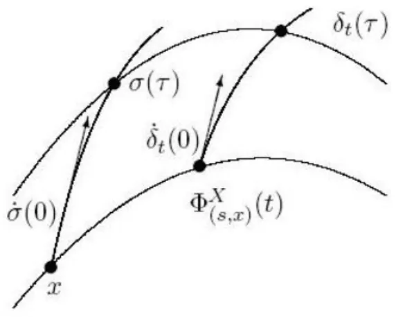
About the geometric meaning of the complete lift
The integral curves ofXT must be understood as the linear approximation of the integral curves ofXwhen the initial condition varies along a curve inM. This idea will appear again in Chapter 4.
Let us explain Figure 2.1. Given an integral curve ofXwith initial condition(s, x), we con-sider a curveσstarting at the pointxof the integral curve. Every point ofσcan be considered as the initial condition at timesfor an integral curve ofX. Thus the flow ofXtransports the curveσat a different curveδtpoint by point. The resultant curve is related with the complete
lift ofXas the following results prove.
Proposition 2.2.4. LetX: I ×M → T M be a time–dependent vector field with evolution operatorΦX and(s, x) ∈I ×M. For > 0, letσ: (−, ) ⊂
R→ M be aC∞curve such
thatσ(0) =x= ΦX(s, s, x). For everyt∈I, consider the curve
δt: (−, ) −→ M
τ 7−→ δt(τ) = Φ(Xs,σ(τ))(t).
18 2.2. Time–dependent vector fields (Proof) ˙ δt(0) = (T0δt(τ)) d dτ 0 =T0 ΦX(s,σ(τ))(t) d dτ 0 =T0 ΦX(t,s)(σ(τ)) d dτ 0 = Tσ(0)ΦX(t,s) T0(σ(τ)) d dτ 0 =Tσ(0)ΦX(t,s)( ˙σ(0)) =TxΦ X (t,s)( ˙σ(0)).
Observe that the curveδtsatisfies the following properties
1. δs(τ) =σ(τ), and
2. δt(0) = ΦX(s,x)(t).
Corollary 2.2.5. LetXbe a time–dependent vector field onM. Forx∈M,v∈TxMand for
> 0, letσ: (−, )⊂R→M be aC∞curve such thatσ(0) =xandσ˙(0) =v. Ifδ
tis the
curve defined in Proposition 2.2.4, thenδ˙(·)(τ) : I → T M,t 7→ δ˙t(τ)is the integral curve of
XT with initial condition(s,σ˙(τ)).
(Proof) The proof just comes from Propositions 2.2.3 and 2.2.4 and the definition of the curveδt.
2.2.2.2 Cotangent lift
Given(t, s)∈I×I, the evolution operatorΦX defines the following diffeomorphism onT M TΦX(t,s):T M −→T M,
which is a linear isomorphism on the fibers onT M. We consider the mapping
Λ(t,s):T∗M −→T∗M (2.2.7)
to be the inverse of the transpose ofTΦX(t,s) on every fiber ofT∗M; that is, forp ∈Tx∗M and
v∈TΦX (t,s)(x)M, Λ(t,s)(x, p) ΦX(t,s), v= p,TxΦX(t,s) −1 (v) = p, TΦX (t,s)(x) ΦX(t,s) −1 (v) .
The mappingΛ :I×I×T∗M →T∗M,Λ(t, s,(x, p)) = Λ(t,s)(x, p), is the evolution operator
of a vector field onT∗M called the cotangent lift ofX and denoted by XT∗. The intrinsic expression of the flow ofXT∗ is given by
Λ(t, s,(x, p)) = ΦX(t, s, x),τTxΦX(t,s) −1 (p) , where τT xΦX(t,s) −1
In local coordinates(x, p)forT∗M, XT∗(t, x, p) =XtT∗(x, p) =Xi(t, x) ∂ ∂xi (x,p) − ∂X j ∂xi (t, x)pj ∂ ∂pi (x,p) .
The equations satisfied by the integral curves of the cotangent lift in the fibers are theadjoint variational equations on the cotangent bundle for X. In the literature, they are sometimes calledadjoint equations forX.
2.2.2.3 A property for the complete and cotangent lift
The previous propositions allow us to determine an invariant function along integral curves ofX.
Proposition 2.2.6. LetX:I×M →T M be a time–dependent vector field and letXT:I×
T M → T T M andXT∗:I ×T∗M → T T∗M be the complete lift and cotangent lift ofX, respectively. Ifγ:I →Mis an integral curve ofXwith initial condition(s, x),V:I →T M
is the integral curve ofXT with initial condition(s, v)wherev∈T
xM, andΛ : I →T∗M is
the integral curve ofXT∗with initial condition(s, p)wherep∈Tx∗M, then
hΛ, Vi:I → R
t 7→ hΛ(t), V(t)i
is constant alongγ.
(Proof) IfΦX is the evolution operator ofX, the evolution operators ofXT andXT∗ are
ΦXT(t, s,(x, v)) = ΦX(t, s, x), TxΦX(t,s)(v) , ΦXT ∗ (t, s,(x, p)) = ΦX(t, s, x), τT xΦX(t,s) −1 (p) ,
respectively, because of Proposition 2.2.3 and§2.2.2.2. Hence
hΛ(t), V(t)i = τT xΦX(t,s) −1 (p), TxΦX(t,s)(v) = τ TxΦX(t,s) −1 (p), TxΦX(t,s)(v) = p, TxΦX(t,s) −1 ◦TxΦX(t,s) (v) =hp, vi= constant.
2.3
Symplectic geometry
LetMbe a smooth manifold andΩ∈Ω2(M). Givenx∈M, the kernel ofΩatxis defined by
20 2.3. Symplectic geometry
which is a subspace of the tangent spaceTxM. It is said thatΩisregularif the dimension of
ker Ωdoes not depend on the pointx∈M. Under the assumption of regularity ofΩ,
ker Ω = [
x∈M
ker Ωx
is a vector subbundle of the tangent bundleT M; that is, a regular distribution onM. The set of all the vector fieldsX ∈X(M)such thatX(x)∈ker Ωxfor allx∈M is also denoted by
ker Ω. The vector subbundleker Ωis involutive if and only ifΩis a closed form.
2.3.1 Symplectic manifolds
A symplectic manifold is a pair(M,Ω) where M is a m–dimensional manifold and Ω is a closed non–degenerate2–form onM. Note that to have a symplectic manifold, the dimension ofM must be even. For instance, the cotangent bundle has associated a symplectic structure.
The non–degeneracy of Ω guarantees that Ω[: X(M) → Ω1(M), defined by the inner productΩ[(X) =iXΩ, is aC∞(M)–module isomorphism. The inverse ofΩ[isΩ]. These two
mappings are the so–calledcanonical musical isomorphisms. TheHamiltonian vector fieldXf
on M associated withf ∈ C∞(M) isXf = Ω](df), whered : Ωs(M) → Ωs+1(M) is the
exterior derivative.
A vector fieldXonMislocally HamiltonianifΩis invariant under the vector field; that is,
LXΩ = 0, whereLis the Lie derivative with respect toXof any tensor field. The invariancy ofΩunderX implies that the1–formiXΩis closed and, by Poincar´e’s Lemma, it is locally
exact.
Aregular Hamiltonian systemis given by(M,Ω, α)where(M,Ω)is a symplectic manifold andαis a closed1–form onM. Poincar´e’s Lemma guarantees that givenx ∈M there exists an open neighbourhoodW ofxandH ∈ C∞(W) such thatα|W = dH. Then,(W,Ω, H)is
called alocally Hamiltonian system. Ifα is an exact form, thenα = dH andHis called the global Hamiltonian function. Thus, a regular Hamiltonian system is given by(M,Ω, H)and is associated with Hamilton’s equationiXHΩ = dHthat always has a unique solution under the
hypothesis of symplecticity.
A natural way to define a Hamiltonian system on the cotangent bundleT∗M is by means of a vector fieldX onM. We takeHX:T∗M → R,HX(px) = hp, X(x)iwithp ∈ Tx∗M,
as a Hamiltonian function to obtain the Hamiltonian system(T∗M,Ω, HX), withΩbeing the
natural 2–form onT∗M. The corresponding Hamiltonian vector field is the cotangent lift of
X defined in §2.2.2.2, as proved in [Barbero-Li˜n´an and Mu˜noz Lecanda 2008b]. This proof follows analogously to the proof of Proposition 2.2.3.
2.3.2 Presymplectic constraint algorithm
The Dirac–Bergmann theory of constraints developed in the fifties for quantum field theory gave rise to the presymplectic constraint algorithm, which has been already adapted and used to
![Figure 4.1: Elementary perturbation of u specified by the data π 1 and the integral curve on M of X {u[π s1 ]} .](https://thumb-us.123doks.com/thumbv2/123dok_us/10922311.2981169/67.892.163.746.576.736/figure-elementary-perturbation-specified-data-π-integral-curve.webp)