Connections
C R McInnes, T J Waters
Department of Mechanical Engineering, University of Strathclyde, Glasgow, G1 1XJ, UK
E-mail: [email protected]
Abstract. Structures are traditionally designed to be stable. However, unstable configurations (such as buckling) can in principle be controlled in smart structures using embedded sensors and actuators. In this paper we explore a new means of reconfiguring smart structures by connecting multiple unstable configurations. Methods from dynamical systems theory are used firstly to identify sets of unstable configurations in a simple smart structure model, and then to connect them through so-called heteroclinic connections in the phase space of the problem. The instability inherent in the structure is then actively utilised to provide an effective new way of transitioning between configurations of the structure in a controlled manner.
1. Introduction
Smart structures offer the possibility of active control of mechanical systems through the use of embedded sensors and actuators. Applications range from active vibration control of small amplitude displacements through to active shape control at large deformations (e.g. [1, 2, 3]). Other more ambitious applications include improving the buckling limit of beams under compressive load. For active control of buckling, continuous sensing and actuation is required to ensure the integrity of the structure past the classical, critical buckling limit. In such applications computational effort replaces mechanical strength. The embedded controller must then cope with potentially violent instability, as opposed to small amplitude displacements for vibration control (e.g. [4, 5]).
The active control of unstable smart structures has been investigated by Hogg and Huberman using an agent-based approach to suppress instability [6]. These ideas were extended by Guenther et al. to consider the possible benefits of transitions between unstable states, relative to transitions between stable states [7, 8]. Using relatively simple, but qualitatively interesting models, these investigations provide new insights into the dynamics of unstable smart structures. In particular, the concept of exploiting instability is raised as a means of reducing the energy requirements for transitions
between configurations of the structure. Numerical experiments demonstrated a
phase space connections from modern dynamical systems theory [9]. Firstly, a set of equilibrium configurations will be identified in a simple model of a reconfigurable smart structure. A reconfigurable smart structure is defined here as a mechanical system which has the ability to change its kinematic configuration between a finite set of equilibria (stable or unstable). It will be assumed that the simple reconfigurable structure used later possesses embedded sensors and actuators which will allow the structure to be actively controlled. In particular, it will be assumed that the structure can be stabilised at naturally unstable equilibria through the use of active control. It will then be shown that a subset of unstable, equal energy configurations can be connected, allowing highly efficient reconfiguration of the entire structure. The development of this central idea will exploit aspects of modern dynamical system theory, which again will be illustrated using a simple, representative model of an unstable smart structure. It is our intention in this paper to introduce and explore a new concept, rather than provide a detailed analysis using a high fidelity model of a real structure.
In general, non-linear dynamical systems typically posses a number of equilibria which may be connected through paths in the phase space of the system. In particular, equilibria with both stable and unstable manifolds may be connected through so-called heteroclinic connections [9]. Here, a manifold is defined as a surface embedded in phase space. The unstable manifold then represents the family of trajectories diverging from an equilibrium point, while the stable manifold represents the family of trajectories asymptotically approaching an equilibrium point. A heteroclinic connection is formed if the unstable manifold of an equilibrium point intersects the stable manifold of another distant equilibrium point in phase space. These phase space structures have important applications in diverse fields such as mechanics [10], astrodynamics [11] and fluids [12]. More complex phase space structures, termed heteroclinic networks, can then be formed from an assembly heteroclinic connections [13].
Heteroclinic connections will investigated here as a rigorous means of enabling transitions between unstable configurations of a reconfigurable smart structure. For a real mechanical system, heteroclinic connections will correspond to phase space trajectories whose projection into configuration space connects the unstable configurations (equilibria) of the structure. As will be seen, unstable equilibria can be found which lie on the same energy surface in phase space. Therefore, if heteroclinic connections between unstable, equal energy equilibria can be identified, trajectories exist between these configurations which in principle do not require the addition of or dissipation of energy. The intersection of invariant manifolds in phase space can then be used as a novel means of connecting different, equal energy unstable configurations, leading to highly efficient reconfiguration of the structure. We note here that compliant structures with multiple equilibria have been investigated for some time, but that unstable equilibria are largely ignored, with only transitions between stable equilibria deemed important (e.g. [14, 15]).
equilibria can in principle be extremely efficient compared to reconfiguring a structure between stable configurations. A transition between stable configurations requires the input of, and then dissipation of energy to cross the potential barrier separating the stable equilibria. The work done to cross the barrier requires the input of energy, while the subsequent dissipation of that energy to reach the new stable equilibrium
generates waste heat. In comparison, the use of heteroclinic connections between
unstable, equal energy equilibria only requires that the effect of dissipation during the reconfiguration process is compensated for. This dissipation is a path integral along the heteroclinic connection through phase space, and can be overcome using a suitable controller. Clearly, the energy required to actively control the instability must also be sufficiently small for the concept to be of benefit. However, for frequently actuated devices the accumulated work done in reconfiguring between stable equilibria will be significant, while the duration the system spends in active control at unstable equilibria will be small. Further work will investigate this issue in detail.
Potential applications of the phase space connection concept include use in MEMS-type devices which require frequent switching of compliant components to reduce mean power consumption and waste heat dissipation. For example, previous work has demonstrated the existence of multiple equilibria in MEMS cantilevered beams [16] and torsional devices [17] with electrostatic forces, while MEMS-scale bistable beam mechanisms have been fabricated [18]. On a more speculative level, switched nano-mechanical devices have been considered for reversible computing which require frequent, rapid mechanical transitions [19]. Other applications include power reduction in smart structures used in rapidly actuated control surfaces for active flow control and the efficient reconfiguration of large deployable spacecraft antennae [20, 21]. In general, the use of heteroclinic connections between unstable equilibria is likely to be of benefit for power and energy constrained applications, such as aerospace, and for compliant structures requiring frequent reconfiguration, such as MEMS devices.
2. Smart structure model
2.1. Single mass problem
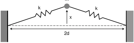
In order to investigate the use of heteroclinic connections to reconfigure unstable smart structures, a simple representative model of a naturally unstable structure will be defined. Firstly, a simple model of a beam under compressive load will be considered. The essential behaviour of the beam can be captured by representing the inertia of the beam as a single lumped mass and the stiffness of the beam by two linear springs. We therefore consider a beam clamped at both ends, as shown in figure 1, represented as
a mass m connected to two linear springs of stiffness k and natural length l. If the
displacement of the mass is defined by x, (such that x ≤ √l2
−d2), while the springs
x
[image:4.595.186.402.92.161.2]2d
Figure 1. 1 degree-of-freedom buckling beam model comprising a single lumped massm with spring constantkand displacementxfrom (unstable) equilibrium. The springs are pinned at both ends and the displacement is assumed to be constrained to the vertical.
˙
x=v (1)
mv˙ =−2kx
Ã
1−√ l
x2+d2
!
(2)
The non-linear term in equation (2) can be expanded by assuming x/d≪1 to obtain
˙
x=v (3)
mv˙ = 2k
Ã
l d −1
!
x− kl d3x
3
+. . . (4)
Then, a non-dimensional position coordinate q = ql/d3x and non-dimensional time
τ =t/qm/k can be defined. In this simple model, the position coordinate q represents
the displacement of the beam from its undeformed state with corresponding momentum coordinatepsuch that (q, p)∈R2
. We note that although equation (4) has been derived
assuming x/d ≪ 1, we will place no restriction on q in the subsequent analysis. The
simple cubic nonlinearity in equation (4) will suffice to provide the required qualitative behaviour in the model, without undue algebraic complexity. The qualitative non-linear model for the beam is therefore defined by
˙
q=p (5)
˙
p=µq−q3
(6)
The free parameterµ= 2(l/d−1) is used as a measure of the compressive load acting on
the beam. Clearly, if the structure is in tension (l < d) then µ <0 while if the structure in in compression (l > d) then µ > 0 with the critical buckling load corresponding to
µ = 0. It can be seen that for µ < 0, equation (6) admits a single real equilibrium
solution ( ˙p = 0) at qe0 = 0 corresponding to an undeflected beam in tension. For
µ > 0, equation (6) admits 3 equilibria defined as qe0 = 0, qe1 = +√µ and qe2 = −√µ,
corresponding to a symmetric buckled configuration. A supercriticial bifurcation then
The change to the qualitative behaviour of the system detailed above can be
seen through the use of an effective potential for the problem V(q, µ) such that
˙
p=−∂V(q, µ)/∂q. The potential can then be defined as
V(q, µ) = −1 2µq
2
+ 1
4q
4
(7)
The change to the number and type of turning points of V(q, µ) can be seen in figure
2, again with the supercriticial bifurcation occurring at µ = 0. For µ < 0 there is a
single global minimum at qe0 defined by ∂V(q, µ)/∂q = 0 with ∂2V(q, µ)/∂q2 >0 while
forµ >0 there are 3 turning points with a local maximum atqe0 with∂2V(q, µ)/∂q2 <0
and local minima at qe1 and qe2 with ∂2V(q, µ)/∂q2 > 0. It is clear that qe0 becomes
unstable when the two new (stable) equilibrium points qe1 and qe2 appear.
The stability properties of the equilibria can also be determined from the eigenvalues
λ which are found from linearisation of equation (6). The eigenvalue spectrum is found
to be ±√µ, ±i√2µ and ±i√2µ for qe0, qe1, and qe2 respectively. Again, it can be seen
that for µ < 0, qe0 is linearly stable (Re(λ) = 0) while for µ > 0, qe0 becomes unstable
(Re(λ) > 0) while the two new equilibria qe1 and qe2 are linearly stable. The onset of
buckling atµ= 0 is again identified as the transition fromqe0to one of the two new stable
equilibria at qe1 or qe2. The supercriticial bifurcation at µ = 0 can then be associated
with buckling at some critical compressive load. The full bifurcation diagram for this single mass problem is shown in figure 3.
Lastly, we note that while equation (6) has similarities to a pitchfork bifurcation, the classical pitchfork bifurcation is in fact defined for first order systems [22]. However, with strong dissipation (over-damped system) equation (6) can be transformed to first
order. Adding linear dissipation parameterised by β, equation (6) becomes
˙
q=p (8)
˙
p=µq−q3
−βp (9)
Then, ifβ ≫1, equation (9) reduces to the first order equation ˙q= (1/β)(µq−q3
), which has the same equilibria as equation (6) and represents a classical pitchfork bifurcation. Physically, this represents a rapid transition to the buckled state after the bifurcation. With modest dissipation added to the second order system in equation (9), the stable equilibriaqe1 andqe2 are no longer centres with purely imaginary eigenvalues, but spirals
with complex eigenvalues with negative real part. The effect of dissipation on the reconfiguration problem presented here will be discussed later.
2.2. Chain of coupled masses
We now consider a coupled problem with a chain ofN masses, using the same functional
Μ=1
Μ=0.5
Μ=-1
-2 -1 0 1 2
-0.3
-0.2
-0.1 0.0 0.1 0.2
q
[image:6.595.188.404.90.298.2]V
Figure 2. Effective potentialV(q, µ) for a 1 mass chain with a single lumped mass. Single equilibriumqe0 forµ <0 with two new equilibriaqe1 andqe2 appearing after the
supercriticial bifurcation atµ= 0.
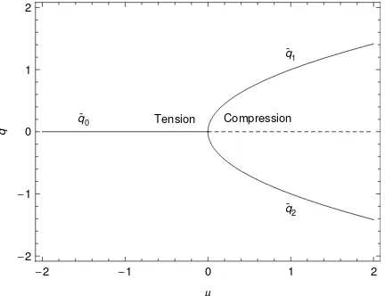
q0
q1
q2 Tension Compression
-2 -1 0 1 2
-2
-1 0 1 2
Μ
q
Figure 3. Bifurcation diagram for a 1 mass chain for−2≤µ≤2, solid line: stable equilibria (Re(λ) = 0), dashed line: unstable equilibria (Re(λ)>0). The equilibrium at eq0= 0 becomes unstable forµ >0, creating stable equilibriaeq1 andqe2.
unstable structure [6, 7, 8]. It will be assumed at first that the dynamics of the problem are conservative with no dissipation. The effect of dissipation will be discussed later.
From equation (7), the generation of the potential can be generalised to an arbitrary
pair of neighbouring massesi−1 and i as
V(qi−1, qi, µi) =− 1
2µi(qi−1−qi)
2
+ 1
4(qi−1−qi)
4
(10)
[image:6.595.189.405.374.540.2]that the displacements q1,2 can be sensed and that the coupling parameters µ1−3 can
be manipulated to effect active control over the structure. Manipulating the coupling coefficients is equivalent to manipulating the natural length of the springs in the model. In principle, a spring fabricated from shape memory alloy could posses this property. It can be seen that equation (10) has similarities with the classical problem of oscillations
in a chain of coupled masses [23], but with instability since µi > 0. However, the
interaction of the de-stabilising quadratic term with the stabilising quartic term will yield families of both stable and unstable equilibria.
The global configuration of the unstable structure is now defined by the setq={qi}
(i = 1 −N) with an associated set of momenta p = {pi} (i = 1 − N) such that
(q,p)∈R2N. The behaviour of the chain of masses can be described by a Hamiltonian
H(q,p, µ) =T(p) +V(q, µ) for kinetic energyT(p) and potential V(q, µ) where
T(p) = 1 2kp
2
k (11)
V(q, µ) =
N+1
X
i=1
−12µi(qi−1 −qi)
2
+ 1
4(qi−1−qi)
4
(12)
with the Dirichlet boundary conditions q0 = 0 and qN = 0, so that the chain is pinned
at both ends. The dynamics of the problem (phase flow) are now defined by Hamilton’s equations of the form
˙
q=∇pH(q,p, µ) (13)
˙
p=−∇qH(q,p, µ) (14)
where ∇q = ∂/∂q and ∇p = ∂/∂p. These can be written in compact form using
z= (q,p)∈R2N as
˙z =J · ∇zH(z, µ) (15)
where the symplectic matrixJ is defined by
J = Ã
0 I
−I 0 !
(16)
In general, a set of equilibrium configurations E for equation (15) can be found defined
aszei (i= 1−N). However, since the potential is independent ofp, the setE is obtained
from ∇qV(q, µ) = 0. This condition results in an algebraic equation, the solution of
which which yields the set of equilibria E defined as qei (i = 1− N). In general E
will contain both linearly stable equilibria Es (Re(λ) = 0) and unstable equilibria Eu
(Re(λ)>0) for some eigenvalue spectrum λ.
In general, the linear stability of the set E can be determined through linearisation
of Hamilton’s equations in the neighbourhood of each equilibrium point inE. Defining
a displacementξ from equilibriumezsuch thatξ =z−ze, a Taylor expansion of equation (15) provides
˙
ξ=J· ∇2
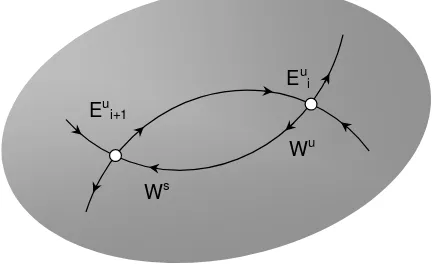
Eui Eui+1
Ws
[image:8.595.186.403.96.228.2]Wu
Figure 4. Heteroclininc connection between two distant equilibria Eu
i and Eui+1 on
the same energy surface in phase space, formed by the intersection of the unstable manifoldWuofEu
i and stable manifoldWsofEiu+1
Then, the eigenvalue spectrum λ of E is found from the resulting characteristic
polynomial obtained from
kJ· ∇2
zH(ez, µ)−λ·Ik= 0 (18)
For the Hamiltonian problem considered here, a set of linearly stable equilibria Es are
expected with conjugate imaginary eigenvalues along with a set of unstable equilibria
Euwith real eigenvalues of opposite sign [9]. These so-called hyperbolic points represent
trajectories in phase space which recede from an equilibrium point along an unstable manifoldWu (Re(λ)>0) or approach an equilibrium point along a stable manifold Ws
(Re(λ) < 0). If the unstable manifold Wu of an equilibrium point Eu
i intersects the
stable manifoldWsof a distant equilibrium pointEu
i+1in phase space, then a heteroclinic
connection exists between the equilibria. In general, if ψ(t) is a phase space trajectory there exists a heteroclinic connection betweenzei and zei+1 if ψ(t)→ezi as t→ −∞ and
ψ(t) → ezi+1 as t → +∞. Here, we are particularly interested in the set of hyperbolic
pointsEu which exist on the same energy surface W in phase space, as shown in figure
4. Heteroclinic connections between these points do not in principle require the addition of or dissipation of energy, with significant practical benefits for reconfiguring the smart structure.
3. Heteroclinic connections
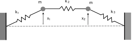
3.1. Two mass chain
x1
m
k 3
x2
m
k 2
[image:9.595.187.403.90.158.2]k1
Figure 5. 2 degree-of-freedom buckling beam model comprising two lumped masses
mwith spring constantsk1,2 and displacementsx1,2 from (unstable) equilibrium. The
springs are pinned at both ends and the displacement is assumed to be constrained to the vertical.
T(p) = 1 2(p
2 1+p
2
2) (19)
V(q, µ) = − 1 2µ1q
2 1 −
1
2µ2(q1−q2)
2
− 12µ3q 2 2 + 1 4q 4 1 (20) + 1
4(q1−q2)
4
+1
4q
4 2
The dynamics of the chain are then obtained from Hamilton’s equations, where now (q,p) ∈ R4
. However, since the kinetic energy is clearly independent of q, it can be
seen from equation (14) that the dynamics are described by ˙p=−∇qV(q, µ) so that
˙
q1 =p1 (21)
˙
p1 =µ1q1−q 3
1 +µ2(q1−q2)−(q1−q2) 3
(22) ˙
q2 =p2 (23)
˙
p2 =µ3q2−q 3
2 −µ2(q1−q2) + (q1−q2) 3
(24)
Calculating the gradient of the potential such that ∇qV(q, µ) = 0, yields two
simultaneous algebraic equations whose solution defines the set of equilibriaE. However,
from equations (22) and (24) it can be seen immediately that
˙
p1+ ˙p2 =q1(µ1−q 2
1) +q2(µ3−q 2
2) (25)
so that we expect equilibria at (0,0), (√µ1,√µ3) and (−√µ1,−√µ3). However, when
the coupling constants are equal, such that µ1−3 = µ, the equilibria merge to form a
continuous ring defined by µ(q1+q2)−(q 3 1+q
3
2) = 0. This rotational symmetry is then
broken forµ2 > µ1 to form 5 equilibria, as will be discussed later. Also, since in general
˙
p1+ ˙p2 6= 0, the total momentum of the system is not conserved. While the total energy
is conserved, the absence of another integral of motion for such a 2-degree-of-freedom system suggests that the system is not integrable.
Solving ∇qV(q, µ) = 0 yields five equilibria for µ1−3 > 0. The location of the
equilibria are listed in table 1 for µ1 = 1, µ2 = 1.5 and µ3 = 1 along with the eigenvalue
maximum, 2 unstable equilibriaE1 andE2 where the potential has a saddle and 2 stable
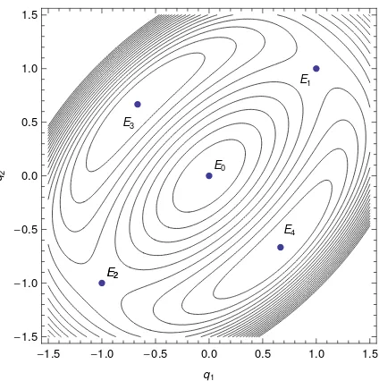
equilibriaE3 andE4 where the potential has a global minimum, as can be seen in figure
6. The corresponding shape of the structure associated with each of these 5 equilibrium
configurations shown in figure 7. It can be seen from table 1 that E0 has the highest
potential V, corresponding to the two masses being undeflected, with both springs in
compression. E1 and E2 then have equal potential which is higher than E3 and E4.
For the unstable equilibria E1 and E2, only the central spring is in compression and
can in principle relax to the lower energy equilibria at E3 and E4 where both springs
are extended. We note that since the Hamiltonian H = T(p) +V(q, µ) is constant,
the volume of phase space in R4
, and its projection to configuration space in R2
, is
constrained by the requirement that T(p)≥0.
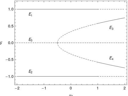
It can be shown that the stability properties of the equilibria are a function of the coupling parameters µ1−3. In particular, the stability properties of E1,2 and E3,4 swap for µ2 > µ1, as will be seen later. It can also be shown that the location of E1 and E2
are independent of µ2 while the location of E3 and E4 is a function of µ2. Therefore,
fixing µ1 and µ3, a bifurcation diagram can be constructed. Although only µ1−3 > 0
is considered in the subsequent analysis, for completeness the bifurcation diagram is shown for −2 ≤µ2 ≤2 in figure 8. It can be seen that the stability properties of E1,2
and E3,4 swap for µ2 > µ1, as noted above.
Since the unstable equilibria E1 and E2 lie on the same energy surface, if a
heteroclinic connection can be found between E1 and E2 the structure can in principle
be reconfigured from E1 to E2 without working being done, again in the absence of
dissipation. The change in energy for the reconfiguration δV =V(qe1)−V(qe2)≈ 0. If
the structure in figure 6 is at the stable equilibrium E3, it can transition to the other
stable equilibrium at E4 only by crossing the potential barrier at E1. Therefore, the
change in energy for reconfiguration to E4 is δV =V(qe3)−V(qe1) ≈ −0.39, assuming
that the energy input to cross the potential barrier at E1 is dissipated to finally reach
E4. If frequent reconfigurations of the structure are required, it is clear that the use of
heteroclinic connections between unstable equilibria may be significantly more efficient. We note however, that work is in principle required required to stabilise the structure
when operating at the unstable configuration at E1. However, by exploiting the change
in stability properties ofE1 andE2 close toµ2 =µ1 it will be possible to provide passive
stability to E1 and E2, as will be discussed later.
In order to explore possible connections between these unstable equilibria, their stable and unstable manifolds must be investigated. Firstly the eigenvectors associated with each eigenvalue are found. For the 2 unstable equilibriaE1 andE2 there exists pair
of real eigenvalues of opposite sign. Associated with these eigenvalues are eigenvectors
us
and uu
corresponding to the eigenvalues λ = −1 and λ = +1 respectively. These
eigenvectors are tangent to the stable manifold Ws and the unstable manifold Wu
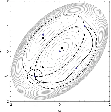
E0 E1 E2 E2 E3 E4
-1.5 -1.0 -0.5 0.0 0.5 1.0 1.5
[image:11.595.191.403.84.297.2]-1.5 -1.0 -0.5 0.0 0.5 1.0 1.5 q1 q2
Figure 6. Effective potential V(q, µ) for a two mass chain with µ1 = 1, µ2 = 1.5
and µ3 = 1 yielding 5 equilibria (3 unstable equilibria E0, E1 and E2, and 2 stable
equilibriaE3andE4).
[image:11.595.187.407.374.571.2]E0 -1.5 -1.0 -0.5 0.0 0.5 1.0 1.5 q E1 -1.5 -1.0 -0.5 0.0 0.5 1.0 1.5 q E2 -1.5 -1.0 -0.5 0.0 0.5 1.0 1.5 q E3 -1.5 -1.0 -0.5 0.0 0.5 1.0 1.5 q E4 -1.5 -1.0 -0.5 0.0 0.5 1.0 1.5 q
Figure 7. Equilibria for a two mass chain with unstable equilibria E0, E1 and E2
and stable equilibria E3 andE4. The unstable symmetric pairE1 and E2 have equal
potential V.
Table 1. Stability properties of the 5 equilibria of a two mass chain with µ1 = 1,
µ2= 1.5 andµ3= 1
Point eq1 eq2 λ1,2 λ3,4 V Type
E0 0 0 ±1 ±2 0 Saddle×Saddle
E1 1 1 ±
√
2i ±1 −1/2 Saddle×Centre
E2 −1 −1 ±
√
2i ±1 −1/2 Saddle×Centre
E3 −2/3 2/3 ±1/
√
3i ±2√2i −8/9 Centre×Centre
E4 2/3 −2/3 ±1/
√
[image:11.595.143.454.681.758.2]E0
E1
E2
E3
E4
-2 -1 0 1 2
-1.0
-0.5 0.0 0.5
Μ2
q
[image:12.595.190.404.87.248.2] 1
Figure 8. Bifurcation diagram for a two mass chain. Projection of the location of the equilibria onto theq1 axis forµ1= 1,µ3 = 1 and−2≤µ2 ≤2, solid line: stable
equilibria (Re(λ) = 0), dashed line: unstable equilibria (Re(λ)>0).
phase space with initial conditions
zs=ze±ǫus (26)
zu =ze±ǫuu (27)
for ǫ ≪ 1. If the manifolds intersect then a heteroclinic connection will exist between
the equilibria and the structure can be reconfigured by transitioning between the two unstable statesE1 and E2.
3.2. Uncontrolled heteroclinic connection
The search for heteroclinic connections discussed above is aided by the presence of symmetry in the problem. Indeed, symmetry is often an essential requirement for the existence of heteroclinic connections in dynamical systems. We will therefore impose
symmetry on the problem by setting µ3 =µ1. We then note from equations (22) and
(24), and indeed from figure 6, that the system then admits the symmetries γ1 and γ2
defined by
γ1 :
Ã
q1
q2
!
→
Ã
q2
q1
!
γ2 :
Ã
q1
q2
!
→
Ã
−q2
−q1
!
(28)
which amount to reflections through q2 = q1 and q2 = −q1 respectively. Since γ1 and
γ2 form a group Γ, the problem forms a so-called equivariant dynamical system [13].
Then, given that the dynamics of the problem are defined by ˙p=−∇qV(q, µ), it can be
shown that∇qV(γ.q, µ) =γ.∇qV(q, µ) forγ ∈Γ. This property of the system ensures
that once a solution q(t) is found, symmetric solutions can also be found using γ1 and
γ2. Therefore, any solution generated fromq(t) ={γ.q(t)|γ ∈Γ}is also a valid solution
To take advantage of these symmetries the coordinate axes (q1, q2) will be rotated
anticlockwise by π/4 with the following coordinate transformation
Ã
q1
q2
! = √1
2 Ã
1 −1
1 1 ! Ã Q1 Q2 ! (29)
Then, the potential defined in equation (20) can be transformed to
V(Q, µ) = 1 8(Q
4 1+Q
2 1(6Q
2
2−2(µ1+µ3)) + 4Q1Q2(µ1−µ3) (30)
+Q2 2(9Q
2
2−2(µ1+ 4µ2+µ3)))
In this new coordinate system, the equations of motion can be obtained from ˙P =
−∇QV(Q, µ). The dynamics are then described by
˙
Q1 =P1 (31)
˙
P1 =−
Q1
2 (Q
2 1+ 3Q
2
2−2µ1), (32)
˙
Q2 =P2 (33)
˙
P2 =−
Q2
2 (3(Q
2 1+ 3Q
2
2)−2µ1−4µ2) (34)
In this form the equilibria can again be located (withµ1,2 >0). It can be shown that the
origin E0 is a double saddle with eigenvalues ±√µ1, ±√µ1+ 2µ2 while E1 and E2 are
located at (±√2µ1,0) and have eigenvalues±i√2µ1,±
q
2(µ2−µ1). Finally,E3 andE4
are located at (0,±1 3
q
2(µ1+ 2µ2)) with eigenvalues ±i
q
2(µ1+ 2µ2), ±
q
2
3(µ1−µ2).
The eigenvalues are again obtained by linearisation of equations (32) and (34) at the appropriate equilibrium point.
Using the transformed coordinates, it can be seen that E3 and E4 will merge with
E0 for µ2 < −21µ1, as shown in figure 8. Similarly, it is clear that the sign of µ1 −µ2
determines the stability of the equilibria, with a bifurcation taking place as µ1 −µ2
crosses zero. Here a pair of conjugate imaginary eigenvalues become real, leading to a transition for a centre to a saddle. Therefore, when µ1 < µ2, the equilibria E1,2
are unstable (saddle × centre) and E3,4 are stable (centre × centre). When µ1 > µ2
these stability properties are reversed, again shown in figure 8. When µ1 = µ2, the
system admits a ‘ring equilibrium’, as noted earlier. For the numerical investigations that follow, we will let µ2 > µ1, as in this case E1,2 are unstable and their position is
independent ofµ2.
In the rotated coordinates, the system is symmetric about the axes Q1 = 0 and
Q2 = 0. The unstable manifold of E1, for example, is then the reflection of the stable
manifold of E2. Therefore, a heteroclinic connection between E1 and E2, if one exists,
must be symmetric about theQ2axis, and so must intersect Q1 = 0 perpendicularly, i.e.
˙
Q2 = 0, as shown in figures 9 and 10. The numerical method used to find heteroclinic
E1
E2
-2 -1 0 1 2
0.0 0.5 1.0
Q1
Q2 E1,2
-2.0 -1.5 -1.0 -0.5 0.0
-1.0
-0.5 0.0 0.5 1.0
P1
[image:14.595.152.441.95.233.2]P2
Figure 9. A heteroclinic connection between E1 at (2,0) and E2 at (-2,0) for
µ1 = 2, µ2 = 1.68 µ1 and µ3 = 2. The projection of the phase space path into
configuration space Q and momentum space P is shown. Note the perpendicular crossing ofQ1= 0 with ˙Q2= 0.
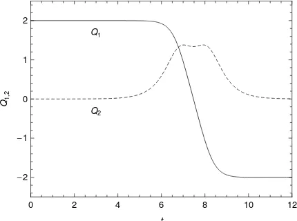
Q1
Q2
0 2 4 6 8 10 12
-2
-1 0 1 2
t
Q1
,2
Figure 10. Transformed coordinatesQ1andQ2for a heteroclinic connection between
E1at (2,0) andE2 at (-2,0) forµ1= 2, µ2= 1.68µ1 andµ3= 2.
equations in the direction of the unstable eigenvector of E1 as in equation (27), until
it intersects the Q2-axis, i.e. Q1 = 0. We measure ˙Q2 at this time, and if ˙Q2 = 0
(or less than some cut-off) a heteroclinic connection exists between E1 and E2 for this
parameter set. Due to symmetry, a heteroclinic connection will also exist between E2
and E1, and both connections will have a mirror image under Q2 → −Q2. This is a
consequence of the dynamics of the problem being equivariant.
As noted earlier, a true heteroclinic path is an asymptotic connection. It therefore
reaches the equilibrium points as t → ±∞. This is clearly impractical for a real
structure. Therefore, we must instead approximate the true heteroclinic paths with approximate heteroclinic paths, by which we mean the path enters the close vicinity of both fixed points in finite time. For this reason, we do not require ˙Q2 to be exactly zero
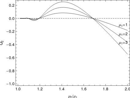
[image:14.595.187.402.325.485.2]Μ1=1
Μ1=2
Μ1=3
1.0 1.2 1.4 1.6 1.8 2.0
-1.0
-0.8
-0.6
-0.4
-0.2 0.0 0.2
Μ2Μ1
Q
[image:15.595.190.402.88.248.2]2
Figure 11. The value of ˙Q2at the first crossing of the unstable manifold of E1with
theQ2 axis, with increasing parameter ratioµ2/µ1.
From the transformed equations of motion it can again be seen that when µ1 =µ2
there is a continuous ring of equilibria which, from equations (32) and (34), is the ellipse defined byQ2
1+3Q 2
2 = 2µ. Forµ2 > µ1the symmetry of this continuous ring of equilibria
is broken into the four equilibria E1−4. Once this symmetry is broken the connection
between E1 and E2 can persist in the form of a heteroclinic connection. Numerically,
it is found that forµ2 <1.2µ1, ˙Q2 is sufficiently small for an approximate heteroclinic
path to exist, as shown in figure 11. Then, whenµ2 ≈1.68µ1, a heteroclinic path exists,
irrespective of the value of µ1, as is clearly seen in figure 11. This demonstrates that
for each value of µ1 there is a value of µ2 not close to µ1 which admits a heteroclinic
path. Lastly, instead of measuring the value of ˙Q2 on the first intersection withQ1 = 0,
we could instead continue the integration until subsequent intersections. We find that
there are more complicated heteroclinic paths which leave E1, intersect the Q2 axis
a number of times, and then approach E2. While these paths are of interest, their
more complicated form suggests they are more likely to be destroyed by damping or parameter inaccuracy, and so will not be discussed further here. We may conclude that exact heteroclinic paths do not exist for every choice of parametersµ1 and µ2. However,
we can overcome this shortcoming by using a controller, which we shall discuss in the next section.
3.3. Controlled heteroclinic connection
It has been shown that the 2 mass chain admits families of heteroclinic connections in the phase space of the problem. These families of trajectories rely on both the symmetry and the Hamiltonian structure of the dynamics. For a more realistic model however, dissipation must be considered, which will of course destroy the Hamiltonian structure
of the dynamics. Therefore, phase trajectories emerging from E1 will not reach E2. To
operation at E2 following the transition.
The dynamics of the problem will now be extended by the addition of linear dissipation parameterised by β. Then, returning to the original variables (q1, q2) for
ease of illustration, the dynamics are defined by
˙
q1 =p1 (35)
˙
p1 =µ1q1−q 3
1 +µ2(q1−q2)−(q1−q2) 3
−βp1 (36)
˙
q2 =p2 (37)
˙
p2 =µ3q2−q 3
2 −µ2(q1−q2) + (q1−q2) 3
−βp2 (38)
It can then be shown that in general (p1 6= 0, p2 6= 0) the total energy W = T +V of
the system is monotonically decreasing such that ˙W =−β(p2 1 +p
2
2). In order to define
a suitable controller it will be assumed that the statesq= (q1, q2) and p= (p1, p2) can
be observed. Similarly, in order to effect control, it will be assumed that the coupling
parameters µ1−3 can be manipulated. This is equivalent to manipulating the natural
length of the springs in the model. As will be seen, the system is controllable through the manipulation of µ1 and µ3 only, with µ2 fixed.
In order to ensure convergence to some equilibrium point (qe1,qe2) a Lyapunov
function [24] will be defined as
φ(q,p) = 1
2(p1+p2)
2
+1
2(q1−qe1)
2
+1
2(q2−qe2)
2
(39)
where φ(q,p) > 0 and φ(0,0) = 0. The time derivative of the Lyapunov function is clearly
˙
φ(q,p) =p1( ˙p1+ (q1−qe1)) +p2( ˙p2+ (q2−qe2)) (40)
Then, substituting from equations (36) and (38) the following controllers for µ1 and µ3
can be defined (q1,2 6= 0) as
µ1 =−
1
q1
((q1−qe1) +ηp1+q1−q 3
1+µ2(q1−q2) + (q1−q2) 3
) (41)
µ3 =−
1
q2
((q2−qe2) +ηp2+q2−q 3
2−µ2(q1 −q2) + (q1 −q2) 3
) (42)
for some control parameter η. It can be seen that φ is monotonically decreasing such
that
˙
φ(q,p) = −(η+β)(p2 1+p
2
2)¹0 (43)
and so q −→ (qe1,qe2) and p −→ (0,0) within the neighbourhood R of E2. If the
neighbourhood R of E2 is sufficiently small, it can also be shown that the controls can
E0
E1
E2
E3
E4
R
S
-2 -1 0 1 2
-2
-1 0 1 2
[image:17.595.190.403.90.304.2]q1 q2
Figure 12. Controlled transition fromE1at (1,1) toE2 at (-1,-1) with the controller
active in the neighbourhood R of E2 (dissipation parameter β = 0.01). Contour S
represents the allowed region of motion withT(p)>0.
δµ1 =
1 2δq1−
3
2δq2+ηp1 (44)
δµ3 =−
3 2δq1+
1
2δq2+ηp2 (45)
where (δq1, δq2) = (q1 −qe1, q2 −qe2). We note from equation (43) that ˙φ(q,p) is only
rendered negative semi-definite and so asymptotic stability withinRis not ensured from
equation (43) alone. However, the Krasovskii-LaSalle principle [24] can be invoked to demonstrate asymptotic stability. It can be seen that both φ(0,0) = 0 and ˙φ(0,0) = 0. In addition the set {(q,p)|φ˙(q,p) = 0} does not contain any trajectory of the system, except the trivial trajectoryq=p= 0 withinR, so that asymptotic stability is ensured. An example of a controlled heteroclinic connection forµ1 = 1, µ2 = 1.5 andµ3 = 1
is shown in figure 12 (β = 10−2). In the absence of dissipation, the Hamiltonian
H = T(p) + V(q, µ) is constant so that the volume of phase space in R4
, and its projection to configuration space inR2
, is constrained by the requirement thatT(p)≥0, identified by contour S in figure 12. Since the ratio ofµ1 and µ2 is not close to 1.68, an
exact heteroclinic connection will not occur (in the absence of dissipation), as can be seen from figure 11. To initiate the heteroclinic connection, a displacement along the
unstable manifold of E1 is performed (ǫ= 10−
4
) and the controller activated when the
phase path is in the neighbourhood R of E2 (η = 2). The corresponding shape of the
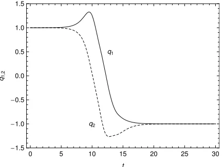
structure during the transition from E1 toE2 is shown in figure 13.
The heteroclinic connection can also be seen in figure 14, where the controller
-1.5
-1.0
-0.5 0.0 0.5
-1.5
-1.0
-0.5 0.0 0.5
t=10
-1.5
-1.0
-0.5 0.0 0.5 1.0 1.5
t=12
-1.5
-1.0
-0.5 0.0 0.5 1.0 1.5
t=14
-1.5
-1.0
-0.5 0.0 0.5 1.0 1.5
t=30
-1.5
-1.0
[image:18.595.187.406.92.292.2]-0.5 0.0 0.5 1.0 1.5
Figure 13. Controlled transition from unstable equilibrium E1 at t=0 to unstable
equilibriumE2 att=30.
q1
q2
0 5 10 15 20 25 30
-1.5
-1.0
-0.5 0.0 0.5 1.0 1.5
t
q1,2
Figure 14. Mass displacements during the transition formE1at (1,1) toE2at (-1,-1).
shown in figure 15. It can be seen that the controls are only active when the phase
path is within region R of E2 and that a smooth control time history is achieved.
Numerical experiments demonstrate that the integrated control effort grows with
increasing dissipation parameter β. Indeed, increasing β, the region R needs to be
enlarged to ensure capture of the phase path at E2, as shown in figure 16. In addition,
the duration of the reconfiguration manoeuvre can be reduced by providing a larger
displacementǫalong with unstable eigenvector of E1 defined in equation (27), as shown
[image:18.595.189.406.353.516.2]Μ1
Μ3
0 5 10 15 20 25 30
1.00 1.02 1.04 1.06 1.08 1.10 1.12
t
Μ1
[image:19.595.191.403.88.246.2],3
Figure 15. Controls in region R in the neighbourhood of E2 actuated through the
coupling parametersµ1 andµ3withη= 2.
E0
E1
E2
E3
E4 Β=0.01
Β=0.1
-2 -1 0 1 2
-2
-1 0 1 2
q1 q2
Figure 16. Controlled transition fromE1at (1,1) toE2at (-1,-1) with the controller
active in the neighbourhoodR ofE2 (dissipation parameterβ= 0.01,β= 0.1).
3.4. Bifurcation control
As note earlier, although the use of heteroclinic connections appears attractive, work
is required to stabilise the structure when operating in the unstable configurations E1
and E2. However, this limitation may be overcome if the free parameters µ1−3 are
selected such that the structure is operating near the critical region of the bifurcation diagram in figure 8 when µ2 ∼ 1. For µ2 < 1 the equilibria E1 and E2 are stable, and
the potential forms local minima at these locations, as shown in figure 18. We note
that the location of E1 and E2 are independent of µ2. Then, if µ2 is increased such
[image:19.595.190.404.311.527.2]Ε=10-2
Ε=10-5
Ε=10-8
0 5 10 15 20 25 30
-1.5
-1.0
-0.5 0.0 0.5 1.0
t
[image:20.595.189.404.91.250.2]q1,2
Figure 17. Mass displacements during the transition formE1at (1,1) toE2at (-1,-1)
forǫ= 10−2,10−5,10−8.
E0
E1
E2
E3
E4
-1.5 -1.0 -0.5 0.0 0.5 1.0 1.5
-1.5
-1.0
-0.5 0.0 0.5 1.0 1.5
q1
q2
Figure 18. Effective potential V(q, µ) for a two mass chain with µ1 = 1, µ2 = 0.9
and µ3= 1. E1andE2 are stable, E3and E4are unstable.
can be used to reconfigure the structure, as shown in figure 19. After the transition
from E1 to E2, µ2 is finally decreased such that µ2 < 1 and the equilibria E1 and
E2 again stable. This scheme then allows normal operation in a stable mode, with a
transition to instability for reconfiguration of the structure and then a return to stability for continued operation. A transition using this scheme (with no dissipation) is shown
in figure 20. The coupling parameters for the end springs are fixed with µ1 = 1 and
µ3 = 1. The initial oscillation of the system in the potential well at E1 with µ2 <1 can
be seen, followed by a transition to E2 with µ2 >1 and then a return to oscillation in
the potential well at E2 with µ2 <1. With this scheme, the heteroclinic connection is
[image:20.595.188.404.310.521.2]E0
E1
E2
E3
E4
-1.5 -1.0 -0.5 0.0 0.5 1.0 1.5
-1.5
-1.0
-0.5 0.0 0.5 1.0 1.5
q1
[image:21.595.188.403.84.296.2]q2
Figure 19. Effective potential V(q, µ) for a two mass chain with µ1 = 1, µ2 = 1.1
andµ3= 1. E1andE2 are unstable,E3 andE4 are stable.
q1
q2
0 10 20 30 40
-1.5
-1.0
-0.5 0.0 0.5 1.0 1.5
t
q1,2
Figure 20. Controlled transition from E1 at (1,1) toE2 at (-1,-1) with bifurcation
control. The coupling parametersµ1= 1 andµ3= 1 withµ2 switched from 1.1 to 0.9
to manipulate the stability properties of E1andE2.
4. Conclusions
[image:21.595.190.405.356.519.2]Acknowledgments
Acknowledgments This work has been partly supported by the Engineering and Physical Science Research Council grant EP-D003822-1.
References
[1] I. Chopra. Review of state of art of smart structures and integrated systems. AIAA Journal, 40(11):2145–2187, 2002.
[2] J. Welham, E. P. Calius, and J. G. Chase. Active stabilization of thin-wall structures under compressive loading. In A. M. Baz, editor, Smart Structures and Materials 2003: Smart Structures and Integrated Systems. Edited by Baz, Amr M. Proceedings of the SPIE,
Volume 5056, pp. 229-240 (2003)., volume 5056 of Presented at the Society of Photo-Optical
Instrumentation Engineers (SPIE) Conference, pages 229–240, August 2003.
[3] C. Hwu, W. C. Chang, and H. S. Gai. Vibration suppression of composite sandwich beams.
Journal of Sound Vibration, 272:1–2, April 2004.
[4] T. Meressi and B. Paden. Buckling control of a flexible beam using piezoelectric actuators. Journal
of Guidance Control Dynamics, 16:977–980, October 1993.
[5] G. Venkateswara Rao and G. Singh. TECHNICAL NOTE: A smart structures concept for the buckling load enhancement of columns. Smart Material Structures, 10:843–845, August 2001. [6] T. Hogg and B.A. Huberman. Controlling smart matter. Journal of Smart Materials and
Structures, 7(1):R1–R14, 1998.
[7] O. Guenther, T. Hogg, and B. A. Huberman. Controls for unstable structures. In V. V. Varadan and J. Chandra, editors,Proc. SPIE Vol. 3039, p. 754-763, Smart Structures and Materials 1997:
Mathematics and Control in Smart Structures, Vasundara V. Varadan; Jagdish Chandra; Eds.,
volume 3039 of Presented at the Society of Photo-Optical Instrumentation Engineers (SPIE)
Conference, pages 754–763, June 1997.
[8] O. Guenther, T. Hogg, and B. A. Huberman. Pattern control in unstable structures. In V. V. Varadan, editor, Proc. SPIE Vol. 3323, p. 436-445, Smart Structures and Materials 1998:
Mathematics and Control in Smart Structures, Vasundara V. Varadan; Ed., volume 3323 of
Presented at the Society of Photo-Optical Instrumentation Engineers (SPIE) Conference, pages
436–445, July 1998.
[9] D. W. Jordan and P. Smith. Nonlinear Ordinary Differential Equations: An Introduction to
Dynamical Systems. Oxford University Press, Oxford, 1999.
[10] V. G. A. Goss, G. H. M. van der Heijden, J. M. T. Thompson, and S. Neukirch. Experiments on snap buckling, hysteresis and loop formation in twisted rods. Experimental mechanics, 10(2):101–111, 2000.
[11] W. S. Koon, M. W. Lo, J. E. Marsden, and S. D. Ross. Heteroclinic connections between periodic orbits and resonance transitions in celestial mechanics. Chaos, 45(2):427–469, 2005.
[12] D. Taylor and P. Holmes. Simple models for excitable and oscillatory neural networks. Journal
of Mathematical Biology, 37(5):419–446, 1998.
[13] M. Aguiar, S. Castro, and I. Labouriau. Dynamics near a heteroclinic network. Nonlinearity, 18(1):391–414, 2005.
[14] H. Su and J. M. McCarthy. A polynomial homotopy formulation for the inverse static analysis of planar compliant mechanisms. Transactions of the ASME, 128(4):776–786, 2006.
[15] S.D. Guest and S. Pellegrino. Analytical models for bistable cylindrical shells. Proceedings of the
[16] S. Liu, A. Davidson, and Q. Lin. Simulation studies on nonlinear dynamics and chaos in a mems cantilever control system. Journal of Micromechanics and Microengineering, 14:1064–1073, 2004.
[17] J. Guo and Y. Zhao. Dynamic stability of electrostatic torsional actuators with van der waals effect. International Journal of Solids and Structures, 43(3-4):675–685, 2006.
[18] J. Qiu, J.H. Land, and A. H. Solcum. A curved-beam bistable mechanism. Journal of
microelectromechanical systems, 13(2):137–146, 2004.
[19] R. C. Merkle. Two types of mechanical reversible logic. Nanotechnology, 4(2):114–131, April 1993. [20] J. Loughlan, S.P. Thompson, and H. Smith. Buckling control using embedded shape memory actuators and the utilisation of smart technology in future aerospace platforms. Composite
Structures, 58(3):319–347, 2002.
[21] M. Carpel and B. Moulin. Models for aeroservoelastic analysis with smart structures. Journal of
Aircraft, 41(2):314–321, 2004.
[22] S. H. Strogatz. Nonlinear Dynamics and Chaos. Perseus Books Publishing, Cambridge MA, 1994. [23] I. V. Andrianova and J. Awrejcewicz. Continuous models for chain of inertially linked masses.
European Journal of Mechanics - A/Solids, 24(3):532–536, 2005.