One or two dimensions in spontaneous classification: A simplicity approach

City, University of London Institutional Repository

Citation

:

10.1016/j.cognition.2007.11.007

This is the accepted version of the paper.

This version of the publication may differ from the final published

version.

Permanent repository link:

Link to published version

:

Copyright and reuse:

City Research Online aims to make research

outputs of City, University of London available to a wider audience.

Copyright and Moral Rights remain with the author(s) and/or copyright

holders. URLs from City Research Online may be freely distributed and

linked to.

City Research Online: http://openaccess.city.ac.uk/ [email protected]

One or two dimensions in spontaneous

classification: A simplicity approach

Emmanuel M. Pothos

Department of Psychology

Swansea University

James Close

School of Psychology

Cardiff University

in press: Cognition

Running head: dimensions in spontaneous classification.

Word count (running text): 7181

Please address correspondence regarding this article to Emmanuel Pothos,

When participants are asked to spontaneously categorize a set of items, they typically

produce unidimensional classifications, i.e. categorize the items on the basis of only

one of their dimensions of variation. We examine whether it is possible to predict

unidimensional vs. two-dimensional classification on the basis of the abstract stimulus

structure, by employing Pothos and Chater’s (2002) simplicity model of spontaneous

categorization. The simplicity model provides a quantitative measure of how intuitive

a particular classification is. With objects represented in two dimensions, we propose

that a unidimensional classification will be preferred if it is more intuitive than all

possible two-dimensional ones, and vice versa. Empirical results supporting this

Introduction

When people encounter a new set of objects, they sometimes recognize that there is

an intuitive grouping for these objects. This process of spontaneous (unsupervised)

categorization has been researched separately from that of supervised categorization

(where a grouping of objects is learned); the latter has produced influential modeling

approaches, such as exemplar (Kruschke, 1992; Nosofsky, 1989) and prototype theory

(Hampton, 2003). A relevant intriguing finding is that when spontaneously grouping a

set of objects, people sometimes ignore some of their dimensions of variation. For

example, in a simple case of objects varying in length and width (e.g., rectangles),

participants might ignore length and group only on the basis of width. What prompts

participants to ignore perceptual information in spontaneous categorization? We will

suggest an account of when this is likely to happen, on the basis of the abstract

similarity structure of the stimuli (as opposed to, for example, factors relating to

procedure or stimulus format; Milton & Wills, 2004; Milton, 2006). The proposed

approach can, in principle, be applied to both stimuli of continuous dimensions (of

physical variation) and stimuli made of binary dimensions.

The relevant laboratory finding is that when participants spontaneously

classify a set of objects they generally do so in terms of only one of the objects’

dimensions (Ashby, Queller, & Berretty, 1999; Medin, Wattenmaker, & Hampson,

1987; Regehr & Brooks, 1995; for corresponding results in supervised categorization

see, e.g., Kruschke, 1993). Indeed, some categorization models have taken the

prevalence of unidimensional classifications almost as axiomatic (Ahn & Medin,

1992; Nosofsky, Palmeri, and McKinley, 1994). Why do participants appear to prefer

unidimensional classifications? An intuitive demonstration can be found in Ashby et

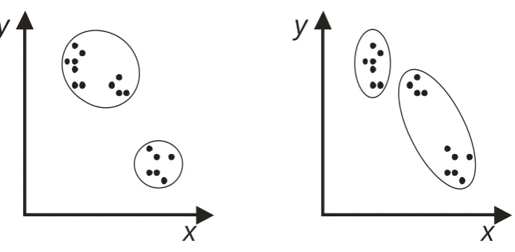
participants preferred to classify the corresponding exemplars along a single

dimension (dimension x in Figure 1a). Observe that along dimension x there is a

well-defined two-cluster category structure, whereas by taking into account dimension y as

well, the resulting category structure is a lot less intuitive. This observation is the

basis of our modeling approach.

---FIGURE 1---

To suggest that unidimensional classification is always preferred is

counterintuitive. First, the literature on basic level categorization shows a preference

for categories maximizing within- and minimizing between-category similarity across

all dimensions (e.g., Gosselin & Schyns, 2001; Rosch & Mervis, 1975). Second, there

are some spontaneous categorization results that do show multidimensional (family

resemblance) classification (e.g., Medin et al., 1987; Milton & Wills, 2004). Finally,

intuitively, when categorizing novel objects in the real world, we do not single out

one dimension, but instead take into account all available useful information. From an

adaptive perspective, a system that indiscriminately ‘ignores’ much of the available

information is likely to miss out on important aspects of its environment.

However, as noted earlier, in experimental settings, the cognitive system does

appear to often ignore much of the available information. Our aim is to explain some

of these conflicting results and intuitions, by providing a model which predicts

preference for unidimensional vs. multidimensional classification, on the basis of the

abstract similarity structure of a set of objects.

Modeling framework

Consider stimuli constructed from two dimensions of physical variation (x, y). Such

or both dimensions equally weighted. For each of these cases, there will be a

classification for the stimuli that is most natural/intuitive, denoted as Group(…).

Group(x), Group(y), Group(x,y), therefore, indicate three classifications, by taking

into account dimension x only, y only, or both, respectively.

The intuitiveness of Group(x) vs. Group(y) vs. Group(x,y) is not necessarily

the same. In Figure 1a, Group(x) is an obvious two-category structure. By contrast,

imagine all the points in Figure 1a collapsed along the y dimension: here we end up

with homogeneous variation along y, there is no obvious category structure. Finally,

Group(x,y) looks a bit like Group(x), but it is not as intuitive since the variation along

the y dimension introduces noise.

Group(x), Group(y), Group(x,y) can therefore vary in intuitiveness. Our

proposal is based on two assumptions: first, the cognitive system can evaluate the

intuitiveness of Group(x), Group(y), Group(x,y) concurrently. Such an assumption is

analogous to computational approaches in perception, whereby it is typically assumed

that several interpretations of a distal layout become available, and can be considered,

concurrently (Pomerantz & Kubovy, 1986). Second, the cognitive system will prefer

unidimensional classification along dimension x (or y) if the intuitiveness of Group(x)

(or Group(y)) is greater than that of Group(x,y). Otherwise, the cognitive system will

prefer a two-dimensional classification. The intuition is that if additional dimensions

do not contribute to (or reduce) the well-formedness of a category structure, then they

are ignored.

To complete the model, what is missing is a measure of category intuitiveness.

There are several candidate models, and an exhaustive examination is simply

categorization: the Rational model (Anderson, 1991), SUSTAIN (Love, Medin, &

Gureckis, 2004), and the simplicity model (Pothos & Chater, 2002).

Rational Model

Anderson’s (1991) Rational model is a Bayesian model of categorization (e.g.,

Tenenbaum, Griffiths, & Kemp, 2006). A new instance, with feature structure F, is

classified to the category k, for which the product P(k)P(F|k) is greatest (or, it may

be assigned to a new category). For example, if you see a new object that looks like a

‘cat’, assign it to the category of cats, since the feature structure of the object is most

probable given this category membership. The term P(F|k)is estimated by taking

into account the expected prior distribution of property values, for each property. For

example, if property values vary continuously,P(F |k)will be calculated on the basis

of a t-distribution, whose parameters depend on the range and mean of the property

values.

The Rational Model is a model of incremental learning. It starts with no

categories; at each step it decides how a novel instance should be categorized, and in

this way eventually builds a classification for a set of stimuli. However, given two

alternative categorizations for the same set of items, it is not possible to decide which

one is psychologically more intuitive. For example, if we consider the Figure 1

stimuli, the Rational Model will very likely produce different classifications

depending on whether the stimuli are represented along x or xy. However, there is no

way to compare the relative goodness of these two classifications and so predict, e.g.,

a preference for unidimensional classification. Moreover, there is a parameter in the

Rational Model (the coupling parameter) which effectively determines how many

categories will be produced for a set of items. As discussed later, this may bias

Overall, the Rational Model cannot be used in the present situation and also,

generally, it is not clear whether it can make predictions with respect to 1d vs. 2d

classification preference. This is not to say that an alternative Bayesian approach may

not provide a compelling account of 1d vs. 2d classification, as Cheng et al.’s (2007)

recent review illustrates.

SUSTAIN

SUSTAIN (Love, Medin, & Gureckis, 2004) is a model that aims to capture the full

continuum between supervised and unsupervised categorization. SUSTAIN is more

powerful than either pure supervised or pure unsupervised categorization models. Its

supervised component is derived from Kruschke’s (1992) ALCOVE model. It

involves attentional parameters which modulate the salience of different dimensions

in the classification of novel instances. SUSTAIN’s unsupervised component is

primarily driven by two principles. First, there is a principle of similarity, favoring

groupings that maximize within-category similarity, while minimizing

between-category similarity. Second, SUSTAIN reacts to ‘surprising’ events. So, for example,

if it encounters a novel instance that does not fit well into any of its existing clusters,

it is likely to create a new cluster. There is a parameter that determines how far a new

instance has to be from existing categories before a new cluster is created; therefore,

this parameter indirectly determines the number of categories. Although Love et al.

(2004) did constrain this parameter to a specific value in their simulations (which was

determined on a priori grounds), its existence somewhat confuses the issue of 1d vs.

2d classification (see the section on Methodological issues).

The attentional parameters of SUSTAIN allow it to model 1d vs. 2d

dissociations. The simulations reported by Love et al. (2004) enable some insight into

that do not inter-correlate with each other, or correlate with each other only partially,

then SUSTAIN tends to produce unsupervised classifications on the basis of a single

dimension—the selected dimension depends on order effects in stimulus presentation

(once SUSTAIN starts to build a clustering, it then adjusts the attentional weights to

favor that clustering, i.e., to make clusters more well-separated). By contrast,

SUSTAIN will produce 2d classifications when the two dimensions are highly

correlated with each other. In cases where there are pairs of correlated dimensions,

higher correlation implies higher probability that SUSTAIN will focus on the

particular pair of dimensions (Gureckis, personal communication). The importance of

dimensional inter-correlation has been highlighted before, for example in the

unsupervised learning study of Billman and Knutson (1996). These investigators

reported results which basically support SUSTAIN’s prediction.

In sum, SUSTAIN can predict unidimensional vs. multidimensional

preference. However, SUSTAIN does not provide a value indicating category

intuitiveness, and so cannot be used in our proposal for 1d vs. 2d classification (for

which it is necessary to compare Group(x) and Group(x,y)).

Simplicity

Rosch and Mervis (1975) suggested that basic level categories maximize within- and

minimize between-category similarity. This intuition can, in principle, allow us to

predict the preferred spontaneous categorization for a set of objects. Pothos and

Chater (2002, 2005) used the simplicity principle to provide a computational

framework for Rosch and Mervis’s suggestion. Simplicity is a principle of

information theory which has been argued to have psychological relevance (Chater,

1999; Feldman, 2000). In its most common form, it states that when there are

categorization, the similarity information between a set of objects can be considered

the ‘data’, which we try to ‘explain’ with different classifications.

The simplicity model first computes the information content of all the

similarity relations between a set of objects. Categories are defined as imposing

constraints on these similarity relations, so that all the objects belonging to a category

are assumed to be more similar to each other, than to any pair of objects belonging to

different categories. Therefore, using categories can reduce the information required

to describe some objects’ similarity structure, if there are numerous and correct such

constraints. Where there are wrong constraints, some information is required to

correct them. Also, specifying an assignment of objects into categories requires some

information. Overall, we can compute the codelength for a set of objects categorized

in a particular way as, {information required before categorization} minus

{constraints minus costs from errors and costs from specifying the category

structure}. The shorter (lower value) the codelength, the more intuitive the

categorization is predicted to be (Figure 2; Appendix). Note that for different sets of

objects the codelength for the best possible classification may be different, depending

on how objects are arranged relative to each other in psychological space (Figure 3).

The simplicity model can compute most intuitive classifications without any

parameters (including number of categories). Therefore, it is suitable for further

specifying our proposal for unidimensional vs. two-dimensional classification.

Finally, as previously noted, SUSTAIN creates new clusters as a reaction to

‘surprising’ events, e.g., encountering new instances that do not fit into the existing

clusters. ‘Surprisingness’ is fundamental to information theory, and therefore the

unsupervised part of SUSTAIN is plausibly similar to the simplicity model.

simplicity approaches can be made equivalent with an appropriate choice of priors

(Chater, 1996). Therefore, implementational differences may obscure intimate

relationships between the three models.

---FIGURES 2,3---

A proposal for 1d vs. 2d classification

Consider again the most intuitive classification along x, y, or by taking into account

both dimensions – Group(x), Group(y), Group(x,y). Using the simplicity model, each

of these classifications can be associated with a codelength value, that determines

how obvious/natural it ought to appear to naïve observers. If Codelength(Group(x)) or

Codelength(Group(y)) are less than Codelength(Group(x,y)), then predict a preference

for unidimensional spontaneous classification (henceforth, Codelength(Group(x)) is

denoted as Codelength(x), etc.) If Codelength(x,y) is less than Codelength(x) and

Codelength(y), then predict a preference for two-dimensional spontaneous

classification. Note that even though the simplicity model has been used in the

formulation of our proposal, it is not necessary: any model that can compute category

intuitiveness without information about the number of categories sought, would have

been equally adequate. As it happens, of the three models of unsupervised

categorization we considered, simplicity was the only one which satisfied these

requirements.

We recognize that a preference for unidimensional vs. two-dimensional

classification may be determined by other biases as well. For example, Regehr and

Brooks (1995) and Milton and Wills (2004; Milton, 2006) highlighted the importance

of procedural details and stimulus format. Medin et al. (1987) observed that a set of

dimension, when there was a way to causally link some of the dimensions (cf.

Wattenmaker et al., 1986, who found that the theme of the stimulus domain could

influence whether a linearly separable classification is favored or not). The

contribution of the present work is that it identifies a way to understand biases on 1d

vs. 2d classification arising from the abstract similarity structure of a set of items. In

some previous studies, such biases have been considered random. For example,

Medin et al. (1987, p.33) state “…there may be no general answer to the question of

which partitioning of some abstract structure of a set of examples is more natural” (a

similar conclusion was reached by Regehr & Brooks, 1995). Thus, the simplicity

approach complements Love et al.’s (2004) effort in this direction, since SUSTAIN

can also predict preference for 1d vs. 2d classification, largely independent of

stimulus format/ procedure. SUSTAIN’s predictions are further discussed after we

report our empirical findings.

Will it be possible to integrate biases on 1d vs. 2d classification from stimulus

format/ procedure, general knowledge, and abstract stimulus structure, into a single,

unifying model? Ideally yes, but currently there are no clues as to how this could be

achieved (cf. Milton & Wills, 2004).

Examining previous findings

The present approach can be readily illustrated with a simplified version of Ashby et

al.’s (1999) data set, shown in Figure 1a. We created a data set of 20 points, 10 points

along each ‘strip’. Both dimensions were assumed to vary from 1 to 10. Similarities

between points were computed using the Euclidean metric. We then used simplicity to

determine Codelength(x) and Codelength(x,y). Codelength values are given in terms

similarity structure with categories, relative to how many bits are required to encode

the same similarity structure without categories. Accordingly, the lower this

percentage value, the smaller the codelength, and so the more intuitive the

corresponding classification is predicted to be (Pothos & Chater, 2002, 2005).

Codelength(x) was 50.07% and Codelength(x,y) was 80.83%. That Group(x) is

predicted to be so much more intuitive compared to Group(x,y) is a straightforward

implication of the fact that along the x dimension there are two extremely

well-separated clusters, whereas, in the xy plane, many between-cluster similarities are

actually greater than within-cluster similarities. Hence, the present formalism readily

predicts that, for the data set in Figure 1a, dimension y will be ignored and

participants should spontaneously classify the items unidimensionally, along

dimension x (consistently with Ashby et al.’s, 1999, findings).

Ashby et al. (1999) also employed data sets as shown in Figure 1b. In such

cases, there was no evidence for a preference either for a two-dimensional

classification (xy) or a unidimensional one (in fact, the two-dimensional classification

could not be learnt without feedback); these researchers found that classifying the

Figure 1a stimuli was a lot easier than classifying the Figure 1b stimuli. The present

model can explain this result. We created a data set to conform to the Figure 1b

category structure. As before, the data set had 20 points, 10 points along each of the

two diagonal strips. Codelength(x,y) was very nearly identical to what we had before

(for Codelength(x,y) for Figure 1a), 81.70%. This is an expected result, since

codelength values are rotationally invariant: the simplicity model does not take into

account the absolute position of points in psychological space, rather it compares

pairs of distances (e.g., it computes whether distance(A,B) is greater than

model, there should be little preference for Group(x,y). Codelength(x) was 81.61%

(compare with the unrotated value: 50.07%) and Codelength(y) was 79.53%.

Therefore, for Figure 1b a classification bias is not predicted for any of Group(x),

Group(y), or Group(x,y), consistently with the results of Ashby et al. (1999).

As noted above, rotation does not alter the 2d codelength, but it can alter the

1d vs. 2d advantage. This is because when the data points are rotated, their 1d

projections change. In Figure 1a there was a well-separated 1d projection, but this is

not the case in Figure 1b. Note that rotating a data set does not imply that the

coordinate axes have to be rotated as well. The alignment of the coordinate axes is

determined by independent, perceptual, considerations (a coordinate axis in

psychological space can be defined as the direction along which only one aspect of a

stimulus’ appearance is altered). Therefore, rotation in 2d can alter the advantage of

the 2d classification relative to the 1d ones, and hence our prediction for

unidimensional vs. two-dimensional classification.

Some of the previous research on 1d vs. 2d classification employed stimuli

composed of discrete, binary features. Each feature would have two possible values,

and each value would correspond to different instantiations of the feature. Although

our model seems to work well with stimuli composed of two continuous dimensions,

it is also useful to consider its predictions with the main stimulus structure employed

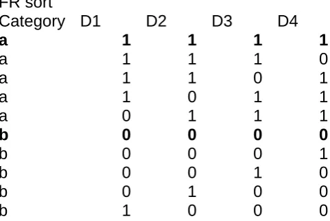
by Medin et al. (1987) and Regehr and Brooks (1995), shown in Figure 4. These

investigators reported a preference for unidimensional classification, across a variety

of procedures and stimulus formats. In order to derive simplicity predictions for the

Figure 4 stimulus structure, we assumed that the 1,0 values are coordinates in a

psychological space, and employed the City block metric to compute similarities. This

effectively corresponds to a count of feature mismatches. Codelength(4d) was

computed to be 94.84%; the optimal classification in 4d was the same as the one

assumed by Medin et al. (1987; shown in Figure 4). By contrast, Codelength(1d) was

only 51.57%. Therefore, our formalism readily explains a preference for

unidimensional classification, as observed by Medin et al. (1987) and Regehr and

Brooks (1995). Note that this prediction relates only to the abstract stimulus structure.

Medin et al. (1987; Experiment 4) employed an alternative data set, whereby

items were created on the basis of four trinary-valued dimensions. In that data set,

Medin et al. claimed that there was no straightforward way to divide the items into

two groups on the basis of one dimension, as requested in their experiments. Ignoring

the requirement to classify the items into two categories (which cannot be modeled

within the simplicity approach), we can still compare Codelength(4d) with

Codelength(1d). We adopted the same approach as before, assuming now that the

values 1, 2, 3 of each trinary dimension correspond to coordinates in a psychological

space (and using the City block metric to compute distances). This approach induces

an ordering in feature values that are nominal: in other words we assume that feature

2 is ‘greater’ than feature 1—clearly this is an approximation. However, it should not

affect the comparison between Codelength(1d) and Codelength (4d) since the same

ordering of feature values is induced in both 1d and 4d. In this case, the former was

61.02% and the latter 56.70%. Therefore, with Medin et al.’s (1987) Experiment 4

data set, a slight preference for 4d classification is predicted. The results of Medin et

al. (1987) were that this category structure prevented 1d classifications, but did not

lead to any 4d ones. Medin et al., however, asked their participants to classify the

stimuli into two groups, a procedure which has been argued to encourage

model predicts a slight preference for 4d classification, with a procedure that

encourages 1d classification, much fewer 1d classifications were observed. We take

this finding to be broadly consistent with the simplicity formalism.

Note that in both the case of Regehr and Brooks (1995) and Medin et al.

(1987) some of the stimuli had limited semantic content. However, it would be

incorrect to perceive the present formalism as applicable in the case of

knowledge-rich stimuli in general. Several investigators have illustrated the complexity of

interactions between general knowledge and spontaneous categorization (e.g., Heit,

1997; Lewandowsky, Roberts, & Yang, 2006; Malt & Sloman, 2007; Wisniewski,

1995), and our formalism would require considerable revision before it can

accommodate general knowledge effects.

In summary, examining previous results on unidimensional vs.

multidimensional classification shows support for the simplicity approach. However,

the experimental and analytical tools employed previously may somewhat bias

spontaneous classification in favor of unidimensional solutions. We discuss these next

and so motivate the need for new experiments using an unconstrained classification

procedure.

---FIGURE 4---

Methodological issues

There are two main methodological issues. First, it is important to ensure that the

experimental procedure does not bias participants to favor, e.g., unidimensional

classifications. Second, it is clearly important to be able to unambiguously infer

In spontaneous classification studies participants are regularly asked to divide

a set of stimuli into two categories. Murphy (2004, p.129) suggested that

college-educated American participants may interpret such a task as a problem-solving one,

whereby they are asked to identify one critical feature that would enable assignment

of the stimuli into two groups. Standardized tests in the US often require searching for

a critical property to distinguish instances and could be the source of such biases in

classification experiments. Therefore, requiring classification into a fixed number of

categories may introduce a response bias for unidimensional classifications,

everything else being equal. Additionally, for a given data set, it is possible that in 2d

there is a very obvious classification into three groups, while in 1d into two groups.

Therefore, asking participants to seek a particular number of clusters may bias them to

take into account both or only one of the available dimensions. To examine

unidimensional vs. two-dimensional classification, an unconstrained categorization

procedure may be preferable.

With respect to the second issue, in unconstrained spontaneous classification

there is considerable response variability. For as few as 10 objects there are about

100,000 possible categorizations (Medin & Ross, 1997). Accordingly, classification

performance has to be measured in terms of preference towards one classification

(e.g., Group(x)) against another (e.g., Group(x,y)). This can be achieved with a

measure of classification similarity, such as the Rand Index (Rand, 1971). The Rand

Index is a statistic that can be utilized in categorization research, to compare two

classifications. It is the ratio of pairs of objects that are both in the same cluster, or

both in different clusters, in the two classifications, divided by all pairs. It varies from

0 (totally different classifications) to 1 (identical classifications). For example,

a unidimensional or two-dimensional bias? Compare Rand(X,Group(x)) with

Rand(X,Group(x,y)). If the second Rand is larger, the participant’s classification is

more similar to the optimal classification in 2d, Group(x,y), and so we can infer that

she had a bias for two-dimensional classification; almost.

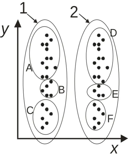
The qualification which needs to be made now relates to the fact that

Group(x,y) and Group(x) are often in a superordinate/ subordinate relationship with

respect to each other. To appreciate the relevance of this point, consider again Figure

1a. A Rand analysis on classification data from Figure 1a could show preference for

Group(x,y) in either of two ways: first, participants indeed consider more intuitive

Group(x,y) and so classify the stimuli by taking into account both dimensions.

Second, participants consider more intuitive Group(x), so they initially classify stimuli

along dimension x, but subsequently seek subclusters along dimension y (Figure 5). In

general, people will often seek to generate classification hierarchies, rather than single

level classifications (e.g., Gosselin & Schyns, 2001). In other words, in Figure 1a,

Group(x,y) is a classification subordinate to Group(x). So, for a stimulus set as shown

in Figure 1a, a Rand Index analysis would be of no use in deciding whether there is a

unidimensional vs. two-dimensional classification bias. Therefore, an appropriate

stimulus design must involve a situation where Group(x)/Group(y) are not subordinate

to Group(x,y) and vice versa. To sum up, when studying the issue of 1d vs. 2d

classification with a spontaneous classification task, the only available empirical

measure is a participant’s classification. Therefore, the classification corresponding to

taking into account a single dimension of variation has to be as different as possible

from the classification taking into account both dimensions of variation. This is why

the stimulus design of Ashby et al. (1999) is not suitable for the present

---FIGURE 5---

A final issue concerns the format of the stimuli. In categorization research,

materials are often created in a way that each stimulus can be perceived as an

individual object, whether this object has some naturalistic appearance (e.g.,

cartoon-like characters or animals, as in Medin et al, 1987) or it corresponds to a meaningless

geometric shape (e.g., lines differing in orientation and length, as in Ashby et al.,

1999). Regehr and Brooks (1995) used stimuli such that each stimulus was a 2d

arrangement of its features separately. For example, a stimulus could be composed of

a bottle, a cup, a trumpet, and a cake, enclosed within a rectangle. Milton and Wills

(2004; Milton, 2006; Handel & Imai, 1972) observed that stimulus format does affect

unidimensional vs. multidimensional classification, but it was difficult to formulate

general principles.

The simplicity approach can only explain biases arising from the abstract

stimulus structure, not stimulus format or other procedural details. Therefore, we

simply chose two-dimensional stimuli that could be perceived as individual objects, as

is most commonly done in categorization research. Also, we aimed for dimensions of

physical variation that would be neither particularly separable nor integral, since this

could potentially influence unidimensional preference (Milton, 2006). Crucially, with

the Rand Index analysis, it is not necessary to ensure that the stimulus dimensions do

not introduce a bias for unidimensional vs. multidimensional preference. Suppose that

the stimulus format encourages multidimensional classification. The Rand Index

should still reveal a bias for unidimensional classification where one is predicted,

relative to the condition where multidimensional classification is predicted. That is,

there should be more of a bias for Group(x) when we predict that Group(x) ought to

Experimental investigation

Design

Forty Cardiff University students took part for course credit. Twenty participants were

allocated to a condition where a preference for unidimensional classifications was

predicted, and 20 to a condition where a preference for two-dimensional

classifications was predicted. An additional 24 paid participants were recruited from

the Cardiff University student population to provide similarity ratings.

Materials

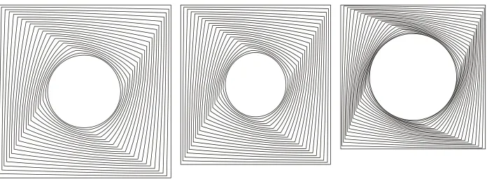
Stimuli were circles enclosed in squares, with the circles ‘blended in’ with the squares

(using CorelDraw), so as to make them look more like individual objects (Figure 6).

The similarity structure for the two conditions (to be discussed shortly) was specified

on abstract 1-10 scales; therefore, these scales had to be mapped to the physical

dimensions of circle size and square size. This was done by assuming a Weber’s

fraction of 7.5% for both the circles (smallest size 25mm) and the squares (smallest

size: 50mm; Morgan, 2005). Each stimulus was printed individually on a piece of

paper as large as the stimulus, which was subsequently laminated.

---FIGURE 6---

As noted, our objective was to create a stimulus structure such that

Group(x)/Group(y) were not superordinate or subordinate relative to Group(x,y).

Figure 7 shows such a stimulus structure, for which we predict unidimensional

classification, since Codelength(x), Codelength(y) are less than Codelength(x,y).

Notice that in two dimensions there are two barely distinguished clusters, whereas

along either x or y there are three, reasonably well-separated groups (Group(x),

classifications). By contrast, for the items in Figure 8 we predict that participants will

favor Group(x,y) over either Group(x) or Group(y): in two dimensions there are three

fairly obvious groups, whereas along either of dimensions x or y there is basically a

uniform distribution of items. The stimulus sets were created so that the codelengths

for the optimal classifications in each condition are approximately the same, and

likewise for the suboptimal ones (of course, in one condition the optimal classification

is two-dimensional, in the other unidimensional).

---FIGURES 7,8---

In sum, we have a stimulus set for which unidimensional spontaneous

classification is predicted and one for which two-dimensional classification is

predicted, so that the Group(x)/Group(y) classifications in each case are not

superordinate or subordinate to the Group(x,y) one.

Participants may spontaneously classify the stimuli in terms of both or only

one of the dimensions, but, either way, it is important to establish that they perceived

the stimuli as we intended them to. We collected similarity ratings from12

participants for each of our two stimulus sets separately. Participants were instructed

that their task was to rate the similarity between a number of different items. The 20

stimuli in either of the two data sets were then sequentially displayed on a computer

screen in a random order. Stimuli were displayed for 1000 ms each, and each item

was preceded by a centrally located fixation point, displayed for 250ms.

Subsequently, participants were instructed that they would have to rate the similarity

between the stimuli on a scale ranging from 1 (very dissimilar) to 9 (very similar).

Each trial consisted of a central fixation point (250ms), followed by the first stimulus

(1000ms), followed by another fixation point (250ms) and the second stimulus

Participants rated the similarity of all possible stimulus pairs once, excluding pairs of

identical stimuli, for a total of 380 similarity comparisons. Trials were randomly

ordered.

We used the Multidimensional Scaling (MDS) procedure to derive a spatial

representation in 2d for the stimuli, on the basis of their similarity ratings. For the data

set for which a 1d classification was predicted, the best solution was associated with a

stress of 0.168 (lower values indicate better solution), and for the data set for which a

2d classification was predicted stress was 0.149.

The Orthosim procedure (Barrett et al., 1998) allows the computation of

various similarity indices between two sets of coordinates for the same set of items. In

our case, we wished to compare the similarity of the MDS-derived representation for

the stimuli with the experimenter-assumed coordinates (on the basis of which the

predictions for unidimensional vs. multidimensional classification were computed).

We selected a similarity index which adopts a ‘procrustes’ approach (Barrett et al.,

1998), according to which the coordinate configurations to be compared are first

normalized and rotated/ reflected to remove any of the arbitrariness in MDS solutions

(with respect to location, scale, and orientation). The Orthosim documentation

recommends the ‘double-scaled Euclidean distance’ coefficient, for which 0

corresponds to complete dissimilarity, 1 to identity. The similarity coefficient between

the coordinates for the data set for which 1d classification was predicted and the

corresponding MDS solution was 0.74 and for the data set for which 2d classification

was predicted 0.72. In evaluating these results, note that the similarity ratings

procedure leads to very noisy data, for a number of reasons: a similarity scale is a

rather insensitive measure of similarity perception and the ratings task is so long that

procedures, such as confusability ratings, are not appropriate in our case, since our

stimuli are highly discriminable relative to each other. Overall, we consider the

similarity between the experimenter assumed coordinates and the corresponding MDS

solutions adequate.

A final issue that needs to be addressed is whether our predictions might be

valid after some radical restructuring of the similarity space, as a result of processing

the stimuli. For example, what if participants gradually represented the stimuli

corresponding to Figure 8 on the basis of a single, composite, emergent dimension

along the diagonal? Such a possibility seems very unlikely. First, we are not aware of

any process of perceptual learning which posits the emergence of such composite

dimensions of variation. Second, such radical restructuring of the similarity space

would require extensive learning, rather than casual processing of the stimuli, as was

the case in our experiments (e.g., Goldstone, 1994, 2000).

Procedure

Participants were presented with one of the two stimulus sets and asked to categorize

the items in a ‘natural and intuitive way’. They were told that they could use as many

groups as they wanted, but no more than they felt necessary. Participants received the

stimuli in a randomly ordered stack and subsequently spread them out on a table to

determine the preferred classification, by arranging the stimuli into piles. Participants

were free to compare the stimuli in any way they wished, and to make alterations to

any initial groups they formed.

Results

Our objective was to examine when participants were more likely to generate

classifications similar to Group(x)/Group(y) vs. Group(x,y). As mentioned before,

frequency of occurrence of different classifications (Medin & Ross, 1997); therefore,

the Rand Index was employed.

Each participant generated a classification. If a participant was biased to prefer

e.g. Group(x) over and above Group(x,y), then we would expect the Rand similarity

between the participant’s classification and Group(x) to be higher than between the

participant’s classification and Group(x,y). Accordingly, for all participants in each

condition separately, we computed the Rand similarity of the classifications they

produced with Group(x), Group(y), and Group(x,y) (for each condition the optimal

classifications are different). Note that participants might prefer Group(x) over

Group(y) if the squares dimension is more salient than the circles one. We are not

interested in such differences, but rather in when either Group(x) or Group(y) is

preferred over Group(x,y). Accordingly, we infer unidimensional preference if Rand

similarity to Group(x) or Group(y) is greater than to Group(x,y), and two-dimensional

preference otherwise.

The dependent variable was the similarity of participants’ classifications to

Group(x), Group(y), and Group(x,y), as computed by the Rand Index. One two-way

ANOVA was run with ‘condition’ as a between-participants factor and ‘similarity to

Group(x) vs. Group(x,y)’ as a within-participants factor. A second two-way ANOVA

was run with ‘condition’ as a between-participants factor again and ‘similarity to

Group(y) vs. Group(x,y)’ as the within-participants factor. In both cases the

interaction between the two factors was significant (Figure 9; F(1,38) = 326.819,

p<.0005 and F(1,38) = 48.290, p<.0005, respectively). In the case where we predicted

unidimensional classification, the similarity of participants’ classifications to

Group(x,y) was less than to both the similarity to Group(x) and similarity to Group(y),

and t(19) = -2.951, p=.004, respectively). In the case where we predicted

two-dimensional classification, similarity to Group(x,y) was greater than both the

similarity to Group(x) and similarity to Group(y), assessed in the same way (t(19) =

21.731, p<.0005, and t(19) = 6.441, p<.0005, respectively).

---FIGURE 9---

Other models

SUSTAIN spontaneously classifies a set of stimuli on the basis of more than one

dimensions when (and for) dimensions which are highly intercorrelated with each

other. Therefore, we can examine the correlations between the dimensions in the two

datasets we employed. For the data set for which 1d classification was predicted, the

correlation between the two dimensions was .763 (p < .01) and for the data set for

which 2d classification was predicted, the correlation was nearly identical, .760 (p <

.01). However, in one case we predicted 1d classification and in the other 2d

classification. Therefore, the simplicity model specifies a bias for 1d vs. 2d

classification that is separate from the one derived from SUSTAIN. Note, however,

that this may be an unfair comparison: SUSTAIN is a model of incremental learning,

whereas the simplicity approach was specifically designed to be applicable in

situations when all the stimuli appear simultaneously (cf. simplicity models of

perceptual organization; e.g., Pomerantz & Kubovy, 1986). Note also that the

simplicity approach predicts that classification intuitiveness remains unchanged by

adding dimensions perfectly correlated with existing ones (recall, that the simplicity

model does not encode absolute point locations, rather pairs of similarities). However,

methodologically it is very difficult to examine whether spontaneous categorization

subsumes the two correlated dimensions). Billman and Knutson (1996) reported that

correlated dimensions facilitate the learning of a target rule, but the link between

spontaneous generation of categories and unsupervised learning is not straightforward

(cf. Murphy, 2004).

Models of supervised categorization that employ free parameters for

attentional weighting can, of course, describe the reported results. However, without

some constraints on determining these parameters a priori, it is unclear as to how such

models can predict our results (e.g., Nosofsky, 1989). Additionally, there are other

approaches of unsupervised categorization which we did not consider at all (e.g.,

Compton and Logan, 1993; Schyns, 1991). The emphasis on SUSTAIN and the

Rational Model has been guided by a number of considerations (similar points apply

to the simplicity model). First, several researchers have recently made compelling

arguments for the relevance of simplicity and Bayesian principles in modeling human

cognition (e.g., Chater, 1999; Feldman, 2000; Tenenbaum et al., 2006). The Rational

Model was specifically developed as a Bayesian model of category learning; an

important component of SUSTAIN’s operation is a principle of surprisingness, which

can be interpreted in simplicity terms. Second, both models are flexible enough to

allow predictions across a variety of modeling situations, without modification (e.g.,

regardless of whether stimuli are represented in terms of features or continuous

dimensions of variation). It would be undesirable to consider models that could not (in

principle) be applied to the range of results examined in this work. Third, they have a

limited number of reasonably well-constrained parameters. In fact, in both cases

model parameters are often treated as fixed (the coupling parameter in the Rational

parameters for each of their demonstrations separately). Finally, SUSTAIN has

specifically been applied to the problem of 1d vs. 2d classification.

Finally, can our results be captured by a statistical clustering algorithm (for a

review with an emphasis on psychological categorization see Pothos and Chater,

2002; more generally, see, Fisher & Langley, 1990 or Krzanowski & Marriott, 1995)?

Note that a statistical algorithm must have some psychological interpretation before it

can be considered as a candidate explanation for human categorization. Certain

versions of K-means clustering are a possibility, since they can identify clusters

maximizing within cluster similarity while minimizing between cluster similarity.

However, they require information about the number of categories sought (K). As

noted above, such information may prejudice the issue of whether a unidimensional or

multidimensional classification is optimal.

Discussion

When participants are asked to spontaneously categorize a set of objects, will they

take into account only one of the objects’ dimensions or all of them? Most empirical

results argue in favor of a unidimensional preference (Ashby et al., 1999; Medin et al.,

1987; Regehr & Brooks, 1995). A preference for multidimensional classification has

been observed, by manipulating the stimulus format and experimental procedure (e.g.,

Handel & Imai, 1972; Milton, 2006), or by providing a causal scenario to relate the

dimensions of a set of objects (Medin et al., 1987). To our knowledge, ours is the first

empirical demonstration showing a two-dimensional bias in spontaneous

classification, on the basis of the abstract stimulus structure. We were able to predict

unidimensional vs. two-dimensional preference, by employing Pothos and Chater’s

unidimensional classification when the (optimal) classification along any single

dimension is more intuitive than the classification taking into account both

dimensions, and vice versa. Our results support the simplicity approach, and illustrate

that the stimuli/ procedure we employed could not have had a confounding influence,

since with stimuli of exactly the same format we could predict both unidimensional

and two-dimensional classification.

The empirical test of our hypothesis involved two methodological innovations.

First, we used the Rand Index of classification similarity, which allowed us to employ

an unconstrained categorization procedure. As Murphy (2004) argued, requiring

participants to divide the items into a fixed number of dimensions may favor

unidimensional classification. Second, we recognized that data sets as in Figure 1a

make it difficult to establish unambiguously unidimensional vs. two-dimensional

classification, since (in this case) the former is superordinate to the latter (Figure 5).

Thus, stimulus structures had to be specified where the optimal unidimensional

classification was not related to the optimal two-dimensional classification in a

superordinate/subordinate way (Figures 7, 8).

Research into unidimensional vs. multidimensional classification may shed

light on Goodman’s paradox. Goodman (1972; see also Goldstone, 1994; Pothos,

2005; Sloman & Rips, 1998) observed that any two items may be understood as

arbitrarily similar, depending on which of their properties are considered. For

example, a giraffe and a house can both be very similar if one considers the fact that

they both weigh less than 10 tons, less then 11 tons etc. (cf. Barsalou, 1991). Of

course, when considering such properties, our natural intuition is that they are

nonsense and ought to be ignored. Strong as this intuition is, it has been difficult to

perceived only with the dimensions that lead to the most intuitive classification for the

stimuli (cf. Kruschke, 2006; Nosofsky, 1989). In other words, the flexibility of

similarity could be constrained by observing which subset of possible object

dimensions lead to well-formed categories. Note, however, that understanding

similarity/representation has proved an immensely complicated problem in

psychology (Griffiths, Steyvers, & Tenenbaum, 2007), and the above idea is likely to

provide only a partial solution. For example, there is ample evidence that similarity

judgments can be also be constrained by considering general knowledge influences

Acknowledgements

This research was partly supported by ESRC grant R000222655 and EC Framework 6

grant contract 516542 (NEST). We would like to thank Lee Brooks, Nick Chater,

Ulrike Hahn, Peter Hines, Matt Jones, Amotz Perlman, an anonymous reviewer, and

particularly Todd Gureckis for their useful comments. We are also grateful to Paul

Barrett for his help with the Orthosim software, which can be obtained from his

website: http://www.pbarrett.net/.

References

Ahn, W. & Medin, D. L. (1992). A two-stage model of category construction.

Cognitive Science, 16, 81-121.

Anderson, J. R. (1991). The Adaptive Nature of Human Categorization. Psychological

Review, 98, 409-429.

Ashby, F. G., Queller, S., & Berretty, P. M. (1999). On the dominance of

unidimensional rules in unsupervised categorization. Perception & Psychophysics,

61, 1178-1199.

Barrett, P. T., Petrides, K. V., Eysenck, S. B. G., & Eysenck, H. J. (1998) The

Eysenck Personality Questionnaire: An examination of the factorial similarity of P,

E, N, and L across 34 countries. Personality and Individual Differences, 25, 5,

805-819.

Barsalou, L. W. (1991). Deriving categories to achieve goals. In G. H. Bower (Ed.),

The psychology of learning and motivation, Vol. 27, pp. 1-64. New York:

Billman, D. & Knutson, J. (1996). Unsupervised concept learning and value

systematicity: A complex whole aids learning the parts. Journal of Experimental

Psychology: Learning, Memory, and Cognition, 22, 458-475.

Chater, N. (1996). Reconciling Simplicity and Likelihood Principles in Perceptual

Organization. Psychological Review, 103, 566-591.

Chater, N. (1999). The Search for Simplicity: A Fundamental Cognitive Principle?

Quarterly Journal of Experimental Psychology, 52A, 273-302.

Cheng, K., Shettleworth, S. J., Huttenlocher, J., & Rieser, J. J. (2007). Bayesian

integration of spatial information. Psychological Bulletin, 133, 625-637.

Compton, B. J. & Logan, G. D. (1993). Evaluating a computational model of

perceptual grouping. Perception & Psychophysics, 53, 403-421.

Feldman, J. (2000). Minimization of Boolean complexity in human concept learning.

Nature, 407, 630-633.

Fisher, D., & Langley, P. (1990). The structure and formation of natural categories. In

Gordon Bower (Ed.), The Psychology of Learning and Motivation, Vol. 26 (pp.

241-284). San Diego, CA: Academic Press.

Goldstone, R. L. (1994). The role of similarity in categorization: providing a

groundwork. Cognition, 52, 125-157.

Goldstone, R. L. (2000). Unitization during category learning. Journal of

Experimental Psychology: Human Perception and Performance, 26, 86-112.

Goodman, N. (1972). Seven strictures on similarity. In N. Goodman, Problems and

projects (pp. 437-447). Indianapolis: Bobbs-Merrill.

Gosselin, F. & Schyns, P. G. (2001). Why do we SLIP to the basic-level?

Computational constraints and their implementation. Psychological Review, 108,

Griffiths, T. L., Steyvers, M., & Tenenbaum, J. B. (2007). Topics in semantic

representation. Psychological Review, 114, 211-244.

Hampton, J. A. (2003). Abstraction and context in concept representation.

Philosophical Transactions of the Royal Society of London B, 358, 1251-1259.

Handel, S. & Imai, S. (1972). The Free Classification of Analyzable and

Unanalyzable Stimuli. Perception & Psychophysics, 12, 108-116.

Heit, E. (1997). Knowledge and Concept Learning. In K. Lamberts & D. Shanks

(Eds.), Knowledge, Concepts, and Categories (pp. 7-41). London: Psychology

Press.

Krzanowski, W. J. & Marriott, F. H. C. (1995). Multivariate Analysis, Part 2:

Classification, Covariance Structures and Repeated Measurements. Arnold: London.

Kruschke, J. K. (2006). Locally Bayesian learning with applications to retrospective

reevaluation and highlighting. Psychological Review, 113, 677-699.

Kruschke, J. K. (1993). Human category learning: Implications for backpropagation

models. Connection Science, 5, 3-36.

Kruschke, J. K. (1992) ACLOVE: An exemplar-based connectionist model of

category learning. Psychological Review, 99, 22-44.

Lewandowsky, S., Roberts, L., & Yang, L. (2006). Knowledge partitioning in

categorization: boundary conditions. Memory & Cognition, 34, 1676-1688.

Love, B. C., Medin, D. L., & Gureckis, T. M. (2004). SUSTAIN: A network model of

category learning. Psychological Review, 111, 309-332.

Malt, B. C. & Sloman, S. A. (2007). Category essence or essentially pragmatic?

Creator’s intention in naming and what’s really what. Cognition, 105, 615-648.

Medin, D. L. & Ross, B. H. (1997). Cognitive psychology. (2nd Ed.). Fort Worth:

Medin, D. L., Wattenmaker, W. D., & Hampson, S. E. (1987). Family resemblance,

conceptual cohesiveness, and category construction. Cognitive Psychology, 19,

242-279.

Milton, F. (2006). Category construction: A study of the principles underlying

category formation. Unpublished PhD thesis, University of Exeter.

Milton, F. & Wills, A. J. (2004). The influence of stimulus properties on category

construction. Journal of Experimental Psychology: Learning, Memory, and

Cognition, 30, 407-415.

Morgan, M. J. (2005). The visual computation of 2-D area by human observers.

Vision Research, 45, 2564-2570.

Murphy, G. L. (2004). The big book of concepts. MIT Press: Cambridge, USA.

Nosofsky, R. M. (1989). Further tests of an exemplar-similarity approach to relating

identification and categorization. Journal of Experimental Psychology: Perception

and Psychophysics, 45, 279-290.

Nosofsky, R. M., Palmeri, T. J., & McKinley, S. C. (1994). Rule-plus-exception

model of classification learning. Psychological Review, 101, 53-79.

Pomerantz, J. R. & Kubovy, M. (1986). Theoretical Approaches to Perceptual

Organization: Simplicity and Likelihood principles. In: K. R. Boff, L. Kaufman & J.

P. Thomas (Eds.), Handbook of Perception and Human Performance, Volume II:

Cognitive Processes and Performance, 1-45. New York: Wiley.

Pothos, E. M. (2005). The rules versus similarity distinction. Behavioral & Brain

Sciences, 28, 1-49.

Pothos, E. M. & Chater, N. (2002). A Simplicity Principle in Unsupervised Human

Pothos, E. M. & Chater, N. (2005). Unsupervised categorization and category

learning. Quarterly Journal of Experimental Psychology, 58A, 733-752.

Rand, W. M. (1971). Objective Criteria for the evaluation of clustering methods.

Journal of the American Statistical Association, 66, 846-850.

Regehr, G. & Brooks, L. R. (1995). Category organization in free classification: The

organizing effect of an array of stimuli. Journal of Experimental Psychology:

Learning, Memory, and Cognition, 21, 347-363.

Rissanen, J. (1989). Stochastic complexity and statistical inquiry. Singapore: World

Scientific.

Rosch, E. & Mervis, B. C. (1975). Family Resemblances: Studies in the Internal

Structure of Categories. Cognitive Psychology, 7, 573-605.

Schyns, P. G. (1991). A Modular Neural Network Model of Concept Acquisition.

Cognitive Science, 15, 461-508.

Sloman, S. A. & Rips, L. J. (1998). Similarity as an explanatory construct. Cognition,

65, 87-101.

Sloman, S. A., Love, B. C., & Ahn, W. (1998). Feature Centrality and Conceptual

Coherence. Cognitive Science, 22, 189-228.

Tenenbaum, J. B., Griffiths, T. L., & Kemp, C. (2006). Theory-based Bayesian

models of inductive learning and reasoning. Trends in Cognitive Sciences, 10,

309-318.

Wattenmaker, W. D., Dewey, G. L., Murphy, T. D., Medin, D. L. (1986). Linear

Separability and Concept Learning: Context, Relational Properties, and Concept

Wisniewski, E. J. (1995). Prior knowledge and functionally relevant features in

concept learning. Journal of Experimental Psychology: Learning, Memory, and

Appendix

Computations for the simplicity model involve three steps.

First, we compute the information-theoretic codelength required to describe the

similarity structure of a set of objects, without any categories. This is done by

considering all pairs of similarities. For example, for four objects A, B, C, and D, we

are interested in whether

sim(A,B) >< sim(A,D)

sim(A,B) >< sim(A,C)

sim(A,B) >< sim(B,D)

sim(A,B) >< sim(B,C)

etc.

Note that determining each of these inequalities is worth one bit of information, since

there are only two possibilities (equalities are ignored; in real life this is not a

problem, in practice the formalism is slightly adjusted to take into account equalities).

For example, for 10 objects, there are 10*(10-1)/2 = 45 similarities (assuming

symmetry and minimality), hence there are 990 pairs of similarities. Thus, to describe

the similarity structure of 10 objects, a codelength of 990 bits is required.

Second, categories impose constraints on the similarity structure of the items.

Specifically, define categories as implying that all within category similarities are

greater than all between category similarities. For example, suppose that 10 objects

can be divided into two perfect categories (that is, no constraints are violated). Then,

In both categories together we have 20 within category similarities. Also, we have

5*5 between category similarities. Therefore, in total, there are 20*25=500

constraints. So, with categories, to describe the similarity structure of the items almost

(see below) 990-500=490 bits are required. In Pothos and Chater’s (2002) model it is

this information-theoretic simplification that makes categorization useful.

Third, we need to encode the particular classification that is utilized. This is done

using Stirling’s number, (1)v (nv)

r

(nv)!v!

v0

n



which r items can be divided into n categories. The increase in codelength due to this

term is typically small. Also, in general some of the constraints imposed by a

classification will be wrong, and we have to correct them. If we have u constraints

and e errors, then we require log₂(u1)log₂

 

u!

e!(ue)!.

Overall, the codelength for the similarity structure for a set of objects is reduced by

the constraints of the classification, but increased by having to correct for errors and

to specify the classification. The lower the overall codelength, the more intuitive the

classification is predicted to be, in accord with the algorithmic simplicity framework

of Minimum Description Length (Risannen, 1989).

Figures:

Figure 1. Two of the data sets employed by Ashby at al. (1999). (The data sets are not

identical to the ones used by Ashby et al.) Here and elsewhere the dimensions x and y

are assumed to correspond to dimensions of physical variation. For the ‘a’ data set,

participants preferred to classify the items along the single dimension x (the

perforated line shows the preferred classification), rather than produce classifications

compatible with both dimensions x, y. For the ‘b’ data set, none of the participants

responded optimally.

a

x

y

b

x

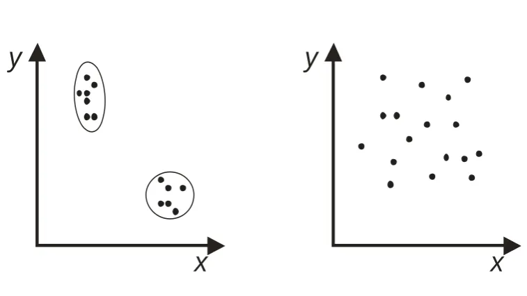
Figure 2. The simplicity model can evaluate the relative intuitiveness of different

classifications for the same set of objects. In this case, the classification on the left is

predicted as more intuitive (and will be associated with a smaller codelength), as it

involves better-separated clusters.

x

y

Figure 3. For the objects in the left-hand panel, the best possible classification is

associated with a smaller codelength, than the best possible classification for the

objects in the right-hand panel (for which there are very weak intuitions about any

classification). Such differences reflect the intuition that different sets of objects could

be classified in a more or less obvious way.

x

y

Figure 4. The abstract stimulus structure employed by Medin et al. (1987) and Regehr

and Brooks (1995). The first column indicates the assumed optimal classification of

the items, if all four dimensions are taken into account (this is the FR, or family

resemblance, classification). In boldface are shown the assumed prototypes of each

category (in 4d).

FR sort

Category D1 D2 D3 D4

a 1 1 1 1

a 1 1 1 0

a 1 1 0 1

a 1 0 1 1

a 0 1 1 1

b 0 0 0 0

b 0 0 0 1

b 0 0 1 0

b 0 1 0 0

Figure 5. Participants might either classify the stimuli two-dimensionally, producing

clusters A, B, C, D, E, F, or they might first classify the stimuli unidimensionally

along x (as we would expect), producing clusters 1, 2, and then subsequently look for

subclusters within 1 and 2, so that the end classification would also be A, B, C, D, E,

F. Thus, a stimulus set like that of Figure 1a is unsuitable for studying unidimensional

vs. two-dimensional classification.

x

y

A

B

C

D

E

F

Figure 6. A few examples of the stimuli employed in the present study. The stimulus on the left shows the greatest size in the square dimension,

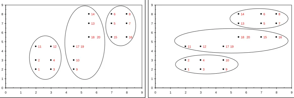
Figure 7. A stimulus structure where the simplicity approach predicts that participants

will prefer a unidimensional classification (the 1d classifications are shown). Where

there are two numbers next to a point, this means that two identical items were

included in the stimulus set. The most intuitive classification along x is (1,2,3,4,11,12)

(5,6,7,8,15,16) (9,10,13,14,17,18,19,20) and along y (1,2,3,4,9,10) (5,6,7,8,13,14)

(11,12,15,16,17,18,19,20), both with a codelength of 57.6%, and the most intuitive

classification along xy is (1,2,3,4,9,10,11,12) (5,6,7,8,13,14,15,16,17,18,19,20) with a

codelength of 73.4%.

18 17 16 15 14 13 12 11 10 9 8 7 6 5 4 3 2 1 0 1 2 3 4 5 6 7 8 9

0 1 2 3 4 5 6 7 8 9

19 20 18 17 16 15 14 13 12 11 10 9 8 7 6 5 4 3 2 1 0 1 2 3 4 5 6 7 8 9

0 1 2 3 4 5 6 7 8 9

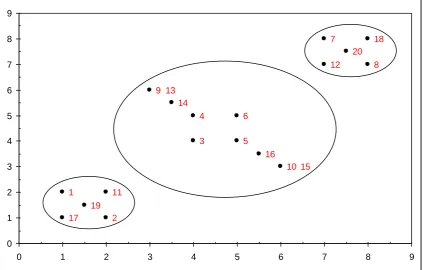
Figure 8. A stimulus structure where the simplicity approach predicts that participants

will prefer the two-dimensional classification (the 2d classification is shown). The

most intuitive classification along x is (1,2,3,4,9,11,13,14,17,19)

(5,6,7,8,10,12,15,16,18,20) and along y (1,2,3,5,10,11,15,16,17,19)

(4,6,7,8,9,12,13,14,18,20), both with a codelength of 73.5%, and the most intuitive

classification along xy is (1,2,11,17,19) (3,4,5,6,9,10,13,14,15,16) (7,8,12,18,20) with

a codelength of 59.4%.

20 19 18 17 16 14 12 11 10 9 8 7 6 5 4 3 2 1 0 1 2 3 4 5 6 7 8 9

0 1 2 3 4 5 6 7 8 9

Figure 9. The Rand Index analyses results. ‘Rand to x’ means Rand similarity of

participants’ classifications to Group(x) etc. ‘Unidimensional Preference’ refers to the

condition where simplicity predicts a preference for unidimensional classification.

‘Two-dimensional Preference’ refers to the condition where simplicity predicts a

preference for two-dimensional classification. Error bars denote one standard

deviation.

0.81

0.68

0.63

0.65 _0.64

0.79

0.00 0.10 0.20 0.30 0.40 0.50 0.60 0.70 0.80 0.90 1.00

Rand to x Rand to y Rand to xy