City, University of London Institutional Repository
Citation
:
Reyes-Aldasoro, C. C. (2009). Retrospective shading correction algorithm based on signal envelope estimation. Electronics Letters, 45(9), pp. 454-456. doi: 10.1049/el.2009.0320This is the unspecified version of the paper.
This version of the publication may differ from the final published
version.
Permanent repository link:
http://openaccess.city.ac.uk/3741/Link to published version
:
http://dx.doi.org/10.1049/el.2009.0320Copyright and reuse:
City Research Online aims to make research
outputs of City, University of London available to a wider audience.
Copyright and Moral Rights remain with the author(s) and/or copyright
holders. URLs from City Research Online may be freely distributed and
linked to.
A retrospective shading correction algorithm based on
signal envelope estimation
Constantino Carlos Reyes-Aldasoro
Cancer Research UK Tumour Microcirculation Group, Academic Unit of
Surgical Oncology. The University of Sheffield, K Floor, School of Medicine &
Biomedical Sciences, Beech Hill Road, Sheffield S10 2RX, U.K.
Abstract
An additive retrospective non-parametric algorithm for the correction of
inhomogeneous intensity background of images, commonly known as
shading, is presented. The algorithm assumed that an original unbiased
image was corrupted by a slowly-varying shading that could be estimated
from the signal envelope in a process analogous to amplitude modulation
detection. Unlike other filtering algorithms, the algorithm did not require
pre-processing, parameter setting, user interaction, computationally intensive
optimisation algorithms nor a restriction in size of the objects of interest
relative to the scale of background variations. The algorithm provided
satisfactory results for artificial and microscopical images.
Introduction
A common phenomenon in biomedical imaging is the presence of spurious
intensity variations due to the sample of interest and the technique of
acquisition. In light microscopy, the variation may originate from uneven
Köhler illumination and is commonly known as shading [1-4]. In magnetic
resonance imaging, intensity inhomogeneity or bias field may be caused by
variation in the radio-frequency (RF) coil uniformity, static field inhomogeneity,
RF penetration, as well as the anatomy and position of the sample [5-7].
Correction methods can be prospective when a calibration protocol and extra
images are acquired, or retrospective when the only data available is the
image itself. When shading is caused by the object, it can only be removed by
a retrospective algorithm [8].
The first class of correction algorithms apply filtering with low pass,
homomorphic or morphological operators as it is a simple and intuitive way of
removing low frequency shading components [3]. However, a limitation of
these methods is that they assume that the background is either darker or
brighter than the objects of interest, and that these are limited in size and
smaller than the background variations. In [8] several methods were
compared and all filtering methods failed to correct images with large objects.
A second class of algorithms use surface fitting methods [3, 9] require the
selection of a number of points on the background, either manually or
automatically, and the background is obtained by the fitting of a parametric
surface. Manual selection is subjective and time consuming and automated
methods assume a good global support of the background, which is not
always the case. These methods also failed to correct images with large
objects. A third class of algorithms perform entropy minimisation [4, 10] as it is
assumed that the shading introduces extra information to the image, which
manifests itself as a higher entropy. A parametric polynomial surface that
performed well with all types of images, with either large or small objects. A
disadvantage of this method is that an accurate approximation of certain
surfaces (one with a small local variation, for example) may require a high
order polynomial, and consequently a computationally expensive optimisation
process. In practice, the polynomials are restricted to be of lower orders: first
or second.
This letter presents an algorithm to remove the shading component of images
by estimating the envelope of the signal. The process of estimation could be
understood as the iterative stretching of a thin flexible surface under which (or
over which) a series of objects are placed. Initially, the surface was identical
to the signal intensity but after a series of stretches, the surface adapted to
the peaks (or lowest points) of the objects, and intermediate values in
between them. The algorithm made no assumptions regarding whether the
objects were of higher or lower intensity than the background and performed
well with small and large objects as well as different microscopical images.
Algorithm
The acquired, shaded image I(x,y) was assumed to be formed by an additive
shading component S(x,y) which corrupted an original unbiased image U(x,y)
I(x,y) = U(x,y) + S(x,y) (1)
Therefore, the corrected image Û(x,y), which was an estimation of U(x,y), was
given by:
The shading correction algorithm estimated the slowly-varying shading
component or inhomogeneous background from the envelope of the
rapidly-varying signal in a way analogous to the well-known amplitude modulation
(AM) detection where a slowly varying function or modulating signal alters the
amplitude (or intensity) of a rapidly varying signal or carrier [11]. First, the
signal was low-pass filtered with a 3×3 Gaussian kernel to minimise the
effects of noise. Then, to obtain the envelope, the algorithm scanned every
pixel of the image and compared its intensity with the average value of
increasingly distant pairs of opposite 8-connectivity neighbours in 4
orientations: [0°, 45°, 90°, 135°]. Two series of new surfaces Smax/Smin were
generated by replacing the intensity of the pixel by the maximum/minimum
value of the comparison at every distance di for each iteration i. To obtain the
upper envelopeSmax, the intensity of the pixel was replaced with the maximum
value of the averages and the pixel itself:
Si
max(x,y)=max
I(x−di,y−di)+I(x+di,y+di)
2 ,
I(x+di,y−di)+I(x−di,y+di)
2 ,
I(x−di,y)+I(x+di,y)
2 ,
I(x,y−di)+I(x,y+di)
2 ,I(x,y)
⎧ ⎨ ⎪⎪ ⎩ ⎪ ⎪ ⎫ ⎬ ⎪⎪ ⎭ ⎪ ⎪ (3).
For the lower envelope, the replacement corresponded to the minimum value.
The maximum/minimum values of the series of surfaces formed two stacks
from which the maximum intensity projection corresponded to the current
envelope estimation: Simax(x,y)=max
i S
i
max(x,y)
{
}
. Both surfaces Simax/S
i
min were
to spread the envelope estimation to those pixels with intermediate
orientations. The process was repeated by increasing di and the size of the
filter, thus allowing the envelope to adapt to objects of different sizes. To
determine a stop criterion, local derivatives
∂Si
max/min
∂x ,
∂Si
max/min
∂y , (4)
and the magnitude of the gradient (MGi) were calculated:
MGi = ∂S i max/min ∂x ⎛ ⎝⎜ ⎞ ⎠⎟ 2
+ ∂Simax/min ∂y ⎛ ⎝⎜ ⎞ ⎠⎟ 2 ⎛ ⎝ ⎜ ⎞ ⎠ ⎟ 1 2
, MGi
tot = MG
i
x,y
∑
. (5)At every iteration of di, MG
i
tot was compared with the previous gradient MG i−1
tot ,
and when MG
i
tot −MG i−1 tot MGi−1
tot
<0.01 the iterations stopped. Finally, the smoothest
surface, either Simax or S i
min whichever had a lower MG i
tot, was assigned as the
shading S.
Results
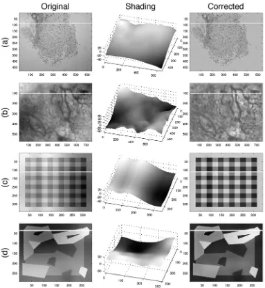
The algorithm was tested on images with different characteristics: a
histological section stained by immunohistochemistry (Fig. 1a), the
vasculature of a tumour from intravital observation (Fig. 1b) and two artificial
images (Fig. 1c,d) with objects of different sizes. While the cells of Fig. 1a
present objects of interest of a relatively small size, the vessels of Fig. 1b
have a larger size and even larger are the chequered squares of Fig. 1c and
the irregular shapes of Fig. 1d. The objects of interest in Fig. 1d are of similar
size and nature as the image that most algorithms failed to correct in [8]. The
images. It should be noted how these surfaces, although slowly varying,
would require a high order polynomial for an accurate approximation. The
right column shows the corrected images. It is noticeable that all the images
now have uniform levels. A profile of each image is presented in Fig. 2. The
left column shows the original shaded image (black line) together with the
envelope (grey discontinuous line). While for Fig. 2a,c the shading
corresponded to Simax, for Fig. 2b,d the shading corresponded to S i
min. In other
words, the background in the first case was considered as bright (high
intensity) while on the second case it was considered dark (low intensity). It is
also important to notice that in the four cases, the shading was corrected as
all the profiles on the right column show uniform intensity levels regardless of
the size of the objects that increase in size from top to bottom.
As an indication of the computational complexity, 28 iterations were required
to process a 342×342 image (Fig. 1c) and the average time was 5.4 s (Matlab
version 7.4.0.287 (R2007a) running on a Mac PowerBook 2.6 GHz Intel Core
2 Duo, 4 GB RAM, OS X 10.5.5). As a comparison, entropy optimisation with
the fminsearch Matlab algorithm of the 10-parameter second order polynomial
proposed in [4] took 45.6 s.
Conclusion
An algorithm based on the envelope detection of image intensities was
presented. The algorithm corrected the shading of different types of images
and did not require the objects of interest to be small in size nor the use of
computationally expensive optimisation algorithms. The spurious intensity
variations were corrected even when the surfaces would not be easily
pre-processing step for segmentation or quantitative analysis and only requires
user intervention to confirm accuracy. This algorithm can be widely used in
biomedical imaging, from microscopy to magnetic resonance.
Acknowledgements
This work was funded by Cancer Research UK.
References
[1] S. Inoué, Video Microscopy. New York: Plenum Press, 1986.
[2] A. L. D. Beckers, W. C. Debruijn, E. S. Gelsema, M. I. Cleton-Soeteman, and H. G. Vaneijk, "Quantitative Electron Spectroscopic Imaging in Bio-Medicine - Methods for Image Acquisition, Correction and Analysis," J Microsc, vol. 174, pp. 171-182, 1994.
[3] J. C. Russ, The Image Processing Handbook, 2nd ed. Boca Raton, FL: IEEE Press, 1995.
[4] B. Likar, J. B. A. Maintz, M. A. Viergever, and F. Pernus, "Retrospective shading correction based on entropy minimization," J Microsc, vol. 197, pp. 285-295, 2000.
[5] A. Simmons, P. S. Tofts, G. J. Barker, and S. R. Arridge, "Sources of Intensity Nonuniformity in Spin-Echo Images at 1.5-T," Magnetic Resonance in
Medicine, vol. 32, pp. 121-128, 1994.
[6] B. Likar, M. A. Viergever, and F. Pernus, "Retrospective correction of MR intensity inhomogeneity by information minimization," IEEE Trans Med Imaging, vol. 20, pp. 1398-1410, 2001.
[7] B. R. Condon, J. Patterson, D. Wyper, P. a. Jenkins, and D. M. Hadley, "Image Nonuniformity in Magnetic-Resonance-Imaging - Its Magnitude and Methods for Its Correction," BJ Radiol, vol. 60, pp. 83-87, 1987.
[8] D. Tomazevic, B. Likar, and F. Pernus, "Comparative evaluation of
retrospective shading correction methods," J Microsc, vol. 208, pp. 212-223, 2002.
[9] Z. J. Hou, S. Huang, Q. M. Hu, and W. L. Nowinski, "A fast and automatic method to correct intensity inhomogeneity in MR brain images," Medical Image Computing and Computer-Assisted Intervention - MICCAI 2006, Pt 2, vol. 4191, pp. 324-331, 2006.
[10] U. Vovk, F. Pernus, and B. Likar, "Intensity inhomogeneity correction of multispectral MR images," Neuroimage, vol. 32, pp. 54-61, 2006.