ILP approaches to the blockmodel problem

ILP Approaches to the Blockmodel Problem

Abstract

Blockmodelling is a method for identifying structural similarities or equivalences between elements which has applications in a variety of contexts, including multiattribute performance assessment. One criterion for forming blocks results in a difficult nonlinear integer pro-gramme. We give several integer linear programming formulations of this problem and provide comparative computational results. We show that methods of reducing symmetry proposed by Sherali and Smith are not effective in this case and propose an iterative approach in which the size of the problem is reduced.

Keywords: integer programming, nonlinear programming, blockmodel, symmetry

1

Introduction

The technique of blockmodelling originated in sociology [?] where it was used principally to identify structural similarities between elements in social networks [?, ?]. More recently it has been used to analyse multiattribute measures of performance in airlines [?], airports [?,?,?] and universities [?]. Blockmodelling provides an alternative to the strict ranking or ‘league table’ approach to relative performance assessment and, it is claimed [?], may have some advantages over the well established technique of data envelopment analysis [?]. In this context the performance, pi, of unit i is assessed via:

pi =

X

j

wjvj(xij)

of units can be obtained. A pair of units can be viewed as having similar performance if the standardised difference between their scores is less than some threshold [?].

Essentially units in the scenario under study are represented by nodes in an undirected graph; an interaction between two units is represented by the presence of an edge between the corresponding nodes. Conventionally there is an edge connecting each node to itself. Two units are structurally similar if they have similar patterns of interaction. The blockmodel concept is to identify a partition of the graph into sets of mutually similar nodes, or blocks. Frequently there will be several possible partitions of the graph so that some means of choosing between them may be desirable. We might require that a block is a complete subgraph, i.e. that nodes in a block are structurally equivalent rather than structurally similar. However this may result in an undesirably large number of blocks. Jessop [?] proposes a criterion, maximum concentration, that favours the formation of a small number of large, dense blocks, i.e. blocks for which the intra-block edge density is close to 1. Justification of this approach and discussion of other approaches is given in [?]. Here we concentrate on the computational aspects of Jessop’s approach.

2

Jessop’s Model and a Transformation

The formulation of the block model problem suggested by Jessop [?] is:

MAX HHI = b

X

k=1 (

n

X

i=1

λik)2

(1)

subject to

b

X

k=1

λik= 1 (i = 1,2,· · · , n) (2)

n

X

i=1 n

X

j=1

xijλikλjk ≥β( n

X

i=1

λik)2

(k = 1,2,· · · , b) (3)

λik = 0 or 1 ∀i, k (4)

chosen to be close to 1. In some circumstances there may be additional con-straints on block sizes. For example, in sociological applications, it may be necessary to prohibit singleton blocks [?]; in design applications [?], maxi-mum block size may be limited. Such constraints can be easily incorporated into the model.

Writing the number of nodes in block k as sk =

Pn

i=1λik, it can be seen that HHI is the sum of squares of block sizes. HHI represents a measure of concentration of the nodes into blocks and clearly favours the formation of a small number of large blocks. It is essentially the same as the Herfindahl-Hirschman Index [?], a popular measure of industrial concentration in an economy. Whenβ = 1, HHI is a multiple of the proportion of edges which are contained within blocks. It seems natural to prefer block structures for which this proportion is higher. Constraints (2) are set partitioning constraints which insist that every node is allocated to a single block. Constraints (3) may be rewritten: _P

n i=1

Pn

j=1xijλikλjk

s2 k

≥β

As Pn_i=1

Pn

j=1xijλikλjk is the number of intra-block edges in block k, the left hand side of this constraint can be seen to represent the edge density of the block. Hence constraints (3) require the edge density of each block to reach a given threshold, β.

The principal difficulty in solving this model is that its continuous relax-ation has a nonconvex feasible region. The direction of optimisrelax-ation com-pounds the difficulty. Thus any attempt to solve this problem by branch and bound requires a global optimisation routine to handle the node subproblems, which potentially is computationally expensive. Commercial mathematical programming systems such as CPLEX, LINGO, MOSEK and XPRESS-MP [?] appear to support the solution of mixed integer quadratically constrained problems only in the convex case. However the binary nature of the variables allows the model to be linearized [?] by replacing the product termλikλjk by a binary variable ωijk together with the logical implications:

λik = 0∨λjk = 0 ⇔ ωijk = 0

ωijk = 1 ⇔ λik= 1∧λjk= 1.

Taking account of the undirectedness of the graph edges, this gives:

MAX HHI = b X k=1 ( n X i=1

λik+ 2 n−1

X

i=1 n

X

j=i+1

subject to

b

X

k=1

λik= 1 (i = 1,2,· · · , n) (6)

2 n−1 X

i=1 n

X

j=i+1

(xij −β)ωijk ≥(β−1) n

X

i=1

λik (k = 1,2,· · · , b) (7)

ωijk≤λik (i = 1,2,· · ·, n−1;j = i+ 1,· · · , n;k = 1,2,· · ·, b) (8)

ωijk≤λjk (i = 1,2,· · · , n−1;j = i+ 1,· · · , n;k = 1,2,· · · , b) (9)

ωijk ≥λik+λjk−1 (i = 1,2,· · · , n−1;j = i+ 1,· · · , n;k = 1,2,· · · , b) (10)

λik = 0 or 1 ∀ i, k; ωijk ≥0 ∀ i, j, k (11)

which we denote Model 1. Note that the variables ωijk can be treated as continuous variables as constraints (8)-(10), together with the nonnegativity of ωijk, force them to be binary in any feasible solution. The price paid for the linearization is a substantial increase in problem size. There are an additional 3bn(n−1)/2 constraints and bn(n−1)/2 variables as compared to the quadratic model (1)-(3). Whilst n is fixed by the problem instance, choice of b is a matter of judgement. We return to this point later.

3

Symmetry Considerations

The model detailed in Section 1 exhibits symmetry in that the labelling (1, 2, · · ·, b) of the blocks, whilst necessary for the specification of the model, is in reality arbitrary. Given a feasible allocation of nodes to blocks, any permutation of the block labels will also give a feasible solution. Symmetry is known to cause significant difficulties in tree search algorithms for the solution of discrete optimisation problems. Discussion and examples are given, for example, in Proll [?] and Sherali and Smith [?] in the case of integer linear programming, Proll and Smith [?] and Smith et al. [?] in the case of constraint programming, and Petrie et al. [?] in the case of hybrid constraint programming/linear programming.

are allocated to a particular block, which is what we need to know. Hence we employ the second approach.

An ordering of the blocks can be induced by insisting that they are in-dexed in nonincreasing order of size. This can be implemented by adding the constraints:

n

X

i=1

λi1 ≥ n

X

i=1

λi2 ≥ · · · ≥ n

X

i=1

λib. (12)

With this ordering, we can also impose:

n

X

i=1

λi1 ≥ ⌈n/b⌉. (13)

We denote the augmented model Model 2.

In their work on the SONET problem, Sherali and Smith also suggested the use of:

n

X

i=1

iλi1 ≥ n

X

i=1

iλi2 ≥ · · · ≥ n

X

i=1

iλib (14)

as a means of distinguishing between symmetric arrangements. In this case, suppose that, for example, we have an allocation in which nodes 1 and 2 are (fully) allocated to block i and nodes 3 and 4 are allocated to block

j (j < i). For simplicity suppose that all other nodes are distributed across the remaining blocks, Then (12) allows this solution and also a solution in which nodes 3 and 4 are allocated to block i and nodes 1 and 2 to block j, the distribution of other nodes remaining unchanged. Such solutions are not allowed by (14). As there are frequently many solutions containing blocks of the same size, there is some hope that (14) might be more effective than (12) in reducing the effects of symmetry. We denote the model comprising (1)-(11) and (14) as Model 3.

4

Computational Experiments

Computational experiments on Models 1, 2 and 3 were performed on seven problem instances ranging in size from 20 to 47 nodes using CPLEX 8.1 on a 2.8GHz processor running under Fedora Core 4 Linux. The parameter β

time over 1 million nodes had been explored, the number of active nodes was still increasing at a substantial rate and the integrality gap was still 65%. The same problem was allowed to run to proven optimality using Model 2; a process which took in excess of 131 hours. Clearly the branch and cut search has to be a truncated one. A maximum cpu time limit of 600 secs was set for problems 1-3 and 900 secs for problems 4-7.

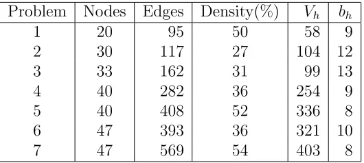
Jessop [?] describes a constructive heuristic for the blockmodel problem in the case β = 1. This was used to determine the maximum number of blocks, b, to be considered for each problem instance. Table 1 shows the problem data and the results obtained with the heuristic, where Vh is the HHI value attained and bh is the corresponding number of blocks.

Problem Nodes Edges Density(%) Vh bh

1 20 95 50 58 9

2 30 117 27 104 12

3 33 162 31 99 13

4 40 282 36 254 9

5 40 408 52 336 8

6 47 393 36 321 10

7 47 569 54 403 8

Table 1: Problem data and heuristic solutions

Problem 1 arises from an analysis of the results of a particular season in the Barclays Premier League, the top division in English soccer [?]. Problem 2 arises from elective choices in an MBA programme [?]. Problem 3 is taken from a study of dwellings within a city [?]. Problems 6 and 7 arise from a multicriteria assessment of airport performance [?]; problems 4 and 5 are subsets of problems 6 and 7 respectively.

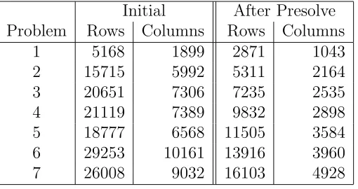
Table 2 shows that the potentially large MILP model is substantially re-duced by CPLEX Presolve [?]. The reason for the magnitude of the reduction is clear. The insistence that the blocks are fully dense (β = 1) implies that if nodes i and j are not connected by an edge they cannot be in the same block. Hence the variablesωijk and associated constraints can be deleted, or indeed not generated. This will not be the case for other values of β.

Initial After Presolve Problem Rows Columns Rows Columns

1 5168 1899 2871 1043

2 15715 5992 5311 2164

3 20651 7306 7235 2535

4 21119 7389 9832 2898

5 18777 6568 11505 3584 6 29253 10161 13916 3960 7 26008 9032 16103 4928

Table 2: Problem size

Best Upper

Problem V0 V1 HHI No Ne Na Bound 1 210.00 210.00 78 5904 20411 1974 152 2 264.00 262.50 128 2843 3721 307 224 3 357.00 355.92 117 0 1271 344 325 4 604.00 602.55 276 1592 1619 341 543 5 856.00 855.00 340 273 928 301 782 6 833.00 833.00 337 390 461 154 798 7 1185.00 1185.00 505 440 579 183 1111

Table 3: Results for Model 1

In Table 3, V0 is the objective value of the LP relaxation, V1 is the ob-jective value after the addition of cuts, Best HHI is the obob-jective value of the best integer feasible solution found, No is the number of the node at which this solution was found, Ne is the number of nodes explored prior to termination, Na is the number of active nodes remaining at termination.

The LP relaxation is clearly quite weak and not much improved by CPLEX cuts, despite there being of the order of 200 - 400 cuts generated at the root node. Nor are these cuts effective at later nodes. Progress in the search is characterized by a slow rate of reduction in the upper bound. The experiments suggest that it is relatively easy to find feasible solutions, a high proportion of which are found by CPLEX’s heuristic.

to run their instances of the SONET problem to proven optimality. This is not the case for the problem studied here as the search necessarily has to be truncated because of the observed slow progress towards proven optimality.

Model 2 Model 3

Best Best

Problem V0 V1 HHI V0 V1 HHI

1 210.00 208.14 78 210.00 208.41 70 2 264.00 260.40 110 264.00 261.45 -3 357.00 355.63 107 357.00 355.48 89 4 604.00 601.40 238 604.00 601.81 216 5 856.00 854.81 246 856.00 853.97 294 6 833.00 831.12 283 833.00 831.45 321 7 1185.00 1183.08 367 1185.00 1183.73 355

Table 4: Results for Models 2 and 3

Sherali and Smith observed that CPLEX’s heuristic finds it much more difficult to find feasible solutions when the symmetry breakers are present, particularly early on in the search. The experiments reported here echo this. A feasible solution of Model 1 was found at the root node for each problem and, in four of the seven cases, was better than that found by Jessop’s heuristic. A first feasible solution of Models 2 and 3 was never found at the root node and, for the larger problems in particular, took a significant amount of the limited search time to find, for example Model 2 took 542 seconds to find a first IFS for problem 6. For each problem, the solution found was worse than that found by Jessop’s heuristic. This goes some way to explaining why the use of the symmetry breakers does not appear beneficial in a truncated search. Trick [?] discusses other reasons why tightening the LP relaxation of an ILP at the modelling stage may not be beneficial.

consistently improve because of the cutoff.

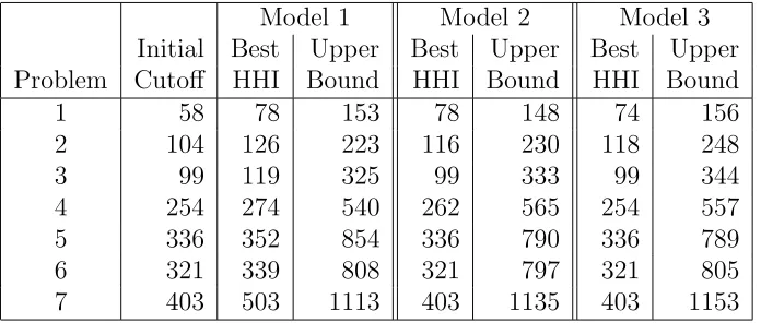
Model 1 Model 2 Model 3 Initial Best Upper Best Upper Best Upper Problem Cutoff HHI Bound HHI Bound HHI Bound

1 58 78 153 78 148 74 156

2 104 126 223 116 230 118 248

3 99 119 325 99 333 99 344

4 254 274 540 262 565 254 557

5 336 352 854 336 790 336 789

6 321 339 808 321 797 321 805

7 403 503 1113 403 1135 403 1153

Table 5: Results with Cutoffs Imposed

Thus our experience reinforces the warnings of Ragsdale and Shapiro [?] that use of such cutoffs may, in fact, degrade performance of a branch and cut search, particularly when the search is truncated.

Table 5 also shows that Models 2 and 3 are not especially successful in decreasing the upper bound on the objective function compared to Model 1. Table 6 shows the progress of Models 1 and 2 on problem 2 at approximately 600 second intervals. Progress on the other problems is similar and does not suggest that the symmetry breaking constraints become more beneficial when the search is less truncated.

Model 1 Model 2 Model 1 Model 2 no initial cutoff with initial cutoff Time Best Upper Best Upper Best Upper Best Upper (secs) HHI Bound HHI Bound HHI Bound HHI Bound

0 98 262 - 261 104 262 104 261

600 128 224 110 225 126 223 116 230 1200 128 219 114 219 126 216 116 217 1800 136 215 122 215 126 212 128 214 2400 136 211 128 212 126 209 128 210 3000 136 208 128 208 128 206 128 207 3600 136 206 132 207 128 204 128 205

Table 6: Progress of Models 1 & 2 on Problem 2

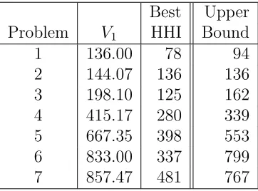
and to add symmetry breaking cuts to an MILP model. By default this option is switched off, as was the case for the experiments described earlier. Table 7 displays results for Model 1 with this option switched on. The results show that the CPLEX symmetry cuts are effective in tightening the LP relaxation of Model 1, resulting in substantially decreased initial upper bounds in all but problem 6. Better values of the objective function are obtained for problems 2 - 5, including a proven optimal solution to problem 2, but a worse value for problem 7. The case of problem 6 is a strange one as CPLEX does not detect a symmetry pattern even though one obviously exists. There do not appear to be any features of problem 6 that clearly distinguish it from the other problems which might explain this behaviour. Note also that the presence of these symmetry breaking cuts does not affect the ability of CPLEX’s heuristic to find an IFS at the root node in every case.

Best Upper Problem V1 HHI Bound

1 136.00 78 94

2 144.07 136 136 3 198.10 125 162 4 415.17 280 339 5 667.35 398 553 6 833.00 337 799 7 857.47 481 767

Table 7: Results for Model 1 with Symmetry Preprocessing

5

Alternative Approaches

As any solution of Model 1 is a partition of a fixed number of nodes into distinct blocks, the HHI value of a solution, which is a quadratic function of block size, will tend to increase as the number of blocks decreases. It is easily shown that an upper bound on HHI for a problem with n nodes and exactly

b blocks is (n−b + 1)2

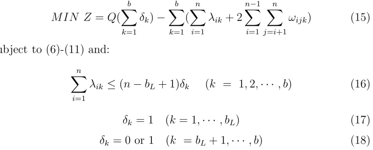
of blocks. One approach is to introduce variablesδkrepresenting the presence (δk = 1) or absence (δk = 0) of block k and to replace (5)-(11) by:

MIN Z =Q( b

X

k=1

δk)− b

X

k=1 (

n

X

i=1

λik+ 2 n−1

X

i=1 n

X

j=i+1

ωijk) (15)

subject to (6)-(11) and:

n

X

i=1

λik ≤(n−bL+ 1)δk (k = 1,2,· · ·, b) (16)

δk = 1 (k= 1,· · · , bL) (17)

δk= 0 or 1 (k =bL+ 1,· · ·, b) (18)

where bL is a lower bound on the number of blocks. We denote this Model 4. Unless the edge density of the graph is at least β, in which case the problem is trivial, bL ≥ 2. Setting Q = n2 + 1 gives pre-emptive priority to minimising the number of blocks [?]. Results for Model 4 under similar conditions to those used in the experiments with Model 1 recorded in Table 3 are given in Table 8. The only change to the conditions was that the branching strategy gave priority to the δ variables over the λ variables and, within the δ variables, to the down direction, i.e. to eliminating a block.

Problem V0 V1 Blocks Best HHI

1 1145.97 1795.40 6 78

2 8136.02 8191.59 10 136

3 7471.90 8378.33 10 125

4 8160.87 12204.00 8 280

5 5952.31 8027.63 6 390

6 12909.30 19057.00 9 353

7 8615.57 12075.00 6 519

Table 8: Results for Model 4

For Model 4, the CPLEX default cut strategy is much more effective, both at the root node, as indicated in Table 8, and throughout the search. Model 4 finds the same solution as Model 1 for problem 1 but gives a better solution on termination for all the other problems.

by Jessop’s heuristic. The relatively good results provided by Model 4 sug-gest that looking for solutions with a small number of blocks is productive. Disaggregating (15) gives a two stage process, firstly minimising the number of blocks via Model 5 and then maximising HHI via Model 1. This has some advantage in that the search space for Model 1 is reduced by the elimination of n(n−1)/2 constraints and n+n(n−1)/2 variables for a reduction of 1 in b. Model 5 is:

MIN

b

X

k=1

δk (19)

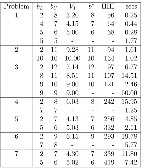
subject to (6)-(11), (15)-(17). It is run iteratively to allow the bounds bL, b on the number of blocks to be revised. The procedure is:

Set bL = 2, b=bh, terminate = false While not terminate do

Solve Model 5 If Model 5

(i) proves no IFS exists, terminate = true (ii) finds an IFS with b∗ _blocks

b ←b∗₋₁

bL← ⌈V1⌉

(iii) does not find an IFS,bL← ⌈V1⌉ If bL =b∗ terminate = true

Solve Model 1

Problem bL bU V1 b∗ HHI secs

1 2 8 3.20 8 56 0.25

4 7 4.15 7 64 0.44 5 6 5.00 6 68 0.28

5 5 - - - 1.77

2 2 11 9.28 11 94 1.61 10 10 10.00 10 134 1.02 3 2 12 7.14 12 97 6.77 8 11 8.51 11 107 14.51 9 10 9.00 10 121 2.46 9 9 9.00 - - 60.00 4 2 8 6.03 8 242 15.95

7 7 - - - 1.25

5 2 7 4.13 7 256 4.85

5 6 5.03 6 332 2.11 6 2 9 6.15 9 293 19.78

7 8 - - - 5.77

7 2 7 4.30 7 339 11.80 5 6 5.02 6 419 7.42

Table 9: Sequential bound determination

In Table 9, aV1 value of - denotes that the LP relaxation is infeasible, a

b∗ _{value of - denotes that it is proven that no IFS exists within the bounds}

on the number of blocks. In most cases an IFS is found without branching. Table 10 gives the results obtained in the final run of Model 1 with the maximum number of blocks to be formed determined as above.

After Presolve Best Upper

Problem Rows Columns V0 V1 b HHI Bound

1 1910 690 210.00 207.65 6 78 117

2 4430 1470 264.00 257.83 10 136 224 3 5573 1950 357.00 353.44 10 125 316 4 8744 2576 604.00 600.50 8 280 540 5 8638 2688 856.00 852.67 6 390 680 6 13628 3960 833.00 831.12 9 363 781 7 11963 3696 1185.00 1182.06 6 519 1028

The best HHI values found by this procedure are the same as those tained from Model 4 except for problem 6 for which a better solution is ob-tained. In addition, the best solution is generally found considerably earlier in the search.

The block modelling problem described here is essentially an optimisation problem on a graph. As such it is related to a number of other well-studied graph optimisation problems, such as maximal clique, minimum colouring or maximal independent set [?]. When β = 1 a block is precisely a clique. Further, the problem addressed by Model 5, finding the minimum number of blocks, is equivalent to finding a minimum colouring of the complement of the graph. Hence it may seem productive to explore this relationship. However objective function (19) is a coarse one which potentially admits many optimal solutions, whereas objective function (1) has more discriminatory power. Use of (19) here is simply as an aid to the primary objective of maximising HHI. Moreover methods for solving the graph optimisation problems referred to above do not appear to extend to the block modelling problem with β <1. We prefer to explore here methods which are applicable to both cases.

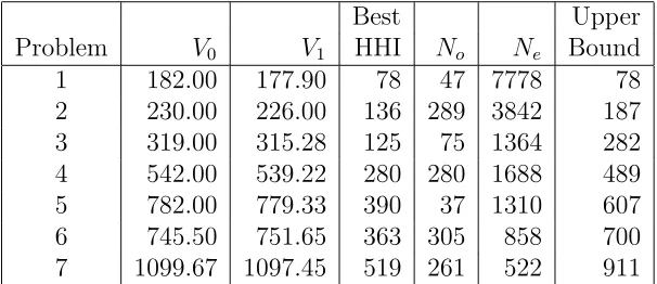
In a further attempt to reduce the effect of symmetry, following the dis-appointing performance of Models 2 and 3, the same device as in [?] was used to remove some of the arbitrariness in the labelling of the blocks. This can be done by insisting that block 1 contains one of the nodes of maximal degree, further reducing the size of the ILPs. We denote as Model 6 the model comprising Model 1 with the maximum number of blocks determined by the iterative use of Model 5 and with block 1 partially specified in this way. Table 11 shows the results from Model 6.

Best Upper

Problem V0 V1 HHI No Ne Bound 1 182.00 177.90 78 47 7778 78 2 230.00 226.00 136 289 3842 187 3 319.00 315.28 125 75 1364 282 4 542.00 539.22 280 280 1688 489 5 782.00 779.33 390 37 1310 607 6 745.50 751.65 363 305 858 700 7 1099.67 1097.45 519 261 522 911

Table 11: Results from Model 6

88 secs. Although no better solutions are found for the remaining problems, useful reductions in both the initial and final upper bounds are obtained.

Table 12 shows the effect of combining Model 6 and Model 2, i.e. making a partial assignment to block 1 and adding constraints similar to (12) for blocks 2, . . . , b and confirms the earlier finding that these constraints do not help if the search is truncated. Worse solutions pertain at termination for three of the four largest problems.

Best Upper

Problem V0 V1 HHI No Ne Bound 1 182.00 177.90 78 126 4878 78 2 230.00 223.90 136 780 2295 172 3 319.00 313.58 125 680 1023 283 4 542.00 540.12 274 302 997 496 5 782.00 779.41 390 444 690 600 6 745.50 752.79 333 355 432 710 7 1099.67 1096.67 507 299 434 932

Table 12: Results from Model 6 combined with Model 2

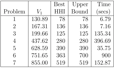
As Table 13 shows, the combination of Model 6 with CPLEX’s symme-try preprocessor allows the search to be completed for all problems except problem 6, for which symmetry is again not detected.

Best Upper Time Problem V1 HHI Bound (secs)

1 130.89 78 78 6.79

2 167.31 136 136 7.16 3 199.66 125 125 135.34 4 437.62 280 280 396.69 5 628.59 390 390 35.75 6 751.65 363 700 900 7 855.00 519 519 152.87

Table 13: Results for Model 6 with Symmetry Preprocessing

As remarked earlier, it is possible that a better solution exists with a larger number of blocks than considered in Model 6, even if the solution found by Model 6 is ‘proven optimal’. This is evidenced by comparing the result for problem 5 in Table 13 with that in Table 7. However the approach described here offers a way of getting a good solution in reasonable time. Obtaining a proven optimal solution to instances of the block model problem is likely to be very expensive. For example, by using the approach described here, we know that the best HHI value we can obtain for problem 1 with most 6 blocks is 78. The upper bound on HHI for a 13 block solution is 76. Hence to confirm or deny that the optimal HHI value for problem 1 is 78 would require looking at solutions with between 7 and 12 blocks. Attempts to do so using Model 6 with the addition of the constraints:

n

X

i=1

λik ≥1 (k= 1,· · · ,7)

were abandoned without result after 20 hours. Even proving that there is no better solution in exactly seven blocks took in excess of two hours.

6

The Case of Non-Full Density Blocks

When β < 1 the block density constraints (3) are weaker than when β = 1. Consequently we expect that there are likely to be many more feasible partitions of each graph and a correspondingly larger search space. Also, as noted earlier, the reductions achieved by presolve will not be as great as is the case when β = 1. Additionally preliminary investigations showed that CPLEX’s cuts were again ineffective and that, surprisingly, CPLEX’s heuristics are not as effective in finding feasible solutions as for the full density block case. These factors may make it more difficult to find good partitions in a limited time. In recognition of this, the time limits on the branch and cut search were increased to 1200 secs for Problems 2-3 and 1800 secs for Problems 4-7.

any feasible solution to the full block case is a feasible solution to the cor-responding non-full block case and can potentially be improved as follows. Suppose i, j are full density blocks withsi, sj members respectively and that there are eij edges connecting nodes in block i to nodes in block j. The number of blocks can be reduced by 1 if:

s2 i +s

2

j + 2eij ≥β(si+sj) 2

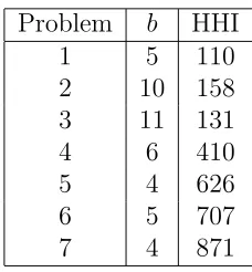
as blocks i and j can be merged. Successive block mergers yield the results in Table 14.

Problem b HHI

1 5 110

2 10 158 3 11 131

4 6 410

5 4 626

6 5 707

7 4 871

Table 14: Results from Heuristic for β = 0.8

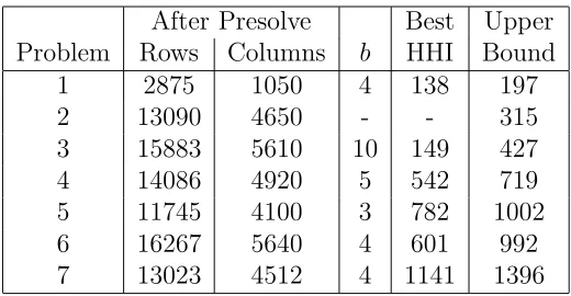
Unfortunately the increased size of the subproblems and the inability of the CPLEX heuristics to find feasible solutions early enough in the search causes the procedure for reducing the number of blocks to be considered, described in Section 5, to be ineffective. With the exception of Problem 1, for which a 4 block solution was found, no feasible solutions or other useful information was found within the imposed time limits of 90 secs for problems 1-3 and 120 secs for problems 4-7. We can, of course, use the number of blocks provided by the procedure for β = 1, which is relatively cheap to compute, if this improves on the number of blocks found by the heuristic for any value

After Presolve Best Upper Problem Rows Columns b HHI Bound

1 2875 1050 4 138 197

2 13090 4650 - - 315

3 15883 5610 10 149 427

4 14086 4920 5 542 719

5 11745 4100 3 782 1002

6 16267 5640 4 601 992

7 13023 4512 4 1141 1396

Table 15: Results from Model 1 for β = 0.8

The results achieved in Table 15 suggest that satisfactory results can be obtained from Model 1 if the initial number of blocks is low. They are much worse if the number of blocks is high, as is the case for Problems 2 and 3; this is partly due to the relatively low density of the graph for these problems.

Table 16 gives the results obtained when a node of maximum degree is ‘anchored’ in block 1. Unlike the case of β= 1, the results with the anchored model do not weakly dominate those of the unanchored model; worse values of HHI being obtained for Problems 3 and 4 whilst a better value is obtained for Problems 5 and 7. Each of the models fails to find a feasible solution in one case. Adding either of the symmetry breaking constraints (12) or (14) again is not beneficial to performance.

After Presolve Best Upper Problem Rows Columns b HHI Bound

1 2065 760 4 138 179

2 12219 4350 10 162 278 3 14922 5280 10 141 401

4 13383 4680 5 540 658

5 8943 3120 3 806 909

6 15576 5405 - - 936

7 12470 4324 4 1141 1305

Table 16: Results from anchored Model 1 for β = 0.8

in three of the other cases and, in the remaining three, worse solutions were obtained.

Best Upper Problem HHI Bound

1 138 138

2 - 273

3 - 162

4 450 658

5 782 916

6 - 936

7 1069 1278

Table 17: Results for anchored Model 1 for β = 0.8 with Symmetry Preprocessing

Although better HHI values are obtained via ILP for those problems for which feasible solutions are found, the failure of the ILP approaches to always find feasible solutions is problematic.

7

Conclusions

The results given in Table 11 suggest that, despite the weakness of the LP relaxation, ILP does provide a means of getting substantially better qual-ity solutions to full-densqual-ity problems of up to 50 nodes than does Jessop’s heuristic in a reasonable amount of time. Larger problems may well be prob-lematic unless some problem specific cuts can be developed to tighten the LP relaxation. This is even more important for the non-full density block problem as the size of the resulting ILP may make it difficult to find good solutions, even if only a small number of blocks need be formed. Finding good solutions to the non-full density remains challenging.

8

Acknowledgements

I am grateful to Alan Jessop for helpful discussions, provision of data and for supplying me with the code for his heuristic. I am also grateful to the anonymous referees whose comments and suggestions were most helpful.

References

[1] NEOS Optimization Software Guide. http://www-fp.mcs.anl.gov/otc/Guide/SoftwareGuide/, November 2004.

[2] I P Gent and B M Smith. Symmetry breaking during search in constraint programming. In W Horn, editor,Proceedings of ECAI-2000, pages 599– 603. IOS Press, 2000.

[3] A Jessop. Multiple attribute probabilistic assessment of the performance of some airlines. In M Koksalan and S Zionts, editors, Multiple Criteria Decision Making in the New Millenium, pages 417–426. Springer, Berlin, 2001.

[4] A Jessop. Exploring structure: a blockmodel approach. Civil Engineer-ing and Environmental Systems, 19:263–284, 2002.

[5] A Jessop. Blockmodels with maximum concentration. European Journal of Operational Research, 148:56–64, 2003.

[6] K E Petrie, B M Smith, and N Yorke-Smith. Dynamic symmetry break-ing in constraint programmbreak-ing and linear programmbreak-ing hybrids. Tech-nical Report APES-81-2004, Apes Research Group, University of St An-drews, 2004.

[7] L G Proll. Formulation of integer linear programs - an example. Inter-national Journal of Mathematical Education in Science and Technology, 20:415–420, 1989.

[8] L G Proll and B M Smith. ILP and constraint programming ap-proaches to a template design problem. INFORMS Journal on Com-puting, 10:265–275, 1998.

[10] H D Sherali and J C Smith. Improving discrete model representations via symmetry considerations. Management Science, 47:1396–1407, 2001.