Solving Many Objective Car Sequencing Problems on Two Sided Assembly Lines Using an Adaptive Differential Evolutionary Algorithm

Article

Solving Many-Objective Car Sequencing Problems on

Two-Sided Assembly Lines Using an Adaptive

Differential Evolutionary Algorithm

Parames Chutima

_{and Trirat Kirdphoksap}

1 Department of Industrial Engineering, Faculty of Engineering, Chulalongkorn University, Bangkok 10330, Thailand

2 Regional Centre for Manufacturing Systems Engineering, Chulalongkorn University, Bangkok 10330, Thailand

3 The Royal Society of Thailand

E-mail: a_{[email protected] (Corresponding author),} b_{[email protected]}

Abstract. The car sequencing problem (CSP) is addressed in this paper. The original environment of the CSP is modified to reflect real practices in the automotive industry by replacing the use of single-sided straight assembly lines with two-sided assembly lines. As a result, the problem becomes more complex caused by many additional constraints to be considered. Six objectives (i.e. many objectives) are optimised simultaneously including minimising the number of colour changes, minimising utility work, minimising total idle time, minimising the total number of ratio constraint violations and minimising total production rate variation. The algorithm namely adaptive multi-objective evolutionary algorithm based on decomposition hybridised with differential evolution algorithm (AMOEA/D-DE) is developed to tackle this problem. The performances in the Pareto sense of AMOEA/D-DE are compared with COIN-E, MODE, MODE/D and MOEA/D. The results indicate that AMOEA/D-DE outperforms the others in terms of convergence-related metrics.

Keywords: Car sequencing, two-sided assembly line, many objectives, evolutionary algorithm, decomposition, differential evolutionary algorithm.

ENGINEERING JOURNAL Volume 23 Issue 4 Received 24 September 2018

1.

Introduction

A car sequencing problem (CSP) has attracted much attention from car manufacturers and researchers for many decades. The CSP practised by automotive manufacturers was first elaborated in a scientific manner by Parrello, et al. [1]. The classical version of the CSP consists in establishing the daily launching order of a set of cars with different types and options (e.g. sunroof, a navigation system, camera, etc.) to be produced on the mixed-model final assembly line to achieve a predefined goal without violating capacity constraints. The CSP can be broadly viewed as a subset of the job shop scheduling problem.

RENAULT, the renowned French car manufacturer, articulated in the 2005’s ROADEF challenge that the CSP in a modern car factory must consider three major shops rather than taking into account just the constraints and objectives related to the assembly shop like in the classical CSP. These three shops ordered sequentially include the body fabrication shop where the chassis of the cars are produced, the paint shop where the cars are painted by workers and robots, and the assembly shop where different options are installed in the cars [2]. Moreover, most car manufacturers put great efforts in the order-taking process to please customers by shortening production lead time and offering a large variety of options.

The CSP is a strong NP-hard problem. The CSP was used to consider as a constraint satisfaction problem in which different priorities could be given to the constraints. Recently, Kis [3] demonstrated that the problem was rather well-match with a combinatorial optimisation problem, even the ratio-constraint alone was taken into account. Adding more constraints involving in the body fabrication shop and paint shop into the classical CSP enhances the complexity of the problem dramatically. The brute force approaches of constraint programming or integer programming may not be effective enough to solve the problem since the software could reach its limit when facing practical-sized problems [4].

Gagné, et al. [5] argue that the production equipment such as robots installed in the body fabrication shop is flexible enough to adjust its output rate to match with the demands given by the other two manufacturing shops. As a result, to reduce the complexity of the CSP, the constraints from the body fabrication shop could be neglected since their impacts on the daily car sequencing plan are not significant. In other words, the optimal solution obtained from solving the CSP in which taken into consideration only the objectives and constraints of the paint shop and assembly shop is sufficient to reflect the operations of the car production facility as a whole [6].

Most research on the CSP normally attempts to optimise only a single objective. However, in reality, various objectives are applicable and they should be optimised simultaneously. Moreover, the layout of the assembly line used in the traditional model is simplified by adopting the straight-shaped form. The assumption as such is unpractical because the car size is big which normally needs two workers to work on the opposite sides of the workstation to assemble different components on the same car to shorten line length and improve operations efficiency. Moreover, task times and precedence relationships of various car models are disregarded in the traditional model. Consequently, the capacity problem involved in the necessity of utility workers employed to help clear up all unfinished tasks leftover by regular workers is ignored.

Recently, a more practical platform of the CSP was proposed by Chutima and Olarnviwatchai [7]. The major modifications given to the traditional model included using the two-sided assembly line (2SAL) to replace the straight-shaped assembly line (or the one-sided assembly line, 1SAL), explicitly considering precedence relationships and task times of different car models, and optimising multi-objectives simultaneously. This modified model was called “a car sequencing problem on the two-sided assembly line (CSP2SAL)”.

The remaining of this paper is organised as follows. A comprehensive review related to CSP and 2SAL is elaborated in Section 2. The distinct characteristics of the MaCSP2SAL are discussed in Section 3. Section 4 explains the proposed algorithm (AMOEA/D-DE) to solve the MaCSP2SAL, followed by Section 5 that shows the experimental design. The experimental results and concluding remarks are given in Sections 6 and 7, respectively.

2.

Literature Review

2.1. CSP

The CSP has attracted attention from practitioners and researchers for many decades since it paves the way for the advanced studies of formulations and solution searching strategies. The CSP was first formally elaborated by Parrello, et al. [1]. Initially, the CSP was formulated through a constraint satisfaction model to find an optimal sequence of different car models manufactured along an assembly line without violating contiguity constraints, while satisfying their demands. However, in practice, more appropriated formulation of the CSP should be a combinatorial optimisation problem rather since some of their constraints could be violated, but with additional penalty cost [6, 9].

The CSP was proved to be in the class of NP-hard combinatorial optimisation problems [3, 10]. As a result, the exact solution to large-scaled CSPs is difficult to achieve. Solnon, et al. [11] presented a comprehensive review of the exact and heuristic approaches for solving the CSP. It was indicated that the approaches that could provide a relatively good solution fairly quickly were more practical and useful than those that achieved an optimal solution at the expense of irrational computational time. Hence, unsurprisingly, various approximated solution approaches such as heuristics or metaheuristics became dominated in the good solution searching process of the CSP.

Warwick and Tsang [9] classified the CSP into two types, i.e. solvable and unsolvable (no solution). In addition, previous research on the CSP was mainly emphasised on the solvable problem. However, the CSP should rather be considered as a partial constraint satisfaction problem in which constraints could be violated but at some predetermined cost. A generic genetic algorithm (GAcSP) in which the repair and hill climbing mechanisms were combined with the genetic algorithm (GA) to find the solutions of both solvable and unsolvable CSPs. Jaszkiewicz, et al. [12] described an adaptation of the genetic local search algorithm (GLS) in which a systematic approach to the construction of recombination operators, a heuristic for efficient initial solution creations, and a fast local search method was developed.

Smith, et al. [13] formulated the CSP using a nonlinear integer programming and proposed two heuristics, i.e. steepest descent and simulated annealing (SA), and Hopfield neural network to solve the problem approximately. Briant, et al. [14] tackled the CSP via SA. The dynamic probabilities taken into account the best success rate of each move so far were used to find predominant neighbours for the given instance.

Puchta and Gottlieb [15] compared three permutation-based local search algorithms which employed different acceptance criteria for moves. Two variants of threshold accepting approaches were superior to the greedy approach to solution quality and robustness. Prandtstetter and Raidl [2] proposed a new integer linear programming (ILP) formulation for small- and medium-sized CSP instances. For the large-sized problem, a general variable neighbourhood search (VNS) approach encompassed the large neighbourhoods examined using ILP technique were shown promising. Two local search approaches, i.e. very large neighbourhood search and very fast local search, were compared by Estellon, et al. [4]. They mentioned that sophisticated metaheuristics were impractical to solve the CSP. Ribeiro, et al. [16], Ribeiro, et al. [17] approximately solved the CSP using a set of heuristics based on the paradigms of the VNS and iterated local search (ILS) metaheuristics which were further enhanced with the intensification and diversification strategies. The optimised data structure for the effective implementation of heuristics was also proposed.

Gottlieb et al. [6] compared a few heuristics used in the CSP, i.e. greedy heuristics, local search and ant colony optimisation (ACO). It was revealed that the ACO outperformed the others in obtaining better solution quality for smaller time limits. Gagné, et al. [5] developed the ACO as a new and powerful solution engine which contained effective transition rules for solving a multi-objective CSP. Solnon [18] introduced an ACO working under two different pheromone structures, each of which aimed at learning for good car sequences or learning for critical cars. Since the operations of these pheromone structures were complementary to each other, their combination could significantly improve the algorithm speed.

et al. [20] developed an iterated TS heuristic which combined the classical TS with perturbation operators in order to avoid the local optima.

Zinflou, et al. [21] introduced three new crossover operators using with a GA to solve the CSP, i.e. interest based crossover (IBX), uniform interest crossover (UIX) and non-conflict position crossover (NCPX). Zinflou and Gagné [22] proposed an algorithm, which is a hybridisation of a GA and an artificial immune system, namely GISMOO, to tackle the multi-objective CSP in a Pareto sense. The Pareto solutions obtained from GISMOO dominated those of the non-dominated sorting genetic algorithm (NSGA II) and Pareto memetic strategy for multiple-objective optimisations (PMSMO_{). Atiker et al. [23] proposed a heuristic} to tackle the CSP under the scenario in which high priority ratio constraints are primary, and colour constraints are secondary.

2.2. 2SAL Sequencing

Prior to launching orders to the assembly line, the assembly sequence of parts and subassemblies must be determined. Bahubalendruni and Biswal [24] reviewed and discussed research articles on the assembly sequence generation published over the past four decades. Obviously, an appropriate assembly sequence results in minimal lead time and low cost of assembly [25].

The mixed-model assembly line sequencing problem has been one of the research topics that challenges researchers during the last decade. Obviously, most research was mainly conducted on one-sided straight-shaped assembly lines. This environment is applicable to small-sized products, e.g. printed circuit board, television, etc. where each worker is comfortable to work effectively with a workpiece and its assembly components. Since the size of cars is too big to manipulate by a single worker, two-sided assembly lines where two workers perform their assigned tasks cooperatively in a workstation tend to be a more effective alternative for doing assembly works.

Boysen et al. [26] give a detailed review of mixed-model sequencing algorithms and illustrated a number of potential performance measurements commonly used in literature, e.g. workload variation, part usage rate variation, amount of utility work, etc. In addition, most research in the early years attempted to optimise only a single objective such as the articles of Miltenburg, et al. [27] and Stiener and Yeomans [28].

During the last decade, the trend of the research has moved towards multi-objective optimisation of mixed-model sequencing problems which much more reflects the decision maker’s point of view in practice. The challenging issue arises from several objectives to be optimised simultaneously are often conflict with one another; therefore, a compromised solution becomes implicitly acceptable. In addition, Pareto-based solution techniques are more appropriate than weighted sum techniques [29].

A new constraint occurred in the 2SAL, but not in the 1SAL, is sequence-dependent finish time of tasks. Since two workers have to work concurrently and cooperatively on the same workpiece in a mated station of 2SAL, the finish time of tasks done by one worker could affect the start time of tasks to be performed by the other. As a result, to find the optimal operations of the CSP2SAL, the launching sequence of mixed-model cars and the cooperation of workers in the same mated station must be contemplated carefully.

Since the CSP2SAL is NP-hard by nature, the evolutionary algorithm seems to be promising solution techniques. Several researchers employed this algorithm to solve the 2SAL sequencing problem including TS [30], Pareto stratum-niche cubicle genetic algorithm [31], SA [32], genetic algorithm [33], ant colony optimisation [34], memetic algorithm [35], multi-objective scatter search [36], coincidence algorithm [37], extended coincidence algorithm [7], etc.

3.

Problem Definition

According to the proposal in the ROADEF’05 challenge on the CSP, the car production facility in industry consists of three main steps serially interconnected as the body fabrication shop, paint shop and assembly shop [2]. Car chassis, metal fabrication, bodywork and welding process are manufactured in the body fabrication shop. Various predefined colours are painted on the bodies of cars according to customer orders in the paint shop. In the assembly shop, engine, suspension parts, electrical parts, underbody parts as well as specific options, e.g. sunroof, alloy wheel, sports seat, satellite navigation, etc. are installed into the car.

which must be taken into account in optimising the CSP are limited to the paint shop and the assembly shop only [6].

As mentioned earlier, the CSP should be considered as a combinatorial optimisation problem rather than a constraint satisfaction problem since in practice their constraints could be violated. When a constraint is violated, the number of occurrences in a particular type will be notified and accumulated. Cordeau, et al. [20] recommended that some types of violations happening in a certain production day 𝐽 were affected by the actual production in the previous day (𝐽 − 1) and the planned production in the next day (𝐽 + 1). As a result, these three consecutive days must be considered all together to effectively assess the constraint violations.

Two constraints are normally emphasised in the CSP, i.e. ratio constraint (𝑅𝐶) and number of paint colour changes (𝑁𝐶𝐶). The 𝑅𝐶, a capacity related constraint, is the primitive constraint of the traditional CSP. The simplified version of this constraint is formalised by a ratio 𝑝 𝑞⁄ meaning that for each particular option at most 𝑝 cars could be installed with that option in any subsequence production segment of 𝑞 cars. The 𝑅𝐶 is a soft constraint meaning violations are feasible but with a cost. Ribeiro, et al. [16], Ribeiro, et al. [17] subdivided the 𝑅𝐶 into two categories, i.e. high and low priorities. The low priority 𝑅𝐶 has the value of the 𝑅𝐶 less than the high priority 𝑅𝐶. In fact, the option with high priority 𝑅𝐶 will impose heavy workload on the assembly line and demonstrating the sense of production difficulty.

To count the number of 𝑅𝐶 violations, the sliding window method is normally used. This method counts all 𝑅𝐶 violations whenever found (Gottlieb et al. 2003). However, this method does not only double counting the 𝑅𝐶 violations, but also it could be biased by the violations occurring around the beginning and the end of the daily production sequence. To mitigate this issue, Fliedner and Boysen [37] suggested counting only the actual number of occurrences leading to the 𝑅𝐶 violations. An numerical example is demonstrated in Chutima and Olarnviwatchai [7].

Another constraint of the CSP recently introduced by the ROADEF challenge is the number of colour change (𝑁𝐶𝐶). This constraint occurred in the paint shop where various colours are painted on the bodies of cars. Since unproductive setups are inevitable when changing paint colours from one to another, cars should be painted with the same colour in a batch as many as possible. However, the maximum batch size (𝐶𝐵𝑆_𝑚𝑎𝑥) is controlled by two events, i.e. number of cars continuously painted with the same colour before the paint gun agglutinates and before visual colour inspection becomes ineffective, depending on which one is less. Obviously, 𝐶𝐵𝑆𝑚𝑎𝑥 is a hard constraint; hence, any car sequence that violates the 𝐶𝐵𝑆𝑚𝑎𝑥 is

unfeasible. To count the 𝑁𝐶𝐶 correctly, the colour of the last car produced in day 𝐽 − 1 must be compared with the first car of day 𝐽 to check if the colour change is occurred or not.

Most literature published on the CSP always assumes that one-sided assembly lines (1SALs) are used in the assembly shop which is unrealistic in practice. The more pragmatic assumption is the utilisation of 2SALs. Recently, Chutima and Olarnviwatchai [7] introduced the new version of the CSP where the 2SAL was employed in the system namely the CSP2SAL. In their research, apart from the 𝑅𝐶 and 𝑁𝐶𝐶, the utility work (𝑈𝑇𝑊) arisen due to the employment of the 2SAL was also optimised. This research extends the previous work of Chutima and Olarnviwatchai [7] to include more pragmatic objectives related to the 2SAL and just-in-time production environment called MaCSP2SAL. Feasible solutions of the MaCSP2SAL is a permutation of daily car production sequence in which all hard constraints are satisfied and the violations of the soft constraints are minimised.

In this research, six objective functions normally used in automotive industry and literature are optimised simultaneously to assess the effectiveness of the car sequence in 2SAL including minimising number of colour changes, minimising utility work, minimising total idle time, minimising number of RC violations, minimising total production rate variation and minimising total parts usage variation. The detailed formulation of each objective is elaborated as follows.

𝑓₁=minimise 𝑁𝐶𝐶 = ∑𝑛𝑐−1𝛿_{𝐶𝑂𝐿𝑘,𝑘+1}

𝑘=0 (1)

where

𝑘 position of the car sequence in day 𝐽, (𝑘 ∈ [1, 𝑛𝑐])

𝑛𝑐 number of the cars to be produced in day 𝐽

𝐶𝑂𝐿_𝑘 colour of the car located at the position 𝑘

𝛿_{𝐶𝑂𝐿𝑘,𝑘+1} difference in colours of cars in positions 𝑘 and 𝑘 + 1, (𝛿_{𝐶𝑂𝐿𝑘,𝑘+1}= 1 if the colours of cars in positions 𝑘 and 𝑘 + 1 are different; and 0 otherwise)

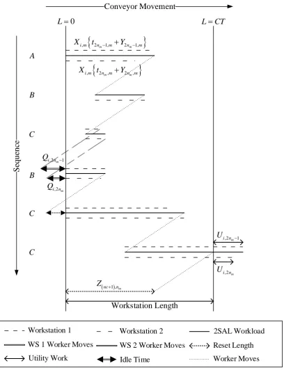
(b) Minimising utility work (𝑈𝑇𝑊): In 2SAL, the utility work represents the unfinished tasks leftover by regular workers due to the cycle time limitation. Utility workers have to help complete these unfinished utility works to avoid line stoppage and allow the worker in the next workstation to start his operation at the earliest start time. The pictorial explanation is in Fig. 1. The second objective can be formulated as follows [38].

𝑓₂=minimise 𝑈𝑇𝑊 = ∑ (∑𝑛𝑐 𝑈_{𝑖,𝑛𝑚}+ 𝑍_{(𝑖+1),𝑛𝑚}

𝑖=1 /𝑠𝑐)

𝑁𝑀

𝑛𝑚=1 (2)

subject to

𝑈𝑖,𝑛𝑚= {

max[0,(𝑍𝑖,𝑛𝑚+𝑠𝑐∑𝑀𝑚=1𝑋𝑖,𝑚{𝑡2𝑛𝑚−1,𝑚+𝑌2𝑛𝑚−1,𝑚}−𝐿𝑛𝑚)

𝑠𝑐 ]

+max[0,(𝑍𝑖,𝑛𝑚+𝑠𝑐∑𝑀𝑚=1𝑋𝑖,𝑚{𝑡2𝑛𝑚,𝑚+𝑌2𝑛𝑚,𝑚}−𝐿𝑛𝑚)

𝑠𝑐 ]

} (3)

𝑍_{(𝑖+1),𝑛𝑚}=

max{max[0,min(𝑍𝑖,𝑛𝑚+ 𝑠𝑐∑ 𝑋𝑖,𝑚{𝑡2𝑛𝑚−1,𝑚+ 𝑌2𝑛𝑚−1,𝑚} 𝑀

𝑚=1 − 𝛾𝑠𝑐, 𝐿𝑛𝑚− 𝛾𝑠𝑐)]

,max[0,min(𝑍_{𝑖,𝑛𝑚}+ 𝑠_𝑐∑𝑀 𝑋_𝑖,𝑚{𝑡_{2𝑛𝑚,𝑚}+ 𝑌_{2𝑛𝑚,𝑚}}

𝑚=1 − 𝛾𝑠𝑐, 𝐿𝑛𝑚− 𝛾𝑠𝑐)]

} (4)

where

𝑛_𝑚 sequential number for each mated station (𝑛_𝑚 = 1, 2, …, 𝑁_𝑀)

𝑛𝑐_𝑣 number of cars in model 𝑣 ∈ 𝑉 to be produced in the current day

𝑛𝑐 total daily production order (𝑛𝑐 = ∑𝑉 𝑛𝑐_𝑣

𝑣=1 )

𝛾 rate of the product launch interval into the conveyer

𝑡_𝑗,𝑣 total operation time for car model 𝑣 at station 𝑗

𝑌_𝑗,𝑣 total unavoidable idle time caused by the sequence-dependent finish time of tasks for car model 𝑣 at station 𝑗

𝑠_𝑐 conveyor speed

𝐶𝑇 cycle time of the line

𝐿𝑛𝑚 fixed line length of the mated station 𝑛𝑚 (𝐿𝑛𝑚 = 𝑠𝑐∗ 𝐶𝑇)

𝑈_{𝑖,𝑛𝑚} amount of utility work required for the 𝑖th product (𝑖 = 1 … 𝐼) in a sequence at the mated station 𝑛_𝑚

𝑋_𝑖,𝑣 existent of car model 𝑣 at the 𝑖th product sequence (𝑋_𝑖,𝑣= 1, if the 𝑖th car in a sequence is model 𝑣; and 𝑋𝑖,𝑣= 0, otherwise)





, 2 m 1, 2 m 1,

i m n m n m

X t _ Y _

0

L LCT





, 2 _m, 2 _m,

i m n m n m

X t Y

,2 m 1

i n

U _

,2 _m

i n U

,2 _m 1

i n

Q _

,2 m

i n Q

nc 1 ,n_m

Z _

Workstation Length

A

B

C

C B C

S

eque

nc

e

Workstation 1 Workstation 2 2SAL Workload

WS 1 Worker Moves WS 2 Worker Moves Reset Length

Utility Work _{Idle Time} Worker Moves

Conveyor Movement

(c) Minimising total idle time (𝐼𝑇): In 2SAL, the duration which the worker has to wait before the next car entering the workstation is to be minimised in order to increase worker utilisation. Since two workers are needed in the mated stations of 2SAL, the total idle time of this kind is the sum of the idle time from each worker. The pictorial explanation is illustrated in Fig. 1. The third objective can be formulated as follows [39].

𝑓3=minimise 𝐼𝑇 =_𝑣1

𝑐∑ ∑ 𝑄𝑖,𝑛𝑚

𝑛𝑐 𝑖=1

𝑁𝑀

𝑛𝑚=1 (5)

𝑄_{(𝑖+1),𝑛𝑚} = {max[0, 𝛾𝑠𝑐− (𝑍𝑖,𝑛𝑚+ 𝑠𝑐∑ 𝑋𝑖,𝑚{𝑡2𝑛𝑚−1,𝑚+ 𝑌2𝑛𝑚−1,𝑚}

𝑀

𝑚=1 )]

+ max[0, 𝛾𝑠_𝑐− (𝑍𝑖,𝑛𝑚+ 𝑠𝑐∑ 𝑋𝑖,𝑚{𝑡2𝑛𝑚,𝑚+ 𝑌2𝑛𝑚,𝑚}

𝑀

𝑚=1 )]

} (6)

subject to

𝑠_𝑐∑𝑀 𝑋_𝑖,𝑚{𝑡_{2𝑛𝑚−1,𝑚}+ 𝑌_{2𝑛𝑚−1,𝑚}}

𝑚=1 > 0 ∀𝑖∀𝑛𝑚 (7)

𝑠_𝑐∑𝑀 𝑋_𝑖,𝑚{𝑡_{2𝑛𝑚,𝑚}+ 𝑌_{2𝑛𝑚,𝑚}}

𝑚=1 > 0 ∀𝑖∀𝑛𝑚 (8)

where

𝐼𝑇 total idle time to wait for the next car entering the mated stations

𝑄𝑖,𝑛𝑚 distance before the 𝑖th car sequence to enter the mated station 𝑛𝑚

(d) Minimising a total number of RC violations (𝑇𝑁𝑅𝐶𝑉): In the assembly shop, the same standard body of cars could be installed with different options to satisfy the personalised demands of specific customers. For some difficult-to-install options, workers have a limited capacity to handle such heavy workload continuously before feeling tired. Therefore, these options have to distribute uniformly along the production sequence so that workers can reduce their fatigues by installing difficult options alternatively with those easy ones. The RC of the option 𝑜 ∈ 𝑂 is defined as 𝑝_𝑜⁄𝑞_𝑜 meaning that for any segment with length 𝑞_𝑜 of the car production sequence, at most 𝑝_𝑜 cars requiring option 𝑜 to be produced. Obviously, for an easy option the ratio of 𝑝_𝑜⁄𝑞_𝑜 is low. Because the subsequent segment of 𝑞_𝑜 cars must be considered in the RC violation, the last 𝑞_𝑜− 1 cars produced in day 𝐽 − 1 and the first 𝑞_𝑜− 1 cars produced in day 𝐽 + 1 must be used in determining the RC violation in day 𝐽. Since the RC is a soft constraint, violations are possible but at a cost. The modified sliding window technique proposed by Fliedner and Boysen [16] is used in this research since it can count the actual positional occurrences of violations effectively. Besides revealing the number of violations correctly without double counting, this technique could reveal the maximum number of overloaded workstations also. The fourth objective can be formulated as follows (note: a calculation sample can be seen in [7]).

𝑓4=minimise 𝑇𝑁𝑅𝐶𝑉 = ∑𝑜∈𝑂{𝑁𝑃𝑉𝑜; 𝑖 𝜖 𝑑𝑎𝑦 𝐽}⟦⋃𝑛𝑐𝑖=−𝑞0+1𝑃𝑉𝑜(𝑖, … , 𝑖 + 𝑞𝑜− 1)⟧} (9)

where

∪ union set operator

𝐽 current production day

𝑛𝑐 number of cars to be produced in day 𝐽

𝑃𝑉_𝑜(𝑖, … , 𝑖 + 𝑞𝑜− 1) set of positions where violations occurred under a sliding window starting

from position 𝑖 to 𝑖 + 𝑞_𝑜− 1

𝑁𝑃𝑉_{𝑜; 𝑖 𝜖 𝑑𝑎𝑦 𝐽}}⟦ ⟧ number of positions only in day 𝐽 in which violations occurred for option 𝑜

𝑓₅=minimise 𝑃𝑅𝑉 = ∑ ∑ |(∑ 𝑋𝑙,𝑚

𝑖 𝑖

𝑙=1 ) −𝑑_𝑛𝑐𝑚|

𝑀 𝑚=1 𝑛𝑐

𝑖=1 (8)

where

𝑚 car models to be produced by the assembly line (𝑚 = 1, …, 𝑀)

𝑑_𝑚 demand of the car model 𝑚

𝑛𝑐 number of cars to be produced in the current day

𝑋𝑙,𝑚 existent of car model 𝑚 at the 𝑙th product sequence (equal to 1 if car 𝑙th in the assembly

sequence is of model 𝑚, and 0 otherwise)

(f) Minimising total parts usage variation (𝑃𝑈𝑉): In the assembly shop, the parts usage variation directly affects the preparation of parts for each product model to be assembled in the assembly line. If parts usage variation is high or parts consumption is uneven, the production planning will become difficult and the possibility of parts shortage is high. The sixth objective can be formulated as follows [40].

𝑓₆=minimise 𝑃𝑈𝑉 = ∑ ∑ (𝑖×𝑁𝑗

𝑛𝑐 − 𝑈𝑇𝑗,𝑖)

2 𝛽

𝑗=1 𝑛𝑐

𝑖=1 (9)

𝑈𝑇_𝑗,𝑖= ∑ ((∑𝑖 𝑋_𝑙,𝑚

𝑙=1 ) × 𝑏𝑚,𝑗) 𝑀

𝑚=1 (10)

𝑁_𝑗= ∑𝑀 (𝑑_𝑚× 𝑏_𝑚,𝑗)

𝑚=1 (11)

where

𝛽 number of parts variety

𝑁_𝑗 total quantity of part 𝑗 required by all cars

𝑑_𝑚 demand of car model 𝑚

𝑈𝑇𝑗,𝑖 total number of part 𝑗 being assembled from the first product sequence until 𝑖th product

sequence (𝑖 = 1, … , 𝑛𝑐; 𝑗 = 1,2, … , 𝛽)

𝑏_𝑚,𝑗 number of units of part 𝑗 required per unit of car model 𝑚 (equal to 1 if car model 𝑚 uses part 𝑗; 0 otherwise)

4.

Proposed Solution Approach

4.1. AMOEA/D-DE

The CSP has long been considered as a multi-objective optimization problem (MOP) in practice since various conflicting objectives may need to be achieved simultaneously by car manufacturers. Previously, due to the absence of advanced metaheuristic theories as well as computer hardware and software, the multi-objective CSP had to be solved as a single objective optimisation by defining an aggregate utility function which takes a weighted sum of various objectives or alternatively solving these multi-objectives in a lexicographic order based on their preferential priorities. However, during the past two decades, the concepts of evolutionary algorithms and Pareto optimality have become more acceptable among researchers resulting in simultaneously optimising objectives used in the CSP under more realistic production environment is realisable [7].

According to Coello and Zacatenco [41], the formal formulation of the MOP is as follows.

𝑚𝑖𝑛𝑖𝑚𝑖𝑠𝑒 𝐹(𝒙) = (𝑓1(𝒙), 𝑓2(𝒙), … , 𝑓𝑚(𝒙)) 𝑇 (12)

subject to 𝒙 𝜖 𝑅𝑛

where 𝒙 = (𝑥1, 𝑥2, … , 𝑥𝑛)𝑇 is the vector of decision variables located in the feasible landscape of 𝑅𝑛, and 𝑓𝑖(𝒙) is the value of the 𝑖th objective function (𝑖 = 1,2, … , 𝑚) in the objective space of 𝑅𝑚. Due to the

A solution 𝒙 is said to dominate a solution 𝒚 (mathematically written as 𝒙 ≺ 𝒚) if 𝒙 is not worse than 𝒚

in any objective and at least in one objective 𝒙 is strictly better than 𝒚. However, if 𝒙 is better than 𝒚 in one or more objectives and 𝒚 is better than 𝒙 in one or others, these two solutions are non-dominated (indifferent) to each other. Moreover, we said that 𝒙 is a Pareto optimal solution (POS) or an efficient solution if 𝒙 is non-dominated over the set of solutions under consideration. The vector of POSs plotted in the objective space forms the Pareto front (PF). The ideal PF should contain a reasonable number of POSs, all of which are diverse and spread uniformly throughout the whole area of the objective space.

One of the effective approaches to tackle the MOP is the application of multi-objective evolutionary algorithms (MOEAs) since the shape or discontinuity of PFs affects their performance very little. Most conventional MOEAs employ POSs to guide their search trajectories to improve the fitness of the solutions. However, this approach may be ineffective particularly in case of more than three objectives (i.e. many objectives) are dealt with simultaneously. When the number of the objectives escalates, the number of POSs will increase accordingly due to the lessening of the Pareto domination strength among the obtained solutions [42].

A novel MOEA to solve many-objective optimisation problems (MaOPs) was proposed by Zhang and Li [58] namely a multi-objective evolutionary algorithm based on decomposition (MOEA/D). The algorithm was found to perform very well on a number of MOPs. The MOEA/D decomposes the original MaOP into a number of subproblems in which different single objectives formulated by the scalar aggregations of uniformly distributed weight vectors are assigned to each of them. Unlike Pareto-based MOEAs, these diverse weight vectors are the key parameter used in projecting the search direction of the algorithm towards the optimal solution. In each generation, these subproblems are collaboratively optimised simultaneously. After the evolutionary process completes, the optimal solution to each of these subproblems is brought together to form the PF of the original MaOP.

To generate weight vectors for subproblems in the MOEA/D, the simplex-lattice design, a conventional decomposition method of the mixture experimental design, is often used. Let 𝑚 be the number of objectives to be simultaneously optimised, 𝑖 = (₁𝑖_{, … ,}

𝑚

𝑖 ₎𝑇 _{be a weight vector of the 𝑖th subproblem (where } 𝑗𝑖≥ 0

for all 𝑗 = 1, …, 𝑚; and ∑𝑚 _𝑗𝑖

𝑗=1 = 1). The number of subproblems (i.e. population size 𝑁𝑝) in the (𝑚, 𝐻)

simplex-lattice design in which each objective takes 𝐻+1 equally distanced between 0 and 1 is 𝐶_{𝐻+𝑚−1}𝑚−1 _.

The MOEA/D utilises the information from each subproblem and its neighbourhoods to improve the fitness of solutions. Let 𝐵𝑖_(𝑁

𝑛) be a set of neighbourhood sized 𝑁𝑛 of the 𝑖th subproblem. The

subproblems {𝑖₁, 𝑖₂, … , 𝑖_𝑁𝑛} belong to the neighbourhood of the subproblem 𝑖 if the Euclidean distances between their weight vectors 𝑖1_,𝑖2_{, … ,}𝑖𝑁𝑛 _{and the weight vector }𝑖 _{are shortest comparing with the rest.}

Since the values of 𝑖 of the subproblem 𝑖 and their neighbourhoods are not much different and closely related, the solutions within this area tend to have quite similar characteristics and hence they are used as a mechanism to guide searching direction towards the optimal solution.

Although various approach could be used to transform many objectives in the subproblems of the original MOP into scalar single-objective optimization problems, the Tchebycheff approach seems to be more effective because of its computational simplicity and effectiveness in handling non-convex PF [43]. The Tchebycheff function 𝑔(𝑥) is expressed as follows.

min 𝑔(𝑥|𝑖_{, 𝑧}∗_{) = 𝑚𝑎𝑥}

1≤𝑗≤𝑚{𝑗𝑖|𝑓𝑗(𝑥) − 𝑧𝑗∗|} (13)

where 𝑥 is the decision variable, Ω is the feasible region of the decision variable 𝑥, 𝑓_𝑗(𝑥) is the real value of the 𝑗th objective, 𝑧∗ _{= (𝑧}

1∗, … , 𝑧𝑚∗)𝑇 is a utopian point, and 𝑧𝑗∗= 𝑚𝑖𝑛{𝑓𝑗(𝑥)|𝑥 ∈ Ω} is the reference point

(i.e. so-far best value of the 𝑗th objective). The function {𝑗𝑖|𝑓𝑗(𝑥) − 𝑧𝑗∗|} is the weighted absolute deviation

between the value of the 𝑗th objective and its reference point. The Tchebycheff function attempts to reduce the highest weighted absolute deviation of the subproblem as much as possible.

𝑓̅_𝑗= 𝑓𝑗−𝑧𝑗∗

𝑧𝑛𝑎𝑑_−𝑧

𝑗∗ (14)

where 𝑓̅_𝑗 is the normalised value of the 𝑗th objective, and 𝑧𝑛𝑎𝑑 _{= 𝑚𝑎𝑥{𝑓}

𝑗(𝑥)|𝑥 ∈ 𝑃𝑂𝑆} is the nadir point

in the objective space.

In order to create new tentative solutions (offspring), the original version of the MOEA/D uses the genetic operator, i.e. one point crossover, which is normally used in the GA. However, the GA was outperformed by the differential evolution (DE) algorithm in terms of global search ability [44, 45]. Li and Zhang [46], Li and Zhang [47] proposed a multi-objective differential evolution based decomposition (MODE/D) in which the genetic operator was replaced by the differential operators and revealed that the MODE/D performed better than several other MOEAs on many test problems.

The DE, a subset of evolutionary algorithms, was first introduced by Storn [48] for global optimisation problems over continuous-valued landscapes. The DE has been recognised as a simple yet effective algorithm for successfully implemented in many engineering practices, e.g. power generation, engineering design, etc. [49]. The DE uses a real number to represent each variable in the solution. To produce tentative offspring, two of DE’s operators are applied to solutions in the current generation in the order of mutation first and then crossover. The mutation operator creates a trial vector for each individual parent by mutating each variable in a target vector with a weighted differential of different vectors. After that, the crossover operator manipulates discrete recombination between the trial vector and the parent vector to form a new offspring. The fitness of the offspring is compared with its parent to determine which one will be survived in the next generation.

Various DE strategies, in which the main differences are on mutation and crossover operators, have been developed in the literature [50]. To articulate their variations, a general notation as DE/𝑥/𝑦/𝑧 is normally adopted; where 𝑥 is the target vector selection method, 𝑦 is the number of difference vectors used in the mutation, and 𝑧 is the crossover method. The MODE/D uses the DE/rand/1/bin strategy to create offspring which works as follows. Under the conventional MOEA/D platform, for each individual subproblem 𝑖th (i.e. parent vector 𝒙_𝑖 ), three solutions are selected from the population (i.e. the neighbourhood of the subproblem, 𝐵𝑖_(𝑁

𝑛)) at random. One of them (𝒙𝑟1) acts as a target vector (𝑥 = rand)

and the remaining twos (𝒙𝑟2 and 𝒙𝑟3) are used to find the differential variation (𝑦 = 1). The mutant vector

𝒗𝑖 is computed by perturbing the target vector with the weighted differential as follows.

𝒗𝑖= 𝒙𝑟1+ 𝐹(𝒙𝑟2− 𝒙𝑟3) (15)

where 𝒗_𝑖 is the mutant vector of the parent vector 𝒙_𝑖 (𝑖 ≠ 𝑟₁≠ 𝑟₂ ≠ 𝑟₃) and 𝐹 ∈ (0, ∞) is the scale factor. Once the mutation is finished, the crossover operator creates the trial vector 𝒙_𝑖′ _{from the recombination of}

the mutant vector 𝒗𝑖 and its target vector (parent) 𝒙𝑖. For the binomial crossover (𝑧 = bin) which is normally

used in literature, the crossover points are randomly selected from the set of feasible crossover points 𝑗 ∈ [1, 𝑛𝑥] as follows.

𝑥_𝑖,𝑗′ _{= {}𝑣𝑖,𝑗, if 𝑟𝑎𝑛𝑑𝑜𝑚[0,1] < 𝐶𝑅 or 𝑗 = 𝑗𝑟𝑎𝑛𝑑𝑜𝑚

𝑥_𝑖,𝑗, otherwise (16)

where 𝒙_𝑖′ _{is the trial vector, 𝑥}

𝑖,𝑗′ , 𝑣𝑖,𝑗 and 𝑥𝑖,𝑗 are the 𝑗thelement of the vectors 𝒙𝑖′, 𝒗𝑖 and 𝒙𝑖, respectively, 𝑛_𝑥 is the number of elements in the vector, and 𝐶𝑅 is the crossover probability. Obviously, the higher the value of 𝐶𝑅, the more element of the mutant vector will be included in the offspring than the parent (base vector), and vice versa. To ensure that at least one element of the trial vector is distinct from its parent, the crossover point 𝑗𝑟𝑎𝑛𝑑𝑜𝑚 is randomly selected and assigning the value of 𝑣𝑖,𝑗𝑟𝑎𝑛𝑑𝑜𝑚 to 𝑥𝑖,𝑗𝑟𝑎𝑛𝑑𝑜𝑚

′ _{. The}

polynomial mutation is applied to the initial mutation vector to become the (final) mutation vector 𝒙_𝑖′′ _{in the}

following way [49].

𝑥_𝑖,𝑗′′ _{= {}𝑥𝑖,𝑗′ + 𝜎𝑛(𝑥𝑖,𝑗′𝑈𝑝− 𝑥𝑖,𝑗′𝐿𝑤) with probability 𝑝𝑚 𝑥_𝑖,𝑗′ _{with probability 1 − 𝑝}

𝑚

𝜎_𝑛= {(2 × 𝑟𝑎𝑛𝑑𝜎)

1

𝜂+1_{− 1 if 𝑟𝑎𝑛𝑑}

𝜎< 0.5

1 − [2(1 − 𝑟𝑎𝑛𝑑_𝜎)]𝜂+11 _otherwise

(18)

where

𝑥_𝑖,𝑗′𝑈𝑝 the lower bound of the 𝑗th_{element of the vectors 𝒙} 𝑖 ′

𝑥_𝑖,𝑗′𝐿𝑤 _{the lower bound of the 𝑗}th_{element of the vectors 𝒙} 𝑖 ′

𝑟𝑎𝑛𝑑_𝜎 random number sampling from a uniform distribution [0, 1]

𝑝_𝑚 mutation probability

𝜂 distribution index of polynomial mutation

Once a trial vector is created, its fitness is compared with its base vector’s fitness and the one with better fitness will be survived as an offspring of the DE operations.

Apart from the DE strategy, the behaviour of the algorithm could be controlled by other parameters including population size, mutation factor 𝐹 and crossover probability 𝐶𝑅. If the population size is big, a large number of individuals will participate in the mutation resulting in a greater chance to create a better offspring. The mutation factor 𝐹 affects the searching ability of the DE in generating potential trail vectors. The values of 𝐹 directly affect the search landscape of the DE, i.e. local search for small 𝐹 values and global search for large 𝐹 values. Moreover, the crossover probability 𝐶𝑅 controls the proportion of elements in the offspring to be inherited from the trial vector or the parent. The offspring is more resemble to the trial vector than the parent if the values of 𝐶𝑅 is high, and vice versa.

Conventionally, the DE strategy, as well as the values of the control parameters, are determined beforehand and they are kept unchanged during the course of the evolutionary search. As a result, the same searching pattern is repeatedly applied regardless of current fitness landscape causing a high risk of being trapped in local optima. In fact, the processes to obtain an appropriate DE strategy and the best values for individual control parameters are laborious. Although prior knowledge from previous research (if any) may be a good starting point for finding appropriate control parameter settings, a trial-and-error investigation which requires tedious experimental trials is necessary for the tuning process since these control parameters are mostly problem dependent. Moreover, the DE strategies and the values of the corresponding control parameters that make the algorithm perform best in one stage of the evolutionary search may not be preferred in another stage [51]. This shortcoming could be overcome by embedding an adaptive mechanism in the main structure of the algorithm.

Zhang and Sanderson [52] categorised parameter control mechanisms into three classes, i.e. deterministic, adaptive and self-adaptive. While the adaptive and self-adaptive parameter controls take feedback information from the evolutionary process to dynamically update the control parameters, the deterministic parameter control simply uses some deterministic rules to adjust the control parameters. The adaptive and self-adaptive parameter controls differ in that the latter uses a method of the evolution of evolution through mutation and crossover in the self-adaptation of control parameters. If the adaptive or self-adaptive parameter control is well planned, the robustness of the algorithm could be strengthened. Besides no tiresome trial-and-error trail is needed, the convergence rate of the algorithm could be improved when allowing the values of its control parameters to be dynamically updated to suit various search characteristics at different stages of the evolutionary process.

The DEs with adaptive or self-adaptive mechanism showed faster and more reliable convergence than those without [53, 54]. Among them, the randomisation-adaptation based DE usually outperforms the others [55]. Specifically, the randomisation-adaptation based DE uses some forms of probability distribution function, whose probability is derived from the successful offspring generation rate, to randomly provide various appropriate values of the control parameters, i.e. 𝐹 and 𝐶𝑅. In this research, the concept of randomisation-adaptation based DE is adopted under the framework of MODE/D, namely AMOEA/D-DE, to solve the MaCSP.

mutation strategy adaptation, and (2) control parameter adaptation. The detail of each mechanism is explained as follows.

Mutation strategy adaptation: AMOEA/D-DE adapts the concept of simultaneous implementation of multi-mutation strategies from SaDE [53]. Three mutation strategies (𝑠1, 𝑠2 and 𝑠3) are in the candidate pool to allow the algorithm to generate a variety of search patterns with respect to the current requirement of the fitness landscape. As a result, at generation 𝑔, a trial vector 𝒗_𝑖,𝑔 can be generated by one of these strategies.

𝑠1: DE/rand/1: 𝒗𝑖,𝑔= 𝒙𝑟1,𝑔+ 𝐹(𝒙𝑟2,𝑔− 𝒙𝑟3,𝑔) (19)

𝑠2: DE/rbest/1: 𝒗𝑖,𝑔= 𝒓best𝑖,𝑔+ 𝐹(𝒙𝑟1,𝑔− 𝒙𝑟2,𝑔) (20)

𝑠3: DE/rand-to-rbest/1: 𝒗𝑖,𝑔= 𝒙𝑟1,𝑔+ 𝛾(𝒓best𝑖,𝑔− 𝒙𝑟1,𝑔) + 𝐹(𝒙𝑟2,𝑔− 𝒙𝑟3,𝑔) (21)

These mutation strategies are chosen in this research since they are simple to implement, widely used in DE literature, and reported to perform well on diverse problems. The mutation strategy DE/rand/1 is quite robust in generating diverse solutions but in contrast, its convergence rate is quite slow since it searches around a relatively small landscape without bias towards any particular direction. Gämperle et al. [56] indicated that the utilisation of the information from the best solution in developing a trial vector, e.g. DE/best/1, could be beneficial in fast convergence by focusing the search in the vicinity of the best solution. However, this strategy may cause premature convergence from reduced population diversity. To alleviate the weak point of fast but less reliable convergence, the mutation strategy DE/rand-to-best/1 which is the blending between DE/rand/1 and DE/best/1 is developed so that the trial vector could gain mutual benefits from both mutation strategies by searching around a wider landscape and biasing its searches towards potential optimum directions.

Under the base structure of MOEA/D, the vector located at a particular position in the neighbourhood of subproblem 𝑖 currently being the best-so-far solution that subproblem 𝑖 has ever found till generation 𝑔

could be replaced by another solution during the evolutionary process of generation 𝑔. As a result, in generation 𝑔+1, the information on the real best solution of subproblem 𝑖 will be lost if such replacement occurs in generation 𝑔 especially with a poorer solution. Therefore, the information of the best-so-far solution associated with subproblem 𝑖 must be constantly updated and kept throughout the evolutionary process. Moreover, in order to find the real best (𝒓best) of subproblem 𝑖 to be used in Eq. (18) and (19), its best-so-far solution must also be taken into account along with the solutions in the neighbourhood in the competition arena. Where 𝒓best = (𝑟best₁, 𝑟best₂, … , 𝑟best_𝑛𝑥)𝑇

The mutation strategy adaptation of the AMOEA/D-DE is modified from Qin and Suganthan [50] to suit the context of MaCSP. Initially, the selection probability of each strategy is set to be equal (1/3). After completing the evolutionary process in each generation, the number of trial vectors successfully and unsuccessfully surviving in the next generation by each mutation strategy is recorded. In addition, the number of survival trial vectors becoming new non-dominated solutions is also counted. This information is used to update the probabilities of strategy selection in the next generation as follows.

𝑝_𝑠,𝑔+1= 𝑝_𝑚𝑖𝑛+ (1 − 𝑆 × 𝑝_𝑚𝑖𝑛) ∙ [(1 − 𝛼)𝑝𝑠,𝑔+ 𝛼 ∙ (_∑𝑆𝑆𝑢𝑐_𝑆𝑢𝑐𝑠,𝑔_𝑠,𝑔

𝑠=1 )] (22)

𝑆𝑢𝑐𝑠,𝑔 =_𝑛𝑠𝑛𝑠𝑠,𝑔

𝑠,𝑔+𝑛𝑓𝑠,𝑔 (23)

𝑛𝑠𝑠,𝑔 = ∑ ∑𝑁𝑗=1𝑛 𝐷𝑆𝑅𝑖,𝑗,𝑔𝑠

𝑁𝑝

𝑖=1 (24)

𝑛𝑓𝑠,𝑔 = ∑ ∑𝑁𝑗=1𝑛 (1 − 𝑆𝑅𝑖,𝑗,𝑔𝑠 ) 𝑁𝑝

𝑖=1 (25)

where

𝑠 selectable strategy, 𝑠∈{𝑠1, 𝑠2, 𝑠3}

𝑆 total number of selectable strategy (𝑆 = 3 in this research)

𝑁_𝑝 population size

𝑁_𝑛 neighborhood size

𝑝_𝑠,𝑔 probability of selecting strategy 𝑠 in generation 𝑔

𝑝𝑚𝑖𝑛 minimum probability of selecting any strategy (𝑝𝑚𝑖𝑛 = 0.05 in this research)

𝑆𝑢𝑐𝑠,𝑔 proportion of strategy 𝑠 successfully creating survival offspring vectors in generation 𝑔 𝑛𝑠_𝑠,𝑔 number of strategy 𝑠 successfully creating survival offspring vectors in generation 𝑔 𝑛𝑓_𝑠,𝑔 number of strategy 𝑠 unsuccessfully creating survival offspring vectors in generation 𝑔

𝑆𝑅_{𝑖,𝑗,𝑔}𝑠 number of strategy 𝑠 successfully creating offspring vector that are better than the parent

vector and its neighboring solutions of subproblem 𝑖 (𝑆𝑅_{𝑖,𝑗,𝑔}𝑠 _{= 1, if the offspring vector 𝒙} 𝑖 ′′

is better than its parent vector 𝒙_𝑖 and the other neighboring vectors 𝒙_𝑗 of subproblem 𝑖 in generation 𝑔; 0, otherwise)

𝐷𝑆𝑅_{𝑖,𝑗,𝑔}𝑠 _{number of strategy 𝑠 successfully creating offspring vector that are better than the parent}

vector and its neighbouring solutions of subproblem 𝑖, and the offspring vector becoming a new non-dominated solution (𝑆𝑅_{𝑖,𝑗,𝑔}𝑠 = 1, if the offspring vector 𝒙_𝑖′′ is better than its parent vector 𝒙𝑖 and the other neighboring vectors 𝒙𝑗 of subproblem 𝑖, and the offspring vector

becoming a new non-dominated solution in generation 𝑔; 0, otherwise)

The detailed numerical example of MOEA/D-DE to solve MaCSP2SAL is given in [57].

Control parameter adaptation: The control parameters used in the DE could affect the convergence rate and diversity exploration performances significantly. As mentioned earlier, the values of the control parameters should not be fixed but allowed to vary based on the progress step and direction of the current search requirement. The first DE control parameter the value of which is adjusted during the evolutionary process is the mutation factor 𝐹 which is a key parameter used for generating mutant vectors. The values of 𝐹 have a direct impact to the exploitation and exploitation performances of the algorithm. A relatively small 𝐹

renders fast convergence rate but may lead to premature convergence.

The concept to adjust 𝐹 in this research is adapted from Zhang and Sanderson [52]. At each generation, the mutation factor of each subproblem 𝑖 is independently updated based on a Cauchy distribution depending on the number of successful offspring creations in the previous generation. The Cauchy distribution is used because it could diversify 𝐹 to avoid premature convergence especially in greedy mutation strategies as DE/rbest/1 and DE/rand-to-rbest/1. The formulation is as follows.

𝐹_𝑖,𝑔+1𝑠 = {Cauchy(𝜇𝐹,𝑖,𝑡+1

𝑠 _{, 0.1), if 𝑟𝑎𝑛𝑑}

1< 𝜏𝑖,𝑔𝑠

𝐹_𝑖,𝑔𝑠 _{, otherwise} (26)

𝜇_{𝐹,𝑖,𝑔+1}𝑠 _{= {}(1 − 𝐿𝑅) ∙ 𝜇𝐹,𝑖,𝑔𝑠 + 𝐿𝑅 ∙ 𝐹𝑖,𝑔𝑠 if ∑𝑁𝑗=1𝑝 𝐷𝑆𝑅𝑖,𝑗,𝑔𝑠 > 0

𝜇_{𝐹,𝑖,𝑔}𝑠 _otherwise (27)

𝜏_𝑖,𝑔𝑠 _{= 1 − [(1 − 𝛽) ∙}∑𝑔𝑘=1𝐴𝑆𝑅𝑖,𝑗,𝑘𝑠

∑𝑔_𝑘=1𝑋_𝑖,𝑘𝑠 ] − [𝛽 ∙

∑𝑔_𝑘=1∑𝑁𝑝_𝑗=1𝐴𝑆𝑅_{𝑖,𝑗,𝑘}𝑠

𝑁𝑅 ∑𝑔_𝑘=1𝑋_𝑖,𝑘𝑠 ] (28)

𝐴𝑆𝑅_{𝑖,𝑗,𝑔}𝑠 ₌1

2(𝑆𝑅𝑖,𝑗,𝑔

𝑠 _{+ 𝐷𝑆𝑅}

𝑖,𝑗,𝑔𝑠 ) (29)

where

𝐹_𝑖,𝑔𝑠 _{mutation factor of strategy 𝑠 in subproblem 𝑖 in generation 𝑔}

𝜇_{𝐹,𝑖,𝑔}𝑠 average mutation factor of strategy 𝑠 in subproblem 𝑖 in generation 𝑔

𝜏_𝑖,𝑔𝑠 ratio of unsuccessfully creating offspring vector that are better than the parent vector from using strategy 𝑠 in subproblem 𝑖 generation 𝑔

𝐿𝑅 learning rate

𝛽 scaling factor for weighting the successfully creating offspring at the subproblem 𝑖 and the successfully creating offspring in the neighborhood of subproblem 𝑖, 0≤ 𝛽 ≤1

𝑋_𝑖,𝑔𝑠 _{binary number, 𝑋}

𝑖,𝑔𝑠 = 1 if strategy 𝑠 is used in subproblem 𝑖 in generation 𝑔, 0 otherwise

𝑁𝑅 maximum number of successfully creating offspring vector

𝑟𝑎𝑛𝑑₁ random number sampling from a uniform distribution [0, 1]

The crossover probability 𝐶𝑅 is another DE parameter that affects the performance of the algorithm. 𝐶𝑅

approximates the number of elements from the mutant vector will be inherited to the trial vector. If the value of 𝐶𝑅 is high, the trial vector will be more closely similar to the mutant vector than the base vector crating more solution diversity. Lin, et al. [58] suggested that the values of 𝐶𝑅 should be set at high during the beginning phase of the evolutionary search (exploration) and continuously decrease to a low value during the termination phase (exploitation). The regression equation was proposed to find appropriate values of 𝐶𝑅. The value of 𝐶𝑅 is subject to adjustment in each generation which can be formalised as follows.

𝐶𝑅_𝑖,𝑔+1𝑠 _{= {}0.55 + [

1

𝜋×arctan(

1−𝑁𝐴_𝑖,𝑔𝑠 ⁄𝑅𝐺−0.8

0.1 )] , if 𝑟𝑎𝑛𝑑2< 𝜏𝑖,𝑔 𝑠

𝐶𝑅_𝑖,𝑔𝑠 _{, otherwise} (30)

𝑁𝐴_𝑖,𝑔𝑠 _{= ∑ 𝑛𝑎} 𝑖,𝑘𝑠 𝑔

𝑘=1 (31)

where

𝐶𝑅_𝑖,𝑔𝑠 crossover probability of strategy 𝑠 in subproblem 𝑖 in generation 𝑔

𝑁𝐴_𝑖,𝑔𝑠 cumulative number of crossover probability adjustments by strategy 𝑠 in subproblem 𝑖 until generation 𝑔

𝑛𝑎_𝑖,𝑘𝑠 _{binary number, 𝑛𝑎}

𝑖,𝑔𝑠 = 1 if crossover probability of strategy 𝑠 is adjusted in subproblem 𝑖

in generation 𝑘; and 0 otherwise

𝑅𝐺 remaining number of generations yet to be run

𝑟𝑎𝑛𝑑₂ random number sampling from a uniform distribution [0, 1]

The last parameter to be adjustable in this research is the greediness scale of the base vector 𝛾 which is used in the DE/rand-to-𝑟best/1 strategy (𝑠3). This research applies the method to adjust 𝛾 similar to Brest, et al. [55] by altering 𝛾 when 𝑟𝑎𝑛𝑑₃ is less than the probability of unsuccessfully creating a new offspring vector that is better than the base vector so as to generate more diverse trial vectors. The adjustment is carried out in every generation using the uniform distribution. The formulation is as follows.

𝛾_𝑖,𝑔+1𝑠3 _{= {}𝑟𝑎𝑛𝑑4, if 𝑟𝑎𝑛𝑑3 < 𝜏𝑖,𝑔𝑠3

𝛾_𝑖,𝑔𝑠3, otherwise (32) where

𝛾_𝑖,𝑔𝑠3 _{value of 𝛾 used by mutation strategy 𝑠3 in subproblem 𝑖 in generation 𝑔} 𝑟𝑎𝑛𝑑3 random number sampling from a uniform distribution [0, 1]

𝑟𝑎𝑛𝑑4 random number sampling from a uniform distribution [0, 1]

--- Pseudo code of AMOEA/D-DE ---

1: /*Initialisation

2: Generate 𝑁_𝑝 weight vectors 𝜆𝑖 _{= (𝜆} 1 𝑖_{, 𝜆}

2 𝑖_{, … , 𝜆}

𝑚

𝑖 ₎𝑇_{, 𝑖 = 1, … , 𝑁} 𝑝

3: For 𝑖 = 1, … , 𝑁_𝑝, define the set of indexes 𝐵𝑖_(𝑁

𝑛) = {𝑖1, … , 𝑖𝑁𝑛} where {𝜆𝑖1, … , 𝜆𝑖𝑁𝑛} are the 𝑁𝑛

closest weight vectors to 𝜆𝑖 _{(by the Euclidean distance)}

4: Generate an initial population 𝑃₀= {𝒙1, … , 𝒙𝑁𝑝}, 𝒙𝑖 = (𝑥𝑖,1, 𝑥𝑖,2, … , 𝑥𝑖,𝑛𝑥)

𝑇

5: Evaluate each individual in the initial population 𝑃0 and associate 𝒙𝑖 with 𝜆𝑖

6: For 𝑖 = 1, … , 𝑁_𝑝, set 𝑟best𝑖 = 𝒙𝑖

7: Initialize 𝑧∗_{= (𝑧}

1∗, … , 𝑧𝑚∗) by setting 𝑧𝑘∗ =_{1≤𝑖≤𝑁}min

𝑝{𝑓𝑘(𝒙𝑖

)}, 𝑘 = 1,2, … , 𝑚

8: Set 𝑔 = 1

9: For all strategies 𝑠 = 1, … , 𝑆, set 𝑝_𝑠,𝑔= 1 𝑆⁄

10: For all 𝑆𝑅_{𝑖,𝑗,𝑔}𝑠 _{and 𝐷𝑆𝑅}

𝑖,𝑗,𝑔𝑠 are set zero

11:

12: /* Main computation loop 13: repeat

14: for each parent vector 𝒙_𝑖, 𝑖 = 1, … , 𝑁_𝑝 do 15: Select strategy 𝑠 from the pool according to 𝑝_𝑠,𝑔

16:

17: /* Parameter adaptation

18: if 𝑟𝑎𝑛𝑑₁< 𝜏_{𝑖,𝑔−1}𝑠 _{then //Adaptation of 𝐹 (𝑟𝑎𝑛𝑑 in 𝑈[0,1])}

19: Generate 𝐹_𝑖,𝑔𝑠 =Cauchy(𝜇_{𝐹,𝑖,𝑔+1}𝑠 , 0.1)

20: else 21: 𝐹_𝑖,𝑔𝑠 _{= 𝐹}

𝑖,𝑔−1𝑠

22: end if

23: if 𝑟𝑎𝑛𝑑₂< 𝜏_{𝑖,𝑔−1}𝑠 then //Adaptation of 𝐶𝑅

24: Calculate 𝐶𝑅_𝑖,𝑔𝑠 _{= 0.55 + [}1

𝜋×arctan(

1−𝑁𝐴_𝑖,𝑔𝑠 ⁄𝑅𝐺−0.8

0.1 )]

25: else

26: 𝐶𝑅_𝑖,𝑔𝑠 _{= 𝐶𝑅} 𝑖,𝑔−1𝑠

27: end if

28: if 𝑟𝑎𝑛𝑑₃< 𝜏_{𝑖,𝑔−1}𝑠 _{then //Adaptation of 𝛾}

29: Generate 𝛾_𝑖,𝑔𝑠 = 𝑟𝑎𝑛𝑑

30: else 31: 𝛾_𝑖,𝑔𝑠 _{= 𝛾}

𝑖,𝑔−1𝑠

32: end if 33:

34: /* Update real best solution

35: If the Tchebycheff value of 𝒙_𝑗 is better than 𝑟best𝑖, 𝑗 ∈ 𝐵𝑖(𝑁𝑛) then

36: Set 𝒓best𝑖 = 𝒙𝑗

37: end if 38:

39: /* Reproduction

40: Generate a new solution 𝒙_𝑖′ by DE operator (repair it if necessary) 41: Apply polynomial mutation to produce 𝒙_𝑖′′ (repair it if necessary) 42:

43: Update 𝑧∗_{, 𝑧}

𝑘∗=min(𝑧𝑘∗, 𝑓𝑘(𝒙𝑖′′)) and set 𝑛𝑟 = 0

45: /* Selection

46: for each subproblem 𝑗 ∈ 𝐵𝑖_(𝑁 𝑛) do

47: if 𝑛𝑟 < 𝑁𝑅 then

48: if 𝑔𝑡𝑒_(𝒙 𝑖

′′_|𝜆𝑗_{, 𝑧}∗_{) ≤ 𝑔}𝑡𝑒_(𝒙

𝑗|𝜆𝑗, 𝑧∗) then

49: Replace 𝒙_𝑗 by 𝒙_𝑖′′_{, increment 𝑛}

𝑟 and set 𝑆𝑅𝑖,𝑗,𝑔𝑠 = 1

50: if 𝑔𝑡𝑒_(𝒙 𝑖

′′_|𝜆𝑗_{, 𝑧}∗_{) < 𝑔}𝑡𝑒_(𝒙

𝑗|𝜆𝑗, 𝑧∗) then

51: Set 𝐷𝑆𝑅_{𝑖,𝑗,𝑔}𝑠 _{= 1//true is equal to one}

52: end if 53: end if 54: end if 55: end for 56:

57: /* Update mean of scaling factor

58: if any 𝐷𝑆𝑅_{𝑖,𝑗,𝑔}𝑠 of subproblem 𝑗 ∈ 𝐵𝑖_(𝑁

𝑛) be true then

59: Update 𝜇_{𝐹,𝑖,𝑔+1}𝑠

60: else

61: 𝜇_{𝐹,𝑖,𝑔+1}𝑠 = 𝜇_{𝐹,𝑖,𝑔}𝑠

62: end if 63:

64: Calculate all 𝐴𝑆𝑅_{𝑖,𝑗,𝑔}𝑠 and 𝜏_𝑖,𝑔𝑠 for each strategy

65: end for

66: Calculate and update the probability 𝑝_𝑠,𝑔+1 for each strategy 67: 𝑔 = 𝑔 + 1

68: until 𝑔 > 𝐺

4.2. Many-Objective Performance Measurements

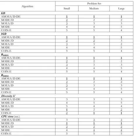
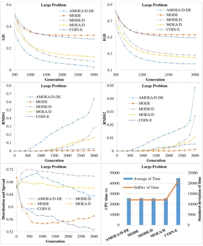
To assess the performance of various algorithms in solving the MaCSP2SAL in Pareto sense, five groups of performance measurements suggested by Jiang, et al. [59] and Chutima and Olarnviwatchai [7] are used in this paper. Obviously, a good algorithm should create various POSs, most of which are located on the approximated true PF. In addition, it would be even better if these POSs are distributed uniformly along the approximated true PF. Since the true PF of the MaCSP2SAL is unknown, the approximated true PF is derived from combining all POSs of all algorithms and applying non-dominated sorting on them. The resultant first PF is an approximated true PF.

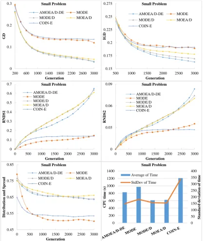
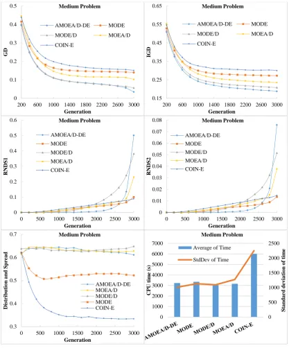
(a) Convergence metric: This metric computes the generational distance of algorithm 𝑗 (𝐺𝐷) which is the least distance between the obtained POSs and the POSs on the approximated true PF. It indicates the proximity level between the non-dominated solutions of algorithm 𝑗 and those in the approximated true PF. If this metric is close to zero, the PF of algorithm 𝑗 is close to the approximated true PF. The formulation of 𝐺𝐷 is as follows.

𝐺𝐷(𝑆𝑗, 𝑆∗) =_|𝑆1

𝑗|∑ min{𝑑𝑥𝑦|𝑦 ∈ 𝑆

∗_}

𝑥∈𝑆𝑗 (33)

𝑑_𝑥𝑦= √∑ (𝑓𝑘(𝑥)−𝑓𝑘(𝑦)

𝑓_𝑘max_−𝑓

𝑘min )

2 𝐾

𝑘=1 (34)

where

𝐺𝐷_𝑗 generational distance of algorithm 𝑗

𝑆𝑗 non-dominated solutions on the first PF of algorithm 𝑗

𝑆∗ _{non-dominated solutions on the approximated true PF}

|𝑆𝑗| number of non-dominated solutions on the first PF of algorithm 𝑗 |𝑆∗_{| number ofnon-dominated solutions on the approximated true PF}

𝑑_𝑥𝑦 Euclidean distance between the obtained solution (𝑥) and solution (𝑦) on the approximated true PF

𝑓_𝑘max _{maximum value of the objective 𝑘 of non-dominated solutions on the approximated true PF}

𝑓_𝑘min _{minimum value of the objective 𝑘 of non-dominated solutions on the approximated true PF}

𝑓_𝑘(𝑥) value of objective 𝑘 of the obtained solution (𝑥)

𝑓_𝑘(𝑦) value of objective 𝑘 of the solution (𝑦) on the approximated true PF

𝑥 obtained solution

𝑦 solution on the approximated true PF

(b) Convergence and diversity metric: This metric indicates both the convergence and diversity of the first PF of the algorithm on a single scale. It computes the inverted generational distance of algorithm 𝑗 (𝐼𝐺𝐷) which is the Euclidian distance between the non-dominated solutions on the first PF of algorithm 𝑗 and the non-dominated solutions on the approximated true PF. If this metric is close to zero, the non-dominated solutions of the algorithm 𝑗 are not only converged to the approximated true PF but also they are diverse. The formulation of 𝐼𝐺𝐷 is as follows.

𝐼𝐺𝐷(𝑆∗_{, 𝑆}

𝑗) =_|𝑆1∗_|∑𝑦∈𝑆∗min{𝑑𝑥𝑦|𝑥 ∈ 𝑆𝑗} (35)

(c) Capacity metric: This metric computes the ratio between the non-dominated solutions on the first PF of algorithm 𝑗 which are on the approximated true PF and its owned non-dominated solutions on the first PF (𝑅𝑁𝐷𝑆1), or between the non-dominated solutions on the first PF of algorithm 𝑗 which are on the

approximated true PF and the non-dominated solutions on the approximated true PF (𝑅𝑁𝐷𝑆2). The

higher the value of 𝑅𝑁𝐷𝑆1 or 𝑅𝑁𝐷𝑆2 is the better algorithm. The formulations of 𝑅𝑁𝐷𝑆1 and 𝑅𝑁𝐷𝑆2 are

𝑅_{𝑁𝐷𝑆1}(𝑆_𝑗) =|𝑆𝑗−{𝑥∈𝑆𝑗|∃𝑦∈𝑆∗:𝑦≺𝑥}|

|𝑆𝑗| (36)

𝑅_{𝑁𝐷𝑆2}(𝑆_𝑗) =|𝑆𝑗−{𝑥∈𝑆𝑗|∃𝑦∈𝑆∗:𝑦≺𝑥}|

|𝑆∗_| (37)

(d) Diversity metric: This metric indicates both the distribution and spread of non-dominated solutions on the first PF of algorithm 𝑗 simultaneously. The good algorithm should have non-dominated solution distributed uniformly and covered all the extreme points of the approximated true PF. The formulation of the diversity metric is as follows. (Note: the lower the value of this metric the better algorithm)

∆∗_(𝑆

𝑗, 𝑆∗) =

∑𝐶𝑐=1𝑑(𝐸𝑐)+∑|𝑆𝑗|_𝑖=1|𝑑(𝑥𝑖)−𝑑̅|

∑𝐶𝑐=1𝑑(𝐸𝑐)+|𝑆𝑗|𝑑̅ (38)

𝑑(𝑥_𝑖) = min

𝑦∈𝑆𝑗√∑ (

𝑓𝑘(𝑥𝑖)−𝑓𝑘(𝑥𝑦)

𝑓_𝑘max_−𝑓

𝑘min )

2 𝐾

𝑘=1 (39)

where

𝑑(𝑥_𝑖) Euclidean distance between consecutive non-dominated solutions

𝑑̅ average of 𝑑(𝑥_𝑖)

𝑑(𝐸_𝑐) Euclidean distance from the non-dominated solutions of the algorithm to the extreme solutions of the approximated true PF.

𝐶 number of extreme solutions

(e) Computational time metric: This metric indicates the CPU time spent by the algorithm until the final solution is reached. A good algorithm should be able to search for a good solution by using less CPU time.

5.

Experimental Design

5.1. Problem Sets

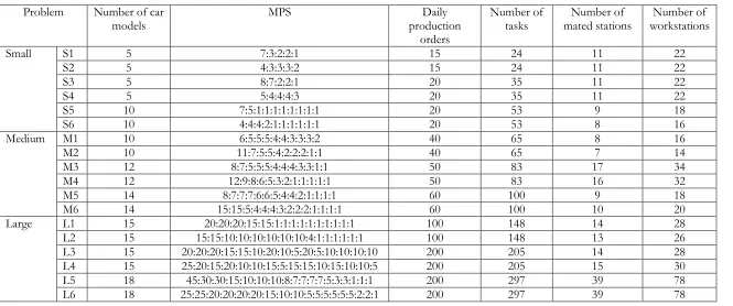
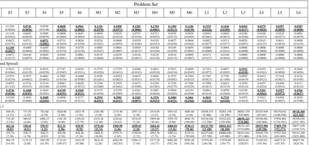
In order to evaluate the effectiveness of AMOEA/D-DE against its competitor algorithms on various production situations, 18 testbed MaCSP2SAL problems with various characteristics are employed (Table 1). The problems are grouped into three different sizes, i.e. small (S1-S6), medium (M1-M6) and large (L1-L6). The sizes of the problems are classified based on the daily number of cars to be produced which is ranged from 15-200. In each problem size, different production requirements are used including a) order-related requirements (i.e. number of car models, MPS, daily production orders), b) car-related requirements (i.e. number of options, number of colours, 𝐶𝐵𝑆_𝑚𝑎𝑥), and c) production-related requirements (i.e. ratio constraints, number of parts, number of tasks in the precedence diagram, number of mated stations and number of stations).

Table 1. Testbed problems.

Problem Number of car

models MPS production Daily

orders

Number of

tasks mated stations Number of workstations Number of

Small S1 5 7:3:2:2:1 15 24 11 22

S2 5 4:3:3:3:2 15 24 11 22

S3 5 8:7:2:2:1 20 35 11 22

S4 5 5:4:4:4:3 20 35 11 22

S5 10 7:5:1:1:1:1:1:1:1:1 20 53 9 18

S6 10 4:4:4:2:1:1:1:1:1:1 20 53 8 16

Medium M1 10 6:5:5:5:4:4:3:3:3:2 40 65 8 16

M2 10 11:7:5:5:4:2:2:2:1:1 40 65 7 14

M3 12 8:7:5:5:5:4:4:4:3:3:1:1 50 83 17 34

M4 12 12:9:8:6:5:3:2:1:1:1:1:1 50 83 16 32

M5 14 8:7:7:7:6:6:5:4:4:2:1:1:1:1 60 100 9 18

M6 14 15:15:5:4:4:4:3:2:2:2:1:1:1:1 60 100 10 20

Large L1 15 20:20:20:15:15:1:1:1:1:1:1:1:1:1:1 100 148 14 28

L2 15 15:15:10:10:10:10:10:10:4:1:1:1:1:1:1 100 148 13 26

L3 15 20:20:20:15:15:10:20:10:5:20:5:10:10:10:10 200 205 14 28

L4 15 25:20:15:20:10:10:15:5:15:15:10:15:10:10:5 200 205 15 30

L5 18 45:30:30:15:10:10:10:8:7:7:7:7:5:3:3:1:1:1 200 297 39 78

Table 1. Testbed problems (Continue).

Problem Number

of options 𝑅𝐶 Constraint (𝑝/𝑞) of colours Number 𝐶𝐵𝑆𝑚𝑎𝑥 Number of parts Possible number of solutions

Small S1 4 1/1,1/2,2/5,1/2 5 3 10 1.08E+07

S2 4 1/1,1/2,2/5,1/2 5 3 10 1.26E+08

S3 4 1/3,1/2,1/3,1/2 5 3 10 2.99E+09

S4 4 1/3,1/2,1/3,1/2 5 3 10 2.44E+11

S5 7 2/5,5/9,10/13,1/2,1/2,1/2,2/3 9 4 20 4.02E+12

S6 7 2/5,5/8,2/3,1/2,1/2,1/2,1/2 9 4 20 8.80E+13

Medium M1 7 1/3,1/2,1/5,5/9,1/4,1/2,5/8 10 4 30 2.64E+33

M2 7 1/3,1/2,1/6,5/9,2/9,1/2,2/3 10 4 30 1.47E+30

M3 8 1/3,1/2,5/12,1/2,2/3,5/11,1/3,5/9 10 4 30 1.74E+44

M4 8 1/3,1/2,5/12,1/2,2/3,5/11,1/3,5/9 10 4 30 4.19E+39

M5 10 10/19,10/21,1/6,5/14,2/3,1/2,10/17,10/17,2/5,10/13 12 5 45 2.25E+55

M6 10 5/8,5/8,1/5,5/9,2/3,5/13,5/7,5/7,10/21,10/11 12 5 45 6.11E+49

Large L1 10 2/3,10/21,5/7,5/11,2/9,2/3,5/6,1/2,5/9,1/5 15 7 60 3.79E+78

L2 10 5/9,2/5,10/21,5/14,2/9,2/3,2/3,1/2,2/7,1/2 15 7 60 9.96E+92

L3 12 5/9,10/13,1/4,1/2,2/5,1/2,5/12,1/2,5/16,5/11,1/2,10/21 15 7 60 >1.00E+100

L4 12 1/2,5/7,1/3,1/2,2/5,1/2,5/12,1/2,10/13,10/21,1/2,10/19 15 7 60 >1.00E+100

L5 12 5/22,5/13,10/33,5/7,1/12,1/3,5/7,5/8,5/8,10/19,5/16,5/9 18 9 75 >1.00E+100