A Multivariate Adaptive Regression Spline Approach for Prediction of Maximum Shear Modulus and Minimum Damping Ratio

Article

A Multivariate Adaptive Regression Spline Approach

for Prediction of Maximum Shear Modulus (

G

max

) and

Minimum Damping Ratio (



_min

)

Pijush Samui

_{* and Dwarkadas Pralhaddas Kothari}

1 Centre for Disaster Mitigation and Management, VIT University, Vellore-632014, India 2 Raisoni Group Of Institutions, Nagpur, India

* E-mail: [email protected]

Abstract. This study uses Multivariate Adaptive Regression Spline (MARS) for determination Maximum Shear Modulus (Gmax) and Minimum Damping Ratio (ξmin) of

synthetic reinforced soil. MARS employs confining pressure (, psi), rubber (r, %) and sand (s, %) as input variables. The output of the MARS is Gmax and min. The developed

MARS gives equations for determination of Gmax and min. The results of MARS have been

compared with the adaptive neuro-fuzzy inference system (ANFIS), multi-layer perceptron (MLP) and multiple regression analysis method (MRM). A sensitivity analysis has been also carried out to determine the effect of each input variable on Gmax and min. This study

shows that the developed MARS is a robust model for prediction of Gmax and min.

Keywords: Maximum shear modulus, minimum damping ratio, multivariate adaptive regression spline, prediction, adaptive neuro-fuzzy inference system, multi-layer perceptron.

ENGINEERING JOURNAL Volume 16 Issue 5 Received 27 March 2012

1.

Introduction

Geotechnical engineers use synthetic reinforced soil for different purposes such as pavement structures, canal lining, erosion control, slope stabilization, piles, walls, liquefaction, etc [1-5]. So, the determination of different dynamic properties {Maximum Shear Modulus (Gmax) and Minimum Damping Ratio (ξmin)} of

synthetic reinforced soil is an imperative task in geotechnical earthquake engineering. Laboratory determination of dynamic properties is a tedious and time consuming task [6]. Recently, Akbulut et al. [6] successfully used Adaptive Neuro-Fuzzy Inference (ANFIS) for determination of Gmax and ξmin of synthetic

reinforced soil. However, the developed ANFIS has low generalization capability. It also did not give equations for determination of Gmax and min.

This article adopts an alternative method based on Multivariate Adaptive Regression Spline (MARS) for determination of Gmax and ξmin of synthetic reinforced soil. MARS is a non-parametric adaptive regression

procedure [7]. It can be considered as a generalisation of classification and regression trees (CART) [8]. It uses a lot of piecewise regression equations in the model. It has been successfully used for solving different problems in engineering [9-16]. This article uses the database collected by [6]. The results of MARS have been compared with the models developed by [6]. This study gives equations for prediction of Gmax and ξmin

of synthetic reinforced soil. This paper is structured as follows: Section 2 describes the MARS model; Section 3 discusses the main results; finally Section 4 contains the conclusion of the paper.

2.

Details of MARS

MARS divides the whole space of input variable into various sub-regions. It defines a different mathematical equation for each area. This equation relates each sub-region of input variable to the output variable. MARS uses the following two-sided truncated power functions as spline basis functions [17].





























otherwise

,

0

t

x

if

,

q

t

x

t

x





























otherwise

,

0

t

x

if

,

q

x

t

t

x

where q is the power and t is knot.

The final MARS model has the following form:

 









m

B

x

a

a

x

f

y

)

(

ˆ

ˆ

where y is the output variable, x is the input variable, a0 is the coefficient of the constant term, M is the number of spline functions, and Bmand am is the m

th

spline function and its coefficient [7] respectively. Confining pressure (, psi), rubber (r, %) and sand (s, %) have used as input of the MARS. The output of the MARS is Gmax and min. So,

x







,

r

,

s



y





G

,





MARS uses the following two steps:

Forward Algorithm: Basis functions are introduced to define Eq. (3). Many basis functions are added in Eq. (3) to get better performance. The developed MARS can show overfitting problem due to large number of basis functions.

 

 

y f x

N GCV C B N   _           



where N is the number of data and C(B) is a complexity penalty that increases with the number of basis

function (BF) in the model and which is defined as:

  

B

B



dB

C





1



where d is a penalty for each BF included into the model and B is number of basis functions in Eq. (3). The

details about d are given by [7].

3.

Details of Present Analysis

This article employs the above MARS for prediction of Gmax and min. The same training and testing dataset

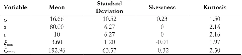
have been used as used by [6]. The data is normalized between 0 and one. Table 1 shows the different statistical parameters of the dataset.

Table 1. Statistical parameter of the dataset.

Variable Mean _Deviation Standard Skewness Kurtosis

 16.66 10.52 0.23 1.50

s 80.00 6.27 0 2.16

r 10 6.27 0 2.16

min 3.60 1.20 -0.01 1.97

Gmax 192.96 63.57 -0.32 2.50

A sensitivity analysis has been done to extract the cause and effect relationship between the inputs and outputs of the MARS model. The basic idea is that each input of the model is offset slightly and the corresponding change in the output is reported. The procedure has been taken from the work of [19]. According to [19], the sensitivity (S) of each input parameter has been calculated by the following formula:

100

j

N

1

j

%

change

in

input

ouput

in

change

%

N

1

S(%)





















where N is the number of data points. The analysis has been carried out on the trained model by varying each of input parameter, one at a time, at a constant rate of 30%. The program of MARS has been constructed by using MATLAB.

4.

Results and Discussion

The performance of the developed MARS has been accessed in terms of Coefficient of Determination (R2_).

Constructive phase: 1.Input:,r, and s 2.Output: Gmax and

min

3.Number of basis function

Pruning phase: 1.Determination of GCV 2. Delete redundant basis function

1.Final MARS model

2. Check testing performance

Check if R closer to 1

Yes

End Change

number of basis functions

No

Fig 1. Flow chart of the MARS model.

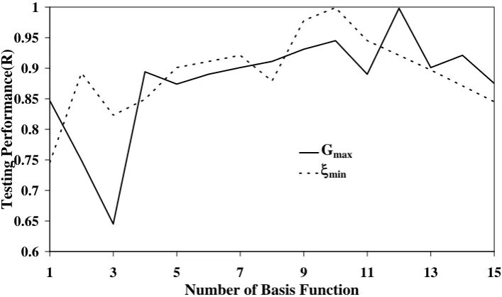
Figure 2 depicts the effect of number of basis function on the testing performance. It is observed from Fig. 2 that 12 basis functions give best performance for prediction of Gmax.

0.6 0.65 0.7 0.75 0.8 0.85 0.9 0.95 1

1 3 5 7 9 11 13 15

Number of Basis Function

Testing

Performance(R) Gmax

min

Fig 2. Effect of number basis function on the testing performance

.

So, 12 basis functions have been introduced in forward algorithm. However, 5 basis functions have been deleted in backward algorithm. So, the final MARS model includes 7 basis functions. The expression of the final MARS model is given below (by putting y=Gmax, a0=0.174 and M=7 in Eq. (3)):

 









1 max

0

.

174

m

m

m

B

x

a

G

Table 2. Basis functions and their corresponding coefficient (am) for Gmax.

Basis Functions Equation Coefficient (am)

B1(x)

max



0

,

r



0

.

0343



B2(x)

max



0

,

0

.

0343



r



B3(x)

max



0

,

0

.

059







B4(x)

max



0

,

s



0

.

545



B5(x)

max



0

,

0

.

545



s



B6(x)

B

 

x



max



0

,

0

.

545



s



B7(x)

max



0

,





0

.

059



*

max



0

,

s



0

.

245



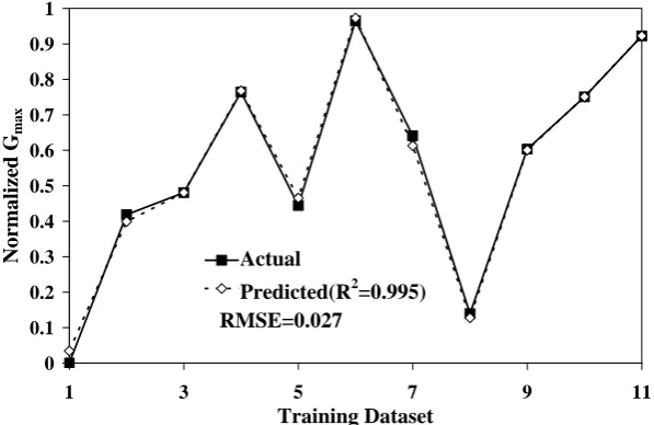
The above Eq. (7) has been adopted for determination of the performance of training and testing dataset. Figure 3 illustrates the performance of the training dataset. As far as the MARS model training is concerned, the developed MARS has successfully captured the input and output relationship. The performance of testing dataset has been shown in Fig. 4.

0 0.1 0.2 0.3 0.4 0.5 0.6 0.7 0.8 0.9 1

1 3 5 7 9 11

Training Dataset

Normalized G

m

ax

Actual

Predicted(R2=0.995) RMSE=0.027

Fig. 3. Performance of the training dataset for Gmax.

0 0.1 0.2 0.3 0.4 0.5 0.6 0.7 0.8 0.9 1

1 3 5 7 9

Testing Dataset

Normalized G

m

ax

Actual

Predicted(R2=0.998)

RMSE=0.024

It is observed from Figs. 3 and 4 that the value of R2 _{is close to one. Therefore, the developed MARS}

shows good predictive ability for prediction of Gmax.

It is clear from Fig. 2 that 10 basis functions give best performance for prediction of min. So, 10 basis functions have been introduced in forward algorithm. However, the final MARS model contains 6 basis functions. So, 4 basis functions have been deleted in backward algorithm. The expression of the final MARS model is given below (by putting y=min, a0=0.189 and M=6 in Eq. (3)): Table 3 summarizes the expression

of Bm and corresponding coefficients (am).

 









1 min

0

.

189

m m

m

B

x

a



Table 3. Basis functions and their corresponding coefficient (am) formin.

Basis Functions Equation Coefficient(am)

B1(x)

max



0

,

r



0

.

0343



B2(x)

max



0

,

0

.

059







B3(x)

max



0

,

s



0

.

545



B4(x)

max



0

,

0

.

545



s



B5(x)

B

 

x

*

max



0

,





0

.

283



B6(x)

max



0

,





0

.

059



*

max



0

,

s



0

.

245



The performance of training and testing dataset has been determined by using Eq. (8). Figures 5 and 6 depict the performance of training and testing dataset respectively. It is clear from Figs. 5 and 6 that the value of R2 _{is close to one. Therefore, the developed MARS has ability for predicting} _min.

0 0.1 0.2 0.3 0.4 0.5 0.6 0.7 0.8 0.9 1

1 3 5 7 9 11

Training Dataset

Normalized

min

Actual

Predicted(R2=0.995) RMSE=0.031

0 0.1 0.2 0.3 0.4 0.5 0.6 0.7 0.8 0.9 1

1 3 5 7 9

Testing Dataset

Normalized G

m

ax

Actual

Predicted(R2=0.998) RMSE=0.024

Fig. 6. Performance of the testing dataset for min.

The results of MARS have been compared with ANFIS, multi-layer perceptron (MLP) and multiple regression analysis method (MRM) developed by [6]. The comparison has been carried out in terms of R2

Figure 7 illustrates the bar chart of R2 _{values of the different model.}

Fig. 7. Bar chart of R2 _{for the different models.}

The value of R2 _{of ANFIS, MLP and MRM is given by [6]. It is observed from Fig. 7 that the}

performance of MARS and ANFIS is almost same. However, the developed MARS outperforms the MLP and MRM models. The developed MARS gives Eq. (6) and (7) for prediction of Gmax and min. But, the

developed ANFIS and MLP did not give any equation for prediction of Gmax andmin.

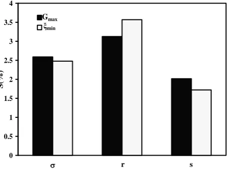
Figure 8 shows the results of sensitivity analysis. It is clear from Fig. 8 that r has maximum effect on

Gmax and min.

0 0.1 0.2 0.3 0.4 0.5 0.6 0.7 0.8 0.9 1

R

2

Gmax min

Fig 8. Sensitivity analysis of the input parameters.

5.

Conclusion

This article successfully adopted MARS for prediction of Gmax and min of synthetic reinforced soil. The

developed MARS has shown good predictive abilities. The performance of MARS is comparable to ANFIS. However, the developed MARS outperforms the MLP and MRM models. Geotechnical engineers can use the developed equations for determining Gmax and min. Sensitivity analysis shows that r has maximum

impact on Gmax and min. This study shows that MARS can be used as a robust tool for solving different

problems in geotechnical earthquake engineering.

References

[1] A. McGown, K. Z. Andrawes, and M. M. Al-Hasani,. “Effect of inclusion properties on the behavior of a sand,” Geotechnique, vol. 28, no. 3, pp. 237-346, 1978.

[2] N. C. Consoli, P. D. M. Prietto, and L. A. Ulbrich, “The behavior of a fiber-reinforced cemented soil,”

Ground Improv, vol. 3, pp. 21-30, 1999.

[3] A. J. Puppala and C. Musenda, ”Effects of fiber reinforcement on strength and volume change in expansive soils,” Transport Res Rec, vol. 1736, pp. 134-40, 2000.

[4] J. J. Murray, J. D. Frost, and Y. Wang, “Behavior of a sandy silt reinforced with discontinuous recycled fiber inclusions,” Transport Res Rec, vol. 1714, pp. 9-17, 2000.

[5] R. L. Santoni, J. S. Tingle, and S. Webster, “Engineering properties of sand–fiber mixtures for road construction,”

Journal of Geotechnical and Geoenvironmental Engineering

in reinforced sands using adaptive neuro-fuzzy inference system,” Soil Dynam Earthquake Eng, vol. 24, pp. 805–814, 2004.

[7] J. H. Friedman, “Multivariate adaptive regression splines,” The Annals of Statistics, vol. 19, pp. 1–14, 1991.

[8] T. Hastie, R. Tibshirani, and J. H. Friedman, The Elements of Statistical Learning. New York: Springer-Verlag, 2003.

[9] P. A. W. Lewis and J. G. Stevens, “Nonlinear modeling of time series using multivariate adaptive regression splines (mars),” Journal of the American Statistical Association, vol. 86, no. 416, pp. 864-877, 1991. [10] T. Ekman and G. Kubin, “Nonlinear prediction of mobile radio channels: measurements and mars

model designs,” in Proceedings of IEEE International Conference on Acoustics, Speech, Signal Processing, 1999, vol. 5, pp. 2667–2670.

[11] C. C. Yang, S. O. Prasher, R. Lacroix, and S. H. Kim, “Application of multivariate adaptive regression splines (mars) to simulate soil temperature,” Transactions of the ASAE, vol. 47, no. 3, pp. 881–887, 2004.

 r s

0 0.5 1 1.5 2 2.5 3 3.5 4

S(%)

Gmax

[12] S. Crino and D. E. Brown, “Global optimization with multivariate adaptive regression splines,” IEEE Transactions on Systems, Man, and Cybernetics, Part B: Cybernetics, vol. 37, no. 2, pp. 333–340, 2007.

[13] E. Deconinck, D. Coomans, and V. Y. Heyden, “Exploration of linear modelling techniques and their combination with multivariate adaptive regression splines to predict gastro-intestinal absorption of drugs,” Journal of Pharmaceutical and Biomedical Analysis, vol. 43, pp. 119–130, 2007.

[14] N. O. Attoh-Okine, K. Cooger, and S. Mensah, “Multivariate adaptive regression (MARS) and hinged hyperplanes (HHP) for doweled pavement performance modeling,” Construction and Building Materials, vol. 23, no. 9, pp. 3020-3023, 2009.

[15] J. D. Andrés, P. Lorca, F. J. D. C. Juez, and F. S. Lasheras, “Bankruptcy forecasting: A hybrid approach using Fuzzy c-means clustering and Multivariate Adaptive Regression Splines (MARS),” Expert Systems with Applications, vol. 38, pp. 1866-1875, 2011.

[16] F. Vidoli, “Evaluating the water sector in Italy through a two stage method using the conditional robust nonparametric frontier and multivariate adaptive regression splines,” European Journal of Operational Research, vol. 212, pp. 583-595, 2011.

[17] S. Sekulic and B. R. Kowalski, “MARS: A tutorial,” J. Chemom., vol. 6, pp. 199–216, 1992.

[18] P. Craven and G. Wahba, “Smoothing noisy data with spline functions: estimating the correct degree of smoothing by the method of generalized cross-validation,” Numer Math, vol. 31, pp. 317-403, 1979. [19] S. Y. Liong, W. H. Lim, and G. N. Paudyal, “River stage forecasting in Bangladesh: neural network