radial basis function network
.
White Rose Research Online URL for this paper:
http://eprints.whiterose.ac.uk/941/
Article:
Bors, A G orcid.org/0000-0001-7838-0021 and Pitas, I (1999) Object classification in 3-D
images using alpha-trimmed mean radial basis function network. IEEE Transactions on
Image Processing. pp. 1744-1756. ISSN 1057-7149
https://doi.org/10.1109/83.806620
[email protected] https://eprints.whiterose.ac.uk/
Reuse
Items deposited in White Rose Research Online are protected by copyright, with all rights reserved unless indicated otherwise. They may be downloaded and/or printed for private study, or other acts as permitted by national copyright laws. The publisher or other rights holders may allow further reproduction and re-use of the full text version. This is indicated by the licence information on the White Rose Research Online record for the item.
Takedown
If you consider content in White Rose Research Online to be in breach of UK law, please notify us by
Object Classification in 3-D Images Using
Alpha-Trimmed Mean Radial
Basis Function Network
Adrian G. Bor¸s and Ioannis Pitas, Senior Member, IEEE
Abstract—We propose a pattern classification based approach
for simultaneous three-dimensional (3-D) object modeling and segmentation in image volumes. The 3-D objects are described as a set of overlapping ellipsoids. The segmentation relies on the geometrical model and graylevel statistics. The characteristic parameters of the ellipsoids and of the graylevel statistics are embedded in a radial basis function (RBF) network and they are found by means of unsupervised training. A new robust training algorithm for RBF networks based on-trimmed mean statistics is employed in this study. The extension of the Hough transform algorithm in the 3-D space by employing spherical coordinate system is used for ellipsoidal center estimation. We study the performance of the proposed algorithm and we present results when segmenting a stack of microscopy images.
Index Terms—Alpha-trimmed mean, radial basis function
net-works, 3-D Hough transform.
I. INTRODUCTION
T
HREE-DIMENSIONAL (3-D) modeling and segmen-tation are important tasks in scene processing, under-standing and visualization [1]–[3]. Several approaches have been adopted in this field and in the following we mention only a few of them. A volumetric image can be seen as an array of voxels at the sites of a 3-D lattice. The main approaches in 3-D object identification consist of representing each object either by a global model description or as a set of component elements. The global description of a 3-D object was considered by using the generalized cylinder model [4] or by minimizing an energy function [5], [6]. Modeling 3-D objects by tracking each slice in a stack of images was employed in [7] and [8]. The object is represented as a set of generalized cylinders in [6] and [8] or as a deformable surface model [9]. The 3-D segmentation in [10] employs a 3-D connectivity algorithm, after appropriate thresholding. Mathematical morphology [11] was used in 3-D domain for segmenting pulmonary trees [12] and brain tissue [13]. Various model-based supervised classifiers have been tested in segmenting 3-D brain images in [14], [15]. Each regionManuscript received October 20, 1997; revised March 23, 1999. The associate editor coordinating the review of this manuscript and approving it for publication was Dr. Fabrice Heitz.
A. G. Bor¸s was with the Department of Informatics, University of Thes-saloniki, Thessaloniki 540 06, Greece. He is now with the Department of Computer Science, University of York, York YO10 5DD, U.K. (e-mail: [email protected]).
I. Pitas is with the Department of Informatics, University of Thessaloniki, Thessaloniki 540 06, Greece (e-mail: [email protected]).
Publisher Item Identifier S 1057-7149(99)09347-1.
is associated with a multivariate Gaussian mixture density in [15]. 3-D modeling from range images using self-organizing maps [16] was employed in [17]. Radial basis functions (RBF’s) were used for 3-D iterative image reconstruction from projection data in [18] and in 3-D shape from shading reconstruction [19].
In this study, we employ an unsupervised classification pro-cedure by using an RBF network for modeling the 3-D scene. The RBF network has a two-layer feed-forward topology and has been successfully employed for functional modeling and pattern classification [20]–[22]. In RBF networks, a function is approximated by a mixture of kernels implemented by the hidden units. The RBF approximation capabilities have been extensively studied [22]–[25]. Due to their functional approximation and localization properties, RBF’s were found attractive for use in computer vision and image processing [26], [27]. Gaussian functions, which geometrically model ellipsoids in 3-D, are used as RBF hidden unit activation functions in the approach described in this study. Mixtures of Gaussian functions have been considered for modeling in many scientific fields. In this approach graylevel and shape are jointly modeled with a set of overlapping Gaussian functions. The input space consists of four features, denoting the voxel coordinates and the graylevel. The parameters of the ellipsoids can be estimated using the normalized first- and second-order moments [28]. The calculation of the ellipsoid parameters by using an approach based on moments corresponds to a classical statistical formulation. Their estimation can be performed by means of the -means clustering algorithm or its adaptive implementation represented by the learning vector quantizer (LVQ) algorithm [16].
A classical training algorithm for RBF networks employs the LVQ algorithm for estimating the Gaussian function pa-rameters [29]. Variants of this algorithm have been derived in order to increase its efficiency in modeling data distributions [26], [30]. An algorithm based on median estimation called median radial basis function (MRBF) was proved to provide better data classification when compared to the classical al-gorithm [21]. The classical moment alal-gorithms are sensitive when data are contaminated by noise. In this study we propose a new RBF training algorithm based on the -trimmed mean statistics. This algorithm orders the data samples associated with a basis function and eliminates a certain percentage of those situated at the extremes of the distribution. The remaining data is averaged. The -trimmed mean algorithm
has been proved a good location estimate in the case when data is contaminated with medium and long tailed distributions [31] and has been employed for image filtering [11], [32]. In the approach considered in this study, the number of samples trimmed away from the given distribution depends on the data statistics [33]. The classical RBF and MRBF training algorithms are particular cases of the proposed algorithm. We prove that alpha-trimmed mean RBF algorithm provides unbiased estimates for the ellipses center and this result can be extended for ellipsoids. A trimming algorithm which discards data samples with large Mahalanobis distances from the center is used for covariance matrix estimation [34]. The use of this algorithm for ellipsoid covariance matrix estimation is studied. Experimental results suggest that the proposed algorithm is efficient in estimating parameters of overlapping ellipsoids or when the ellipsoids are embedded in noise.
A study of the similarities among various clustering and energy-minimization algorithms used for image boundary ex-traction is provided in [35]. The Hough transform (HT) has been applied for finding curve parameters in images [28], [36]. In [28], the HT is treated in the context of the Bayesian theory. LVQ or other clustering algorithms have been used to estimate the parameters of lines and curves in the Hough space [26], [38]. In this study we propose a 3-D extension of the HT for estimating RBF centers in correspondence with the alpha-trimmed mean RBF algorithm. Various ellipsoids are gathered together, based on the graylevel and location proximity criteria, in order to model complex objects. The alpha-trimmed mean RBF network output parameters are calculated based on the backpropagation algorithm [20], [22]. After estimating the network parameters corresponding to the 3-D modeling, the network can be used to reconstruct the objects or for segmenting 3-D scenes.
The pattern classification criterion employed in this study is described in Section II. The alpha-trimmed mean RBF algo-rithm is presented in Section III and its application for object modeling in Section IV. Simulation results when applying the proposed algorithm in synthetic object modeling and in 3-D segmentation of a stack of microscopy images are provided in Section V and the conclusions are drawn in Section VI.
II. THE CLASSIFICATION CRITERION
We employ a Bayesian approach for object classification in volumetric images. Let us denote by the object to be identified and by a 3-D image. The object which provides the maximum a posteriori probability among all the possible candidates is given by
(1)
where is the total number of objects to be found in the volumetric image. The a posteriori probability is expressed by means of Bayesian relationship
(2)
where is the probability associated with 3-D scene modeling from the component objects and is the a priori
probability of the object. We decompose these probabilities in a set of components. This corresponds to the fact that a shape can be represented as a combination of several subsets. The relationship (1) becomes
(3)
where one of the components making up the object is denoted as . Each of the component probabilities can be expressed as an energy function
(4)
where is a normalizing constant and is a function depending on the feature vectors associated with the voxels. The a priori probabilities scaled by a constant are taken as weighting factors denoted by . The relationship (3) can be expressed as
(5)
This structure is implemented in an RBF network. RBF’s prop-erties make them suitable to approximate continuous functions with the desired precision [22]–[25]. They are implemented in a two-layer network, where each input represents a feature entry. The hidden-layer unit embeds a Gaussian function
(6)
where denotes the center vector and the covariance matrix. A Gaussian function statistically models a cluster of data and geometrically represents an ellipsoid in 3-D space.
The network output for data vector is denoted by where and is limited to the interval by a sigmoidal function
(7)
Each network output is assigned to an object.
III. ALPHA-TRIMMED MEANRADIALBASISFUNCTIONS
In the previous section, we have expressed the object probabilities as a sum of locally-activated density functions, modeled by Gaussians. Each voxel in the volumetric image is associated to a feature vector consisting of two parts: its coordinates and graylevel, respectively, denoted as . The Gaussian center is composed of , with the former part representing the coordinates of the ellipsoid center in the 3-D image and the latter its characteristic graylevel. The cross-correlation between the features denoting the coor-dinates and the graylevel is set to zero. The covariance matrix associated to the basis function is:
where models the shape and represents a 3 3 matrix in 3-D and is the graylevel variance. Thus, the function (6) can be decomposed in
(9)
where the first expression of the decomposition is associated to the geometry of the object and the second to the graylevel distribution. This model is embedded in an RBF network.
A classical approach in training RBF networks employs the LVQ algorithm [16] for estimating the hidden unit function center [29]. Similar training algorithms for RBF networks have been considered for curve parameter estimation [26] and channel equalization [30]. These algorithms correspond to the classical statistics theory and provide unbiased results if the distributions are Gaussian and nonoverlapping.
The algorithm proposed in this study is based on an unsu-pervised approach, similar to the LVQ. We generate a set of centers at random and the algorithm calculates the Euclidean distance from a data sample to each of them. The closest center to the given data vector is chosen to be updated:
(10)
where is the closest center to the incoming data sample . A robust statistics based algorithm employing the marginal median for Gaussian center estimation and the median of the absolute deviation from the median for width estimation and called median RBF (MRBF) was proposed in [21]. The theoretical analysis has shown that the bias provided by MRBF is smaller than that of the classical LVQ-based RBF algorithm when estimating the parameters of a mixture of overlapping Gaussians. In this study, a new robust statistics based training algorithm which contains the previous two approaches as particular cases is proposed. Data samples assigned to a specific cluster according to (10) are arranged in the order of their values on each dimension independently. Let us denote them in correspondence to their rank as for
where is the total number of data samples assigned to the -th hidden unit. A very general description of many robust statistics algorithms assigns a weight to each data sample with respect to its rank [31], [37], and provides an estimate of the center, as follows:
(11)
where is the weight depending on the ranking of the
respective data sample. If for ,
then the center is computed by averaging. If for
, and for
[image:4.612.326.534.51.233.2]we obtain the marginal median estimator. In other robust statistics algorithms, is replaced by a function which decreases with respect to the distance of the data sample from the central ordered data sample . In this study we
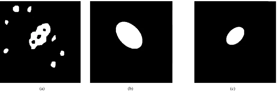
[image:4.612.323.540.262.440.2]Fig. 1. Estimation of the ellipse center after trimming.
Fig. 2. Trimming of an ellipse after ordering its data according to the Mahalanobis distance from the center.
propose to use the -trimmed Mean algorithm [11], [31] which
assigns for , and
for the rest of data samples, where is the percentage of data samples to be trimmed away at each extreme of the th hidden unit data distribution. The -trimmed mean algorithm is a good choice for long and medium tail data distributions and has been extensively used for image filtering [11], [32]. The adaptive implementation of the algorithm updates the parameters of a basis function using only the data samples which are inside of a certain range of ranked samples:
if
otherwise
(12)
where and denote the center estimate and the number of data samples assigned to the th basis function at the moment . We can observe that for we obtain the LVQ algorithm for minimum output variance [39].
(a) (b) (c)
Fig. 3. Estimation of a distorted ellipse. (a) Distorted elliptic shape. (b) Estimating the ellipse using classical moments method. (c) Estimating the ellipse using alpha-trimmed mean RBF algorithm.
length of the data distribution [33]:
(13)
where represent the average of the upper and, respectively, the lower percent of data samples assigned to a specific basis function. The number of data samples to be trimmed away relies directly on the value of
(14)
For long tailed distributions, the amount of data samples to be trimmed is large while for short tailed distributions less samples are trimmed away.
For the second-order statistics, we order the data samples assigned to a basis function according to their Mahalanobis distance from the estimated center , starting with
(15)
After ordering the data samples assigned to the th basis
func-tion according to this measure , the
estimate of the covariance matrix is obtained using ellipsoidal trimming [34]
(16)
where denotes the th ordered data sample according to the Mahalanobis distance (15) and is the trimming percentage in this case. Similarly, with (12) this formula can also be implemented in an adaptive form. The formula (16) corresponds to peeling off observations in shells using a sequence of convex hulls. The formulae (12) and (16) make up the alpha-trimmed mean RBF training algorithm.
IV. OBJECTMODELINGUSINGALPHA-TRIMMEDMEANRBF
In this section we study the application of the alpha-trimmed mean RBF algorithm for estimating the parameters of ellipsoids. The analytic form of an ellipsoid is:
(17)
We can observe that the ellipsoid center and width correspond to the mean and variance of a Gaussian function. The orien-tation of the ellipsoid can be derived from the components of the Gaussian covariance matrix. Algorithms based on first-and second-order moments are used for calculating the ellipse parameters [28] and they can be extended for ellipsoids. However, the classical moment-based method is likely to provide a biased estimate in the case when ellipsoids are overlapping or in the presence of noise.
For simplifying the notation, let us consider an ellipse as the two-dimensional (2-D) case of an ellipsoid. The calculation of the center using (12) is done on each dimension independently and does not depend on the number of entries. The pixels of the ellipse are uniformly distributed in the domain defined by (17). The center of the ellipse is estimated from the normalized first-order moments:
(18)
where denotes the distribution function of the truncated
ellipse and its limits, and denotes
the estimate of the center vector component on the axis. The denominator in (18) calculates the area of the ellipse after truncation. In Fig. 1, the truncation of an ellipse by -trimmed mean algorithm is displayed.
The following proposition has been proved in Appendix A. Proposition 4.1: The center of an ellipse is exactly deter-mined after ordering the corresponding data samples of its distribution and after trimming away an percentage of them at both limits, .
For the ellipse covariance matrix, we calculate the nor-malized second-order moments for the distribution left after trimming, as follows:
Fig. 4. Description of the algorithm for modeling 3-D objects.
where is the function describing the ellipse, trimmed
based on (16), and and
denote the geometrical limits of the ellipse after trimming. The illustration of ellipse trimming by excluding from compu-tation extreme shells of data is displayed in Fig. 2. Evidently, when trimming data samples from an ideal ellipse, a smaller covariance matrix is obtained. The loss of data must be compensated in certain cases. In Appendix B the estimation of the covariance matrix after trimming an ideal ellipse is studied. The conclusion of this study is the following:
Proposition 4.2: The variance of an ellipse after trimming is given by
(20)
where is the th location vector ordered according to the Mahalanobis distance from the center of the ellipse and is the percentage of trimmed data samples associated with the th basis function.
From (15) and (16), we can observe that the estimation of the covariance matrix by trimming does not depend on a specific dimension or on the number of dimensions. The conclusions provided in Proposition 4.1 and Proposition 4.2 for ellipses can be extended for ellipsoids as well.
alpha-trimmed mean RBF algorithm, a distorted elliptic shape is shown in Fig. 3(a). The ellipse estimated by the classical moments method [28] and by the proposed alpha-trimmed mean RBF algorithm are shown in Fig. 3(b) and in Fig. 3(c). It can be observed that alpha-trimmed mean RBF algorithm is robust in estimating the ellipse parameters when data is distorted by noise.
In order to model the geometrical shape by the basis functions we can employ a 3-D extension of the HT in combination with the alpha-trimmed mean RBF algorithm. HT represents a mapping from the image features to sets of points in a parameter space [2], [28], [36]. The parameters provided by the HT have been used as input features for the RBF and LVQ algorithms, in order to detect lines [26] and for texture classification [38]. For voxels where a significant edge is located, we generate a set of parameters which are compatible with the volumetric image features and the hypothesized model. The HT can be used to detect complex parametric curves [28], [36]. However, the number of required parameters increases with respect to the complexity of the model. In order to reduce the computational complexity, HT is employed only for finding estimates of sphere centers to be used in the context of the alpha-trimmed mean RBF algorithm. For finding the object edges we apply a 3-D extension of the Sobel edge detector algorithm which provides both edge intensity and orientation. The transformation from the rectangular to the spherical coordinate system is given by the system of equations:
(21)
(22)
(23)
where are the spherical coordinates corresponding to a voxel in the rectangular coordinate system. After the 3-D Sobel edge calculation, the orientation of the edge with respect to the plane is given by a formula based on (22) and the orientation with respect to axis is derived from (23). We consider a certain volumetric image partition in cubes and we associate an accumulator to each cube. The possible candidates for the centers of the component spheres can be expressed with respect to the locations of significant
edges as
(24)
(25)
(26)
[image:7.612.319.549.56.510.2]for a certain interval . For each from the given interval we increment the accumulator corresponding to all the points as provided by (24)–(26). From (9), we observe that we can train separately the RBF weight components modeling the geometrical shape and the graylevel variance . We use the accumulators provided by 3-D HT as weights in the adaptive alpha-trimmed mean RBF
Fig. 5. Estimating the parameters of the alpha-trimmed mean RBF network.
for estimating centers of spheres:
if
otherwise
(27)
(a) (b)
[image:8.612.44.560.53.309.2](c) (d)
Fig. 6. Modeling a synthetic shape. (a) Original shape. (b) RBF modeling. (c) Alpha-trimmed mean RBF modeling. (d) MRBF modeling.
ellipsoids this produces a function with an elliptic support that is symmetrically distributed with respect to its center. We can observe that the result provided by Proposition 4.1 is valid in this situation as well.
Complex objects in images can be modeled by using shape decomposition based on mathematical morphology [36] or overlapping Gaussian functions [19]. As a consequence of RBF function modeling capabilities [22]–[25], geometrically any continuous object can be represented by a certain number of ellipsoids with a given accuracy. By combining graylevel and geometrical information we can model objects which do not have smooth boundaries. Very irregular objects would require a large number of ellipsoids in order to be modeled. After estimating the hidden-unit parameters according to (27) and (20) we calculate the output parameters . These weights denote the association among the hidden and output units. Positive ’s correspond to ellipsoids which are added in order to model objects and negative ’s correspond to holes (missing parts) in objects. Usually the output weights are estimated based on a priori assumptions [22]. In this study we have applied an unsupervised approach similar to that used for describing moving objects in image sequences [27]. The voxels are assigned to a certain set associated with a hidden unit , after evaluating
(28)
where is provided in (6). In order to group various ellipsoids in distinct objects we employ two criteria: the first criterion considers the geometrical compactness and the sec-ond takes into account the similarity in the graylevel statistics. In the second criterion only the data samples assigned to the neighboring region pairs are considered. The compactness is calculated based on the cardinality between the regions
(a) (b)
[image:8.612.302.557.364.454.2](c) (d)
Fig. 7. Modeling a noisy synthetic shape. (a) Shape corrupted by noise. (b) RBF modeling. (c) Alpha-trimmed mean RBF modeling. (d) MRBF modeling
TABLE I
MODELING ASYNTHETIC3-D SHAPEWHENUSINGLVQ-BASED RBF, MRBF,ANDALPHA-TRIMMEDMEANRBF ALGORITHMS
associated to each two hidden units [40], as follows:
(29)
where and are the sets associated with two hidden units, denotes the cardinal operation and is a 27 voxel neighborhood of the site containing the labels of the respective voxels. This measure calculates the border length between the volumes assigned to two different basis functions [27]. If , then we evaluate the similarity in the graylevel distribution and compare it with a certain threshold. Let us denote by the distribution of the graylevel statistics corresponding to , calculated as a histogram. The similarity is evaluated as the distance between the normalized graylevel distributions associated to the two regions:
If
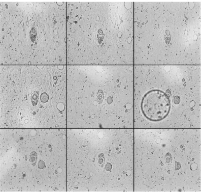
Fig. 8. Frames from a stack of microscopy images representing cross-sections of tooth pulpal blood vessels and surrounding tissue.
where is a threshold and is a decision function for the class which contains the sets . If is small, the 3-D scene will be split in many objects and if it is big, then fewer objects will be considered. are used as target labels for estimating the output parameters. We use the backpropagation algorithm for finding the output parameters [22]
(31)
where is the output provided by the network (7) and is the data target label decided according to (30). The object borders coincide with the classification boundary between their class discriminant functions, as it is provided by the Bayesian classification theory described in Section II. The parameters of the 3-D scene are thus embedded in the network. The hidden units model the characteristics of the ellipsoids and the output units represent objects. The presentation of the 3-D object modeling and segmentation algorithm is shown in Fig. 4. The training algorithm for alpha-trimmed mean RBF algorithm in the context of 3-D object modeling is detailed in Fig. 5.
V. SIMULATION RESULTS
The alpha-trimmed mean RBF algorithm has been tested in many applications. We have used the alpha-trimmed mean RBF algorithm as described in Section III, when modeling a synthetic object. We consider the modeling of a 3-D shape consisting of six spheres of constant intensity with the centers located at
and . The resulting shape is displayed in Fig. 6(a). The coordinates of the voxels composing the shape are considered as inputs in the neural network. After applying (12) and (20), we obtain the parameters describing the given object. Afterwards, the shape is reconstructed from the parameters embedded in the neural network. The modeling results when using RBF, alpha-trimmed mean RBF and MRBF network are displayed in Fig. 6(b)–(d). We distort the shape of the artificial object by adding noise. The noise is uniformly
distributed in the volume and
Fig. 9. Vessel segmentation in the selected frames using classical statistics-based RBF training.
RBF and MRBF algorithm are displayed in Fig. 7(b)–(d). Two measures are considered for numerical comparison. The first error criterion measures the average bias in center location
(32)
where represents the number of spheres and are the original and the estimated location of centers, respectively. A second measure is the volume error and it is calculated as the absolute difference between the volume of the original shape, shown in Fig. 6(a), and the volume representing the object reconstructed based on the estimated parameters, normalized at the size of the original object. The average of the results when applying several times RBF, MRBF and alpha-trimmed mean RBF are provided in Table I. We can observe from this Table as well as from Figs. 6 and 7 that alpha-trimmed mean RBF provides a better result than that of RBF when estimating the original shape from Fig. 6(a), and better modeling capabilities than MRBF when estimating the parameters from the noisy shape. These results show the capability of the proposed algorithm to model a composite shape as well as its robustness to noise corruption.
Fig. 10. Vessel segmentation in the selected frames using alpha-trimmed mean RBF training.
have been assigned with few data samples according to (10) are afterwards discarded. The voxel coordinates weighted by the accumulator cells provided by the 3-D HT and the graylevel are used for modeling the 3-D object shape and structure. The data samples associated with various hidden-units and corresponding to component parts of the objects are organized in data histograms. A segmentation which relies only on the graylevel value would provide spurious patterns all across the image. If the segmentation would rely only on the geometrical shape, the borders of the objects would not be accurately represented or the number of required ellipsoids would be very high. The neighboring 3-D regions which are defined by estimating the hidden-unit parameters, are joined together based on their graylevel similarities. Correspondences among the 3-D regions modeled by the hidden units and the 3-D objects are given by the output weights . After estimating the location, shape and the graylevel parameters, we apply the network on the entire stack of 60 images, on 2 2 pixel blocks. The segmentation of the frames from Fig. 8 using RBF and alpha-trimmed mean RBF is shown in Figs. 9 and 10, respectively. As it can be observed from Fig. 10, the segmentation of the two blood vessels is good and the spurious patterns scattered around the objects are greatly
reduced when using the alpha-trimmed mean RBF algorithm. The 3-D segmentation of the two blood vessels is completely automatic. The alpha-trimmed mean RBF segmentation result is visualized for various perspective angles in Fig. 11(b)–(d).
VI. CONCLUSION
(a) (b)
[image:12.612.68.536.52.549.2](c) (d)
Fig. 11. Three-dimensional representations of microscopy images. (a) Original stack of frames. (b)–(d) Three-dimensional blood vessel segmentation visualized from three different viewing angles.
location, shape and graylevel information of the objects. Each output of the network corresponds to an object.
APPENDIX A
Let us denote the components of the covariance matrix from (17) as
(33)
In order to evaluate the limits of integration in (18) we calculate the tangents at the ellipse parallel with direction,
as follows:
(34)
where denotes the component of and is the vector normal to ellipse and parallel with the axis [28]. After chosing two vectors and
corresponding to the truncated ellipse are:
(35)
The integration limits on the axis are derived with respect to coordinate when considering equality in (17):
(36)
The denominator of the expression (18), representing the area of the truncated ellipse, can be expressed, after changing the variable, and considering as
(37)
Similarly, the numerator from (18) is
(38)
The second integral in (38) is zero and the result of the estimation is
(39)
APPENDIX B
The equation of the ellipse resulted after ordering the data samples assigned to a basis function according to the Mahalanobis distance from the center (15) and trimming a percentage is
(40)
Following a similar derivation as in Appendix A, we obtain the integration limits on axis as follows:
(41)
Similarly, with (36) we derive the integration limits for axis. The area of the ellipse after trimming is
(42)
For one of the covariance matrix components from the numerator in the expression (19) we obtain
(43)
From (42) and (43) we derive the estimate for the variance on axis as follows:
(44)
We obtain similar expressions for the other components of the covariance matrix in the numerator from (19). We observe that for in (44) we obtain the same ellipse width estimate as that provided in the case of the ideal ellipse when using the classical normalized second order moment method [28].
REFERENCES
[1] C. Roux and J.-L. Coatrieux, Contemporary Perspectives in
Three-Dimensional Biomedical Imaging. Amsterdam, The Netherlands: IOS, 1997.
[2] O. Faugeras, Three-Dimensional Computer Vision, A Geometrical
View-point. Cambridge, MA: MIT Press, 1993.
[3] G. Lohman, Volumetric Image Analysis. New York: Wiley-Teubner, 1998.
[4] J. Ponce, D. Chelberg, and W. M. Mann, “Invariant properties of straight homogeneous generalized cylinders and their contours,” IEEE Trans.
Pattern Anal. Machine Intell., vol. 11, pp. 951–966, 1989.
[5] L. D. Cohen and I. Cohen, “Finite-element methods for active contour models and ballons for 2-D and 3-D images,” IEEE Trans. Pattern Anal.
Machine Intell., vol. 15, pp. 1131–1147, 1993.
[6] B. Verdonck et al., “Accurate segmentation of blood vessels from 3D medical images,” in Proc. IEEE Int. Conf. Image Processing, Lausanne, Switzerland, 1996, vol. III, pp. 311–314.
[7] V. Burdin, C. Roux, C. Lef`evre, and E. Stindel, “Modeling and analysis of 3-D elongated shapes with applications to long bone morphometry,”
IEEE Trans. Med. Imag., vol. 15, pp. 79–91, 1996.
[8] Q. Huang and G. C. Stockman, “Generalized stochastic tube model: Tracking 3D blood vessels in MR images,” in Proc. Int. Conf. Pattern
Recognit., Jerusalem, Israel, 1994, pp. 156–160.
[9] C. Davatzikos and R. N. Bryan, “Using a deformable surface model to obtain a shape representation of the cortex,” IEEE Trans. Med. Imag., vol. 15, pp. 785–801, 1996.
[10] M. Joliot and B. M. Mazoyer, “Three-dimensional segmentation and interpolation of magnetic resonance brain images,” IEEE Trans. Med.
Imag., vol. 12, pp. 269–277, 1993.
[11] I. Pitas and A. N. Venetsanopoulos, Nonlinear Digital Filters: Principles
and Applications. Norwell, MA: Kluwer, 1990.
[12] C. Pisupati, L. Wolff, E. Zerhouni, and W. Mitzner, “Segmentation of 3D pulmonary trees using mathematical morphology,” in Proc. Conf.
Mathematical Morphology and Its Applications to Image and Signal Processing, Atlanta, GA, 1996, pp. 409–416.
[13] J. Madrid and N. Ezquerra, “Automatic 3-dimensional segmentation of MR brain tissue using filters by reconstruction,” in Proc. Conf.
Mathematical Morphology and Its Applications to Image and Signal Processing, Atlanta, GA, 1996, pp. 417–424.
[14] M. Kamber et al., “Model-based 3-D segmentation of multiple sclerosis lesions in magnetic resonance brain images,” IEEE Trans. Med. Imag., vol. 14, pp. 442–453, Sept. 1995.
[15] A. Lundervold and G. Storvik, “Segmentation of brain parenchyma and cerebrospinal fluid in multispectral magnetic resonance images,” IEEE
Trans. Med. Imag., vol. 14, pp. 339–349, June 1995.
[16] T. Kohonen, Self Organization and Associative Memory, Berlin, Ger-many: Springer-Verlag, 1988.
[17] S.-W. Chen, G. C. Stockman, and K.-E. Chang, “SO dynamic deforma-tion for building of 3-D models,” IEEE Trans. Neural Networks, vol. 7, pp. 374–387, Mar. 1996.
[18] S. Matej and R. M. Lewitt, “Practical considerations for 3-D image reconstruction using spherically symmetric volume elements,” IEEE
Trans. Med. Imag., vol. 15, pp. 68–78, 1996.
[19] G.-Q. Wei and G. Hirzinger, “Parameteric shape-from-shading by radial basis functions,” IEEE Trans. Pattern Anal. Machine Intell., vol. 19, pp. 353–365, 1997.
[20] A. G. Bor¸s and M. Gabbouj, “Minimal topology for a radial basis functions neural network for pattern classification,” Digital Signal
[21] A. G. Bor¸s and I. Pitas, “Median radial basis function neural network,”
IEEE Trans. Neural Networks, vol. 7, pp. 1351–1364, 1996.
[22] S. Haykin, Neural Networks: A Comprehensive Foundation. Engle-wood Cliffs, NJ: Prentice-Hall, 1994.
[23] E. J. Hartman, J. D. Keeler, and J. M. Kowalski, “Layered neural networks with Gaussian hidden units as universal approximations,”
Neural Comput., vol. 2, pp. 210–215, 1990.
[24] J. Park and J. W. Sandberg, “Universal approximation using radial basis functions network,” Neural Comput., vol. 3, pp. 246–257, 1991. [25] T. Poggio and F. Girosi, “Networks for approximation and learning,”
Proc. IEEE, vol. 78, pp. 1481–1497, Sept. 1990.
[26] L. Xu, A. Krzyzak, and E. Oja, “Rival penalized competitive learning for clustering analysis, RBF net, and curve detection,” IEEE Trans. Neural
Networks, vol. 4, pp. 636–649, July 1993.
[27] A. G. Bor¸s and I. Pitas, “Optical flow estimation and moving object segmentation based on MRBF network,” IEEE Trans. Image Processing, vol. 7, pp. 693–702, May 1998.
[28] R. M. Haralick and L. G. Shapiro, Computer and Robot Vision, vol I. Reading, MA: Addison-Wesley, 1992.
[29] J. Moody and C. Darken, “Fast learning in networks of locally-tuned processing units,” Neural Comput., vol. 1, pp. 281–294, 1989. [30] S. Chen, B. Mulgrew, and P. M. Grant, “A clustering technique for
digital communications channel equalization using radial basis function networks,” IEEE Trans. Neural Networks, vol. 4, pp. 570–579, July 1993.
[31] G. Seber, Multivariate Observations,. New York: Wiley, 1986. [32] S. R. Peterson, Y.-H. Lee, and S. A. Kassam, “Some statistical properties
of Alpha-Trimmed Mean and standard typeM Filters,” IEEE Trans.
Acoust., Speech, Signal Processing, vol. 36, pp. 707–713, 1988.
[33] R. V. Hogg, “Adaptive robust procedures: A partial review and some suggestions for future applications and theory,” J. Amer. Stat. Assoc., vol. 69, pp. 909–923, 1974.
[34] D. M. Titterington, “Estimation of correlation coefficients by ellipsoidal trimming,” Appl. Stat., vol. 27, pp. 227–234, 1978.
[35] A. J. Abrantes and J. S. Marques, “A class of constrained clustering algo-rithms for object boundary extraction,” IEEE Trans. Image Processing, vol. 5, pp. 1507–1521, 1996.
[36] I. Pitas, Digital Image Processing Algorithms. Englewood Cliffs, NJ: Prentice-Hall, 1992.
[37] J.-M. Joliot, P. Meer, and S. Bataouche, “Robust clustering with applications in computer vision,” IEEE Trans. Pattern Anal. Machine
Intell., vol. 13, pp. 791–802, 1991.
[38] A. N. Marana, L. da F. Costa, S. A. Velastin, and R. A. Lotufo, “Oriented texture classification based on self-organizing neural network and Hough transform,” in Proc. Int. Conf. Acoustics, Speech, and Signal Processing, Munich, Germany, Apr. 21–24, 1997, pp. 2773–2775.
[39] E. Yair, K. Zeger, and A. Gersho, “Competitive learning and soft competition for vector quantizer design,” IEEE Trans. Signal Processing, vol. 40, pp. 294–309, Feb. 1992.
[40] I. M. Elfadel and R. W. Picard, “Gibbs random fields, cooccurrences, and texture modeling,” IEEE Trans. Pattern Anal. Machine Intell., vol. 16, pp. 24–37, Jan. 1994.
Adrian G. Bor¸s received the M.S. degree in elec-tronics engineering from the Polytechnic University of Bucharest, Romania, in 1992, and the Ph.D. degree in informatics from the University of Thes-saloniki, Greece, in 1999.
From September 1992 to August 1993, he was a Visiting Research Scientist at the Signal Processing Laboratory, Tampere University of Technology, Fin-land. From 1993 to 1999, he contributed to various European research projects as well as industrial projects while at the University of Thessaloniki. Since March 1999, he has been a Postdoctoral Research Associate, Department of Computer Science, University of York, York, U.K. His research interests include neural networks, computer vision, pattern recognition, and nonlinear digital signal processing.
Ioannis Pitas (SM’94) received the Dipl. Electr. Eng. degree in 1980 and the Ph.D. degree in elec-trical engineering in 1985, both from the University of Thessaloniki, Greece.
From 1980 to 1993, he served as Scientific As-sistant, Lecturer, Assistant Professor, and Asso-ciate Professor in the Department of Informatics, University of Thessaloniki, and has been been a Professor there since 1994. He served as a Visiting Research Associate at the University of Toronto, Ont., Canada, University of Erlangen-Nuernberg, Germany, Tampere University of Technology, Finland and as Visiting As-sistant Professor at the University of Toronto. He was Lecturer in short courses for continuing education. His current interests are in the areas of digital image processing, multidimensional signal processing, and computer vision. He has published over 250 papers and contributed to eight books in his area of interest. He is the co-author of Nonlinear Digital Filters: Principles
and Applications (Boston, MA: Kluwer, 1990) and author of Digital Image Processing Algorithms (Englewood Cliffs, NJ: Prentice-Hall, 1993). He is the
editor of Parallel Algorithms and Architectures for Digital Image Processing,
Computer Vision and Neural Networks (New York: Wiley, 1993).

![[18F]-Fluorodeoxyglucose Uptake in Lymphoid Tissue Serves as a Predictor of Disease Outcome in the Nonhuman Primate Model of Monkeypox Virus Infection](data:image/gif;base64,R0lGODlhAQABAIAAAP///wAAACH5BAEAAAAALAAAAAABAAEAAAICRAEAOw==)