Symmetric Temporal Theorem Proving

(1)

Thesis submitted in accordance with the requirements of the University of Liverpool for the degree of Master in Philosophy

Amir Niknafs Kermani Department of Computer Science

(2)

Introduction

1.1 Introduction

A Symmetric system is a system comprising of some identical processes. These systems contain some identical tasks that are the same for all iden-tical processes. A symmetric system often satisfies a set of properties; for example,safety, meaning ”something bad will not happen”,liveness, mean-ing ”some particular situation must eventually happen” andfairness, mean-ing ”somethmean-ing should happen infinitely often”. There have been numerous attempts to exploit symmetry in systems [15, 34, 30, 16]. However, they mostly involve model checkers. In this thesis we try to tackle symmetry using theorem proving instead.

Automated theorem proving is a collection of techniques to deal with mathematical theorems using a computer program. This technique has been applied into many different logics including temporal logic. Temporal proof is a technique used to ascertain whether a temporal logic formula is valid or not. In this thesis, we consider automated temporal theorem proving, focusing on an extension of the resolution procedure developed by Robin-son [32], namely the clausal resolution method for propositional temporal logic (PTL) [19]. As the complexity of satisfiability for PTL is PSPACE complete, its use becomes more difficult as the considered PTL formulae be-come larger. Our approach is to infer resolution steps in larger problems by considering, and extending, resolution steps in corresponding, but smaller, versions. Based on the steps that have been carried out for smaller formu-lae, we make a ‘guess’ at the steps needed for larger formulae of a similar pattern. Clearly, this will only work if the formulae increase in a regular way and if we have a quick way to validate the ‘guesses’.

(5)

spec-ify these system for arbitary number of processes. One of its sub-fragment known asmonadic FOTL can even be decideable. Unfortunately, even this sub-fragment loses its decidability once equality is added[10]. As an inspira-tion from FOTL, in this thesis, in chapterTemplate we try to explain that if we can prove a symmetric system for i processes, we can greatly reduce the steps required to prove the samesymmetric system withi+ 1 processes. The detail of this has been published inTIME International Symposium on Temporal Representation and Reasoning [28]

The stimulus for this work comes from temporal model checking [7], where the main problem is the state-space explosion that occurs as problems increase in size. In that field, symmetric techniques have been used to tackle larger problems by considering smaller instances. The SPIN model checker [23] method has exploited symmetry to overcome the state-space problems, albeit to a limited extent, and only for certain classes of system. Thus, our aim in this paper is to introduce a symmetric way to increase the efficiency of the resolution method as the size of the problem increases.

After the introductory and preliminary sections, we define symmetric systems. Then we introduce a new notion, thetemplate, which can be used toguess astep resolutionof a large symmetric system from astep resolution of the same system with a smaller number of processes, and finally checking its correctness. By doing this, we can bypass the step resolution for the large system, thus improving the efficiency. We then apply this technique to the deductive temporal verification of acache coherence protocol [11].

For small numbers of identical processes, propositional temporal provers can handle their deductive verification. However, if the number of processes increases, or if the formula is complex, even temporal resolution provers such as TeMP [24] or TSPASS [26] may fail to handle such problems. By applying our technique to such symmetric problems, we can perform automated tem-poral proofs for larger numbers of processes by extrapolating from simpler examples.

(6)

Chapter 2

Preliminaries

2.1 Temporal Logic

Temporal logic is an extension of classical logic, specifically adding operators dealing with time. In addition to operators of classical logic, temporal logic often contains extra operators dealing with time. For example, ’’, meaning always, ’’, meaning in the next moment in time and ’♦’, meaning sometime in the future. These additional operators allow us to construct formalisms such as:

(active process⇒_♦task is done)

Meaning : ”whenever there is an active process, then at some point in the future, our task is achieved.”

Temporal logic was first introduced byArthur Priorand later was further developed byHans Kamp and Amir Pnueli.

2.1.1 Propositional Temporal Logic

Propositional Temporal Logic (PTL)[29] is a logic that isdiscrete,linear and propositional Additionally to classical propositional operator, PTL contains a set of temporal operators that deal with time.

• Discrete: the underlying model of time being isomorphic to the natural numbers, with a distinguished initial point and an infinite future.

• Linear: in each moment in time, there is at most one successor.

• propositional : with no explicit first-order quantification

Basic syntax and semantics

(7)

¬φ At this moment in timeφ is not true φ⇒ψ At this moment in time, ψis true ifφ is true φ⇔ψ At this moment in time, φis true if and only if ψ is true φ∨ψ At this moment in time,φ orψ(or both) are true φ∧ψ At this moment in time, bothφand ψ are true

φ At the next moment in time, φwill be true

φ φis always true (at any moment in time)

♦φ φwill eventually become true

φU ψ φwill be true until ψ becomes true

φW ψ φwill be true unless ψ is true (ψ doesn’t have to become true at all)

In the above table,♦, are unary temporal connectors while U and W are binary temporal connectors. In addition, ”(” and ”)” are used to avoid ambiguity. In later we avoid the use of U and W connectors as one can transform them into a combination of unary connectors.

For the semantics of PTL, let us recall that PTL has a linear and discrete basis that is isomorphic to N, thus the model structure is the following:

M=h_N, πi

whereπ :N7→ P maps each moment in time to the set of propositions ( P

) that aretrue at that moment. Thus, for a structure, M, temporal index (the moment in time),iand a formulaφ we have

hM, iiφ

which is true if, and only if,φis satisfied at the temporal indexiwithin the modelM. For full semantics, let’s look at the following:

hM, ii |=>

hM, ii |=φ iffφis a proposition andφ∈π(i)

hM, ii |=¬φ iffp isnot the case thathM, ii |=φ

hM, ii |=φ∧ψ iffhM, ii |=φand hM, ii |=ψ

hM, ii |=φ∨ψ iffhM, ii |=φorhM, ii |=ψ

hM, ii |=φ⇒ψ iff ifhM, ii |=φthenhM, ii |=ψ

hM, ii |=φ∧ψ iffhM, ii |=φand hM, ii |=ψ

hM, ii |=φ iffhM, i+ 1i |=φ

hM, ii |=φ iff for allj, if (j≥i) and hM, ji |=φ

hM, ii |=♦φ iff there exists j such that(j≥i) thenhM, ji |=φ

hM, ii |=φU ψ iff there existsj≥isuch thathM, ji |=ψ and for allk:i≤k < j,hM, ki |=φ

(8)

2.1.2 Satisfiability, Unsatisfiability and Validity

Given a formulaφ, we sayφis satisfiable if and only if there exists a model

M, which φholds. φisvalid if it holds under all interpretations e.g.

φ⇔true

Finallyφ isunsatisfiable if there is no interpretation thatφ is true.

2.1.3 System Properties

The key motivation for temporal logic has been to specify the dynamic prop-erties for reactive systems. Some of the interesting propprop-erties are safety, meaning ”something bad will not happen”,liveness, meaning ”some partic-ular situation must eventually happen” and fairness, meaning ”something should happen infinitely often”.

Using temporal logic we can specify such properties as follows:

• safety: ¬p

• liveness: ♦p

• fairness: ♦p

2.1.4 First-order temporal logic

First-order temporal logic (FOTL) over the natural numbers is incomplete. Thus there is no finitary inference system1which is sound and complete. Or it could be said that the set of valid formulae of the logic is not recursively enumerable. However, monodic fragments of first-order temporal logic [22], where every subformula can have at most one free variable. In addition, a monodic fragment has a finite inference system. Some of the sub-fragments of monodic FOTL can even be decidable. An interesting sub-fragment of monodic FOTL is monodic monadic where each predicate has, at most, an arity of one. However decidability and completeness only holds for logic without equality. Unfortunately, even this sub-fragment loses its decidability once equality is added [10], thus it is not recursively enumerable.

Syntax of FOTL

Well-formed formulae of FOTL (W F Ff) are generated from the symbols of

PTL together with the following:

• A set, Lp, of predicate symbols represented by strings of lower-case

alphabetic characters.

1

(9)

• A set,L_v, of variable symbols,x,y,z, etc.

• A set,L_c, of constant symbols, a,b,c, etc.

• A set,L_f, of function symbols, f,g,h, etc.

• Quantifiers,∀ and ∃

The set of terms, Lt, is defined as follows.

1. BothLv and Lcare subset ofLt.

2. if t1, . . . , tn are in Lt, and f is a function symbol of arity n, then

f(t1, . . . , tn) is inLt.

The set of well-formed formulae of FOTL(W F Ff) is defined as follows.

1. If t1, . . . , tn are in Lt and P is a predicate symbol of arity n, then

P(t1, . . . , tn) is inW F Ff.

2. if Aand B are inW F Ff, then the following are inW F Ff

¬φ At this moment in timeφis not true

φ⇒ψ At this moment in time, ψis true ifφ is true φ⇔ψ At this moment in time, φis true if and only if ψ is true φ∨ψ At this moment in time,φ orψ(or both) are true φ∧ψ At this moment in time, bothφand ψ are true

φ At the next moment in time, φwill be true

φ φis always true (at any moment in time)

♦φ φwill eventually become true

φU ψ φ will be trueuntil ψ becomes true

φW ψ φwill be true unless ψ is true (ψ doesn’t have to become true at all)

3. IfAis inW F Ff andvis inLt, then∃v.Aand∀v.Aare both inW F Ff.

2.2 Automated theorem proving

(10)

of a logical formula, ϕ, is checked by first negating it and translating ¬ϕ into Conjunctive Normal Form (CNF). Then by using an inference rule, re-peatedly checking for unsatisfiability. If acontradiction is derived, then¬ϕ is unsatisfiable, therefore the original formula isvalid.

2.2.1 Robinson’s Resolution method

Robinson resolution method is a method of theorem proving that proceeds by constructing refutation proofs. It is called proofs by contradiction. This method uses one rule of inference that may have to be applied many times. This approach is particularly suitable for proofs to be done by computers. In this approach, the validity of a logical formula,ϕ, is checked by first negating it and translating ¬ϕ into a particular form, Conjunctive Normal Form (CNF) before applying resolution rules. A CNF form can be represented as:

ϕ=C1∧C2∧C˙n

where eachCi, known as aclause, is a disjunction of literals, and each literal

is either an atomic formula2 or its negation. Typically, this CNF formula is represented as a set of clausesC ={C1, C2, . . . , Cn}.

Having a formula in CNF form, we can apply the resolution rule of inference:

(R1∨p) (R2∨ ¬p) (R1∨R2)

R1 and R2 are disjunctions of literals, and p is a proposition. Since one of p and ¬p must be false, then one of R1 or R2 must be true. Then we can produce a new clause (R1∨R2) that can be added to the set of CNF clauses. We continuously apply the inference rule until an empty clause (false) is generated or no new clause can be generated. If false is derived,

¬ϕ is unsatisfiable, thus the original formulaϕ is valid. This procedure is guaranteed to terminate in propositional logic. The resolution principle also applies to first-order logic formulas in skolemized form. As justification of Robinson’s original statement that resolution provides a “machine oriented” approach, many theorem provers based on resolution have been developed for computers; for example, Otter[27] and Vampire[31] are successful reso-lution based provers.

2.2.2 Temporal Automated Proving

There have been attempts to use Robinson’s resolution technique for Tem-poral Logic. These fall into two main classes: non-clausal and clausal. The

(11)

non-clausal method described in [1] and extended to First-Order Temporal Logic in [2] requires a large number of resolution rules. Although it is un-clear what the maximum number of rules is, having many resolution rules can make implementation problematic, as each rule must be implemented separately, and the decision of which rule should follow is often difficult. On the other hand, a clausal resolution technique was originally introduced in [19] by Michael Fisher. This technique requires the PTL formula to be in a normal form, namely Separated Normal Form (SNF) [18]. This was later refined into Divided Separated Normal Form, which has been found to be particularity useful in developing clausal resolution for FOTL, as it preserve satisfiability of the original formula with only linear growth in size [25].

Separated Normal Form (SNF)

PTL formulae can become complex and difficult to understand. Thus it is useful to replace one complex formula by several simpler formulae which have behaviour equivalent to the original. This transformation process preserves satisfiability and ensures that any model of the transformed formula is a model of the original one.

ThereforeSeparated Normal Form[19] was introduced. In SNF formulae are represented as:

n

^

i=1 Ri

where eachRi, known as a clause, must be of one of the following forms

start⇒

r

_

b=1

lb (an initial rule) g

^

a=1

ka ⇒ r

_

b=1

lb (a step rule) g

^

a=1

ka⇒♦l (a sometime rule)

where eachkb,lb orl is simply a literal.

Divided Separated Normal Form (DSNF)

DSNF is an equivalent alternative to SNF. A temporal problem is comprised of four sets of formulaeI,U,E andS where

(12)

ofI would be of the form:

_

a

la

U: represents the universal part of the problem and contains non-temporal formulae that are universally true. Each element ofU would be of the form:

(_

b

lb)

S: represents the step part of the problem containing step clauses. Each element ofS would be of the form:

(^

c

lc⇒

_

d

ld)

E: represents the sometime part, containing eventualities that must be satisfied infinitely often Each element ofE would be of the form:

♦l

The full temporal problem is characterised by the formula

^

I ∧^U ∧^S ∧^E

where ”V

” means that all elements of subsequent set are conjoined.

As mentioned above, DSNF is particularly useful in developing clausal res-olution for FOTL.

2.2.3 Clausal Temporal Resolution

An overview of the Clausal Temporal Resolution method is as follows:

1. Transform formula A intoSeparate Normal Form (SNF) [17], giving a set of clauses As.

2. Perform step resolution [17] on clauses fromAs until either:

(a) A contradiction is derived, in which case A is unsatisfiable; or

(b) No new resolvent are generated, in which case we continue to step(3).

3. Select an eventuality from withinAs, and performtemporal resolution

(13)

4. If all eventualities have been resolved, then A is satisfiable; otherwise, go back to step (3).

Thesoundness,completenessandterminationof this method was proved in [19]. The basis of the above method is the following two-resolutions rule:

• Step Resolution:

(initial) (R1 ∨p ) (step) (L1 ⇒ (R1∨p))

(R2 ∨ ¬p) (L2 ⇒ (R2∨ ¬p))

(R1 ∨R2) (L1∧L2) ⇒ (R1∨R2))

• Temporal Resolution:

♦l

(L⇒ ¬l) ¬L

While step resolution closely resembles the classical resolution rule, the key inference rule in clausal temporal resolution, namely the temporal resolution itself, requires further steps. The translation to SNF restricts the PTL clauses to be of a certain form.

The formula (L ⇒ ¬l) is called the loop formula and the process must reconstruct this formula. The process of reconstructing the loop for-mula is known as loop search. The conclusion of temporal resolution is a clause that is always true at any moment in time. Such a clause is called universal clause. However, (L ⇒ ¬l) can only be constructed by a combination of universal and step clauses. L is a disjunction of conjunc-tions of literals (i.e. in DNF); therefore, its negation is a conjunction of clauses, which is added to the set of universal clauses. Loop searchwas orig-inally developed by Clare Dixon in [12]. It was further developed in [14], so classical automated reasoning can be used for this purpose.

2.2.4 TSPASS

TSPASS[26] is an implementation of clausal temporal resolution based on the first-order theorem prover SPASS [35]. It implements temporal resolu-tion for monodic first-order temporal logic. TSPASS implements a number of simplifications and enhancements over the clausal temporal resolution approach as follows:

• It uses thesimplified clausal temporal resolution calculus [9].

• It is based on ordered resolution [3].

(14)

TSPASS is currently available and can be found at:

http://lat.inf.tu-dresden.de/~michel/software/tspass/

2.2.5 TeMP

TeMP [24] is another implementation of clausal temporal resolution based formonodic first-order temporal logic. It is based on the first-order theorem proverVampire [31]

TeMP is currently available and can be found at:

http://www.csc.liv.ac.uk/~konev/software/TeMP/

TSPASS and TeMP are usually competitive; sometimes one can perform better than the other on different scenarios and examples, but a combination of both can also be useful.

2.3 Symmetric system

A symmetric system comprises of some identical processes. These systems contain some identical tasks that are the same for all identical processes. Preferably these systems should be specified for arbitrary number of pro-cesses.

The aim is to first specify these systems and then check some of the properties they might have. One way of specifying these systems is to use a temporal logic specification; for instance, we can use PTL to specify a system for i processes, then use a PTL prover to verify and check certain properties.

This procedure works as follows; say φi is a specification of a

symmet-ric system Si with i processes. We also have a property ψi of system Si.

We want to check whether ` φi ⇒ ψi. This can be achieved by proving

that one temporal formula implies another. One way of doing that is by using clausal resolution [19] for PTL, in which we check forunsatisfiablity of

¬(φi⇒ψi). This technique is based on a proof procedure for classical logics

by Robinson[32]. However, as previously mentioned, there might be an un-known number of processes in such systems, therefore, proving¬(φi ⇒ ψi)

can only provide proof for iprocesses and cannot determine the proof for, say,i+ 1 processes.

(15)

with specification and proof of a strict set of symmetric systems for an arbitrary number of processes.

2.4 Parameterised System

A parameterised system is a distributed system comprising of N identical processes. Every process has inner states known as’local state’; e.g. initial and final states. Processes in a parameterised system can interact with each other. This interaction results in some general states known as’global states’ within a system. Cache Coherence Protocol [11, 20] is an example of such a system. Parameterised systems are considered to be symmetric as systems contain of identical processes.

2.4.1 Cache Coherence Protocol

In a shared-memory multiprocessor systemlocal caches are used to reduce memory access latency and network traffic. Although local caches improve system performance they introduce thecache coherence problem as multiple cached copies of the same block of memory must be consistent at any time during a run of the system. A cache coherence protocol ensures the data consistency of the system: the value returned by a read must be always the last value written to that location. cache coherence protocolsare an example of Parameterised systems.

Automatically checking the safety properties independently from the number of processors has been tackled using general purpose, infinite-state symbolic model checking [11]. Alternatively, one may verify cache coherence protocols for all possible dimensions by first translating into monodic first-order temporal specification and then applying temporal theorem proving. This has been done in [20]. The following correctness conditions are the most important for cache coherence protocols:

1. non co-occurrence of state: some specific local states q1 and q2 cannot appear in the same global state.

2. at most one: a local state q can appear at most once - i.e. be the state of no more than one processor - in any global state.

Even thoughcache coherence protocols can be represented as monodic first-order formulae, and then be verified using a first-first-order prover, it is still hard to prove some properties. The reason for this difficulty is the general difficulty of first-order formula.

(16)

we lose expressiveness but on the other hand gain advantage over decidability of the formula.

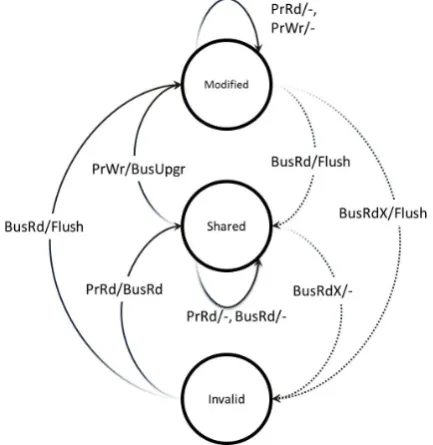
MSI Protocol

The MSI protocol is a basic cache coherence protocol that is used in multi-processor systems.

MSI has three components. Every process can be in exactly one of these components:

• Modified: The block has been modified in the cache. The data in the cache is then inconsistent with the backing store (e.g. memory). A cache with a block in the ”M” state has the responsibility to write the block to the backing store when it is evicted.

• Shared: This block is unmodified and exists in at least one cache. The cache can evict the data without writing it to the backing store.

• Invalid: This block is invalid, and must be fetched from memory or another cache if the block is to be stored in this.

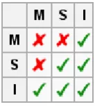
[image:16.595.262.331.458.537.2]

For any given pair of caches, the permitted states of a given cache line are as follows:

Figure 2.1: Relation between two processes in MSI Protocol

As the figure 2.1 shows, two processes cannot be in the Modified state at the same time. Furthermore, if one process is in the Shared state, no other process can be in theModified state.

Figure 2.2 demonstrates this concept in more detail, how each process in MSI can read/write either locally or globally, meaning; reading from the local cache (LR), writing to the local cache (LW), writing to memory (BW) and reading from memory (BR).

If the process is ininvalid state then

(17)

• LW : process has to put a write request on the bus and then move to shared state.

• BR : process doesn’t have to do anything (stays in the same state).

• BW : process doesn’t have to do anything (stays in the same state).

If the process is inshared state then :

• LR : process doesn’t have to do anything (stays in the same state).

• LW : process doesn’t have to do anything (stays in the same state).

• BR : process has to write back to memory then move toshared state

• BW : process has to write back to memory then move toinvalid state.

If the process is inmodified state then:

• LR : process doesn’t have to do anything (stays in the same state).

• LW : put invalidation request on the bus to ask everyone to invalidate their copy then move to modified state.

• BR : process has to write to memory then move toshared state.

(18)

[image:18.595.187.404.324.547.2]

(19)

Chapter 3

Template

In this chapter we describe a formal representation of formulas in a symmet-ric system. This representation shows how we can capture such similarties and eventualy use them in order to improve our proof.

3.1 Definition

Template is a mean to sort and group disjunctions of logic formula from a symmetric system. Typically it is a way of representing a disjunction or a conjunction of propositions. More formally we can define atemplate as :

Definition 1 A template is a set of expressions of the form q or px, (The

latter is just a predicate labelled with x) where p is a state of a symmetric system and x is a variable referrering to the process. If the template does not have a variable it is therefore called constant

In above definition,pis the encoded state of a process as proposition and x is the process number thatp is referring to. For example, p1 is the state p of process 1, where asq because it doesn’t have any variable is therefore aconstant.

The variables in a template is bounded to the total number of identical processes in a specification of a symmetric system.

3.2 Creation

(20)

Algorithm 1

1: proceduretemplateCreation(Formulaφ) 2: t-← ∅

3: for all propositionp inφdo

4: if p is constantthen . ifpdoesn’t end with number 5: t-.add(p,0)

6: else

7: p0 ←stateOf(p) 8: k←processOf(p) 9: if isUsed(k) then

10: v=thecurrentvariablethatisusedf orprocessk 11: t-.add(p0, v)

12: else

13: v=af reshvariable 14: t-.add(p0.v)

15: end if

16: end if

17: end for 18: return t-19: end procedure

An exampleof using Algorithm 1 to create a template as follows: Suppos-edly we a have a disjunctφsuch as

φ=p1∨p2∨q3∨r3∨c

Lets assume these propositions refer to a symmetric system’s states ofp, p, q, r, c and numbers stating their unique process. For simplicity of tracking the re-lation between states and propositions same letters are used for refer to each state and its represntitive proposition. We define a template t- =∅.

Now lets look at the first proposition inφ,p1 is statepbelonging to process 1. since process 1 has yet used in t-, we define a newvariant x1 and addpx1

to t-.

By looking at the next proposition in φ(p2) we can add px2 to t-. qx3 can

be added to t- with the same procedure fromq3. The next proposition is r3. however process 3 has been used in t- before, therefore we are not going to create a new variant and used the variant that this process was referred to. Thus addingrx3 to t-. The last proposition is c. However this is not referred

to any process. Therefore its a constant. so we simply addcto t-. We finally end up with the following for our template.

1_{t- =}_{_p

x1, px2, qx3, rx3, c}

3

1

(21)

.

Definition 2 Template lead is a means to expand a template t to be used for the same system with more processes.

We say template t-0 is a symbolic lead of t- iff

t-0= t-∪q

whereq is:

• q=∅, or

• q is a set of all states in t- that are marked with at most one variable within

t-Algorithm 2 is used to produce all the symbolic lead for a template. In addition to check if a template t-0 is alead of t- we can use Algorithm 3.

Algorithm 2

1: procedureTemplateSymbolicLead(template t) 2: let leadbe a set of Templates.

3: array v← Distinct variables int

4: lead.add(t) . every template is a symbolic lead of itself 5: newV ar← a variable that is not inv

6: for all variantv int do 7: s← variants ofv int 8: q← ∅

9: for all i∈s do

10: q.add(inewvar) . Add variantiwith variable newvar to q

11: end for

12: lead.add(q) 13: end for 14: returnlead 15: end procedure

Algorithm 3

1: procedurecheckTSL(templates t, t0) . check ift0 is a TSL of t 2: let sett00 ← T emplateSymbolicLead(t)

3: for all templatettint00 do 4: if tt==t0 then

5: return true

6: end if

(22)

3.3 Producing clauses from Template

As we can create a template from a formula we can also produce the formula using a template. For example giventemplate:

t- ={px1, px2, rx2, c}

3

we can create the following DNF:

((p1∨p2∨r2∨c)∧(p1∨p3∨r3∨c)∧(p2∨p1∨r1∨c)∧(p2∨p3∨r3∨c)∧(p3∨p1∨r1∨c)∧(p3∨p2∨r2∨c))

Definition 3 Two templates t-,t-0 are equal iff they produce identical clauses regardless of clause orderings fork processes.

In Algorithm 4 it is shown how to create a DNF clauses from atemplate. Let’s consider t- set. We know there are three processes invovled and the set contains four expressions{px1, px2, rx2, c} with two variables {x1, x2} and a

constantc. Algorithm 4 simply create DNF clauses containing #V ariables∗

#P rocesses(2∗3 = 6) disjunctions. since c is a constant, then it will be repeated in every clause. and variables will be replaced by process numbers. For example, if in a clause px1 is replaced by p1 then px2 and rx2 will be

(23)

Algorithm 4

1: procedureclauseFromTemplate(t-,N) . Template T and N processes.

2: mapper ←array of distinct variables

3: F F ← ∅ .A set of conjunctions of formula

4: array A ← {1, . . . , v}

5: changeable←v−1 6: while truedo

7: clause← conjunction of constatns in T 8: fori = 0 to v do

9: for allstat∈T do

10: if stat.variable=mapper[i]then 11: clause←clause∧stateA[i]

12: end if

13: end for

14: end forF F.add(clause) 15: if A[0] =n−v+ 1then

16: return FF . TERMINATE

17: end if

18: if A[changeable] = (N−(v−(changeable+ 1))) then 19: changeable− −

20: end if

21: for i←v−1 downto1 do

22: if A[i]<(N−(v−(i+ 1)))then 23: changeable=i;break;

24: end if

25: end for

26: q←populate(V, A, changeable) 27: A←q

28: end while 29: return F F 30: end procedure

31: procedurepopulate(V, A, changeable) 32: array q

33: fori= 0 to changeable-1do 34: q[i]←A[i]

35: end for

36: q[changeable]←A[changeable] + 1 37: fori←changeable+ 1 toV do

38: q[i]←q[changeable] + (i−changeable) 39: end for

(24)

We now provide an overview of how we use symmetry to remove some of the complexity in temporal resolution refutations for larger instances of a problem. For simplicity of presentation, in what follows we assume that φ contains both the specification of the system and the negation of the property (and thus we are applying temporal resolution toφin an attempt to show unsatisfiability) and thatE ={_♦l}.

1. Instantiate a monodic first-order temporal formulaφto give the PTL formulaφi with a fixedi (initially,i= 1).

2. Run the clausal propositional resolution method onφi.

3. If a contradiction is not derived, increment i and return to step 1 (in this case, the property requires some minimal number of processes before it holds). If a contradiction foriprocesses is derived, move to step 4.

4. From the results gathered from step 2, try to guess a loop set of potential loop formulae for the eventuality♦l in the instance of the specification with a larger number of processesφj (with j > i).

5. If the loop set is empty then incrementiand go to step 1, else continue to step 6.

6. Select a loop formula candidateL from the loop set and check if L is indeed a loop formula in this larger instance of the problem (i.e. φj).

If theloop check procedure returns ’yes’ then go to step 7, otherwise remove Lfrom the loop set and return to step 5.

7. Once it is confirmed thatLis indeed a loop formula, replace the even-tuality rule applied for♦lwith the conculision¬Linφj and run the

temporal theorem prover.

8. If a contradiction is obtained, go to step 1 settingi=j, otherwise go back to step 5.

Thus, if we fail to successfully guess a loop that works for refutations in problems with larger numbers of processes, then we must continue applying the full temporal resolution procedure to successively larger instances of the problem. If we do guess a suitable loop for a larger instance, then we can carry out proof in that instancewithout the necessity of temporal loop search (i.e. with a DSNF problem with emptyE) — this issignificantly faster.

In what follows, we introduce machinery to analyse loop formulae col-lected from a successful run of the theorem prover on φi in step 2 of the

algorithm.

3.4 “Guessing” Loop Formulae

(25)

same behaviour and therefore, give a direction to our guesses. Template is mainly used to “guess” the loops needed for the temporal specification of the system containing more processes.

Given resolvent clauses for ♦l of system φk , we create the templates

of individul disjunct and add them to a set of templates. This procdure is calledgrouping.

Definition 4 A group is the transformation of a template t- to a set of formulaeF

group:template→F

The function to achieve such transformation is called grouping

To group the formulae with the 5 algorithm below, we assume that the give formulae is a resolvent of the loop for a symmetric system.

Algorithm 5

1: procedureGroupFormulae(L) . L is a loop formula in DNF form 2: let F ={l1 ,. . . ,lk}

3: let t- be the template for a li inF

4: let g=∅

5: while F 6=∅do 6: for all f inF do 7: let Q=∅

8: if f can be represented with t-then 9: add f toQand remove f from F

10: end if

11: end for

12: addt7→Qtog

13: let t- be the template for another li inF

14: end while 15: returng 16: end procedure

(26)

Algorithm 6

1: procedureTemplateSymbolicLead(templatet-) 2: let leadbe a set of Templates.

3: array v← Distinct variables in

t-4: lead.add(t-) . every template is a symbolic lead of itself 5: newV ar← a variable that is not inv

6: for all variantv in t- do 7: s← variants ofv in t-8: q← ∅

9: for all i∈s do

10: q.add(inewvar) . Add variantiwith variable newvar to q

11: end for

12: lead.add(q) 13: end for 14: returnlead 15: end procedure

Similar to a loop formula, which can be thought of as a set of conjunc-tions, we define aloop-templateas asetof templates t-1,t-2,. . .,t-k. Intuitively,

a loop template represents all conjunctions of literals from a loop formula. Aloop-template T- is apredecessor of T-0 if, and only if,

• T- and T-0 both contain the same number of templates, and

• for each template t- in T- there is a template t-0 in T-0 such that that t-0 follows from t-.

Theorem 1 Let t-, t-0 be templates and Lbe a loop formula such that for no two conjunctsF, F0 of L we haveF ⊆F0. Then if t-0 follows from t-, the loop formula L cannot contain instances of both t- and t-0, unless t-0 is a syntactic variation of t-.

PROOFLet tand t0 be two templates for loop formula L, since t0 follows from t, then t0 = t∪q if q = Ø then t0 is a syntatic variabtion of t.(1) if q 6= Ø then we have to prove that for every conjunct l1 that is produced fromtfor n number of processes, there is a conjuctl2 that will be produced fromt0 for n in such a way that l1⊆l2 orl2 ⊆l1. 2

This will be sufficient because for every cunjuct F1 and F2 in L we have F1 *F2. Therefore this proves thatL cannot contain both conjuncts from

t and t0 unless (1). Since l2 is a bigger conjunts than l1 because it has at least one more proposition. therefore,

l2⊆l1

2 _number_n_{is greater than the number of distinct varibles of}_t_and_t0

(27)

Based on this result, we first present a naiveGuessedLoopTemplate algo-rithm that enumerates possible loop templates that follow from the current loop template obtained by theGroupFormulae algorithm.

There are two problems with the algorithmGuessedLoopTemplate. First, it can potentially introduce n2 guesses, where n is the maximum number of propositions in a loop formula , which can be too many to prac-tically consider. The second, more serious problem, is that the algorithm only produces templates that follow from the current loop template. In some cases, the loop formula for an instance of the symmetric system for a larger number of processes is not an instance of any template for a smaller number of processes. Therefore, we need more information to produce a loop. The algorithmGuessedLoopTemplate2produces a smaller number of guesses based on loop formulae forLi andLi+1 whereLi is the loop for a

specifica-tion with specificaspecifica-tion withiprocesses andLi+1 is the loop for specification for a specification withi+ 1 processes

Example. Suppose that for an instance of a symmetric systemφithe loop

formula is just a single conjunction of literals. Then the loop template is a singleton {ti}, where ti = {ax, by}. Using GuessedLoopTemplate we obtain the following set of possible loop templatesG forφi+1:

G={{ax, by},{ax, ay, bz},{ax, by, bz}}.

Suppose now that the loop template for φi+1 is ti+1 = {ax, ay, bz}.

Guided by this additional knowledge, the algorithm GuessedLoopTem-plate2, generates a smaller guess forti+2:

G0={{ax, ay, az, bd},{ax, ay, bz}}.

Now, once we have a guess for a loop formula we need to check whether it is indeed a loop or not.

3.5 Checking Loop Guesses

In order to present an algorithm checking whether a given formula is a loop formula, we need to give more detail on how eventuality resolution works. Given a DSNF (I,U,S,E) with E = {_♦l}, the loop formula L should satisfy the following properties (for details see [13]):

1. U ∪ S |=(L⇒ ¬l),

2. U ∪ S |=(L⇒ L).

(28)

Both properties can be checked in a similar manner. To check (2), we form a new DSNF3 (I0,U0,S0,E0) as follows

I0 ={L} S0=S ∪ {¬L} U0₌_U _E0₌_∅

and run temporal resolution on the resulting set of clauses. If a contradiction is derived,L is a loop formula for the original DSNF.

Theorem 2 For a DSNF (I,U,S,E) with E ={_♦l} and a formula L we haveU ∪ S |=(L⇒ L) if, and only if, (I0,U0,S0,E0) is unsatisfiable.

PROOF Loop formuale is created using step and universal clauses thus, the properties of the loop has nothing to do with thestart and eventuality clauses. now let’s assume our system specification is

ϕ=U ∪ S

and our property to check is

(L⇒ L)

by refutation U ∪ S |= (L ⇒ L) is valid iff ϕ∧ ¬((L ⇒ L) is unsatisfiable. Note:

(¬((L⇒ L)⇔_♦(L∧ ¬L))

Another way of writing aneventuality formuale is

♦(L∧ L)⇔((L∧ ¬L)∨ (L∧ ¬L)∨ (L∧ ¬L). . .)

Since the assumption is thatLis the loop formulae thus it is sufficient enough to check for satisfiability of the first portion of the formual that is :

ϕ∧(L∧ ¬L)

Now we can create our DSNF formula to be the set:

I0 ={L} S0=S ∪ {¬L} U0₌_U _E0₌_∅

3

(29)

3.6 Applying the Technique

The algorithms in the previous section have been applied to the verifica-tion of the MSI Protocol [11]. To check the “non-co-occurrence of states” property, we add the negated property:

♦(∃x, y.(S(x)∧M(y)))

to the specification and then run the proof procedure. If the combined for-mula is unsatisfiable, then we know that the “non-co-occurrence” property holds.

It is also worth mentioning that, we are using two different Theorem Provers, namely TSPASS[26] and TeMP [24]. There are two reason for this combinations, one is that based on the specification one can perform better than other one. In addition, since they are used as ’Black Box’ each can produces different set of useful outputs which then can be used for later investigations. To describe the approach in detail, we provide a walk through a run of the algorithms. All the used algorithms have been programmed, however they have not yet put together. Also the decision of what prover to be used is decided by the user. Nevertheless, the automation of each part is relatively easy and is set for our future work. First, we ran the temporal prover TSPASS on an instance of the MSI protocol with two processes. Through the internal processes of TSPASS, the property is transformed into

♦(¬wait for l)

and loop search returns the following loop formulaloop2:

(wait for l ∧i1)∨(wait for l∧i2)∨

(wait for l ∧m1∧m2)∨(wait for l∧s1∧s2).

From this, we can extract the loop template T2 to be:







{wait for l, iX},

{wait for l, mX, mY},

{wait for l, sX, sY}







Now we can use theGuessedLoopTemplatealgorithm to create a set of loop templatesT T to be used forMSI3 and then derive a potential loop formula to be tested using theTestLoop algorithm. Unfortunately, at this stage we are unable to find an appropriate loop forMSI3, and therefore turn to theGuessedLoopTemplate2algorithm. We run TSPASS onMSI3and

2

Time to prove property in MSI protocols without any changes

3

(30)

Number of processes Original Problem2 Modified Problem3 results

2 0.060s 0.011s Unsatisfiable

7 ∞ 35.108s Unsatisfiable

[image:30.595.120.503.126.255.2]

Table 3.1: Performance Comparison using the TeMP [24] Clausal Resolution Prover

extract the looploop3 from it:

(wait for l ∧i1∧i2)

∨ (wait for l ∧i1∧i3)∨ (wait for l ∧i2∧i3)

∨ (wait for l∧m1∧m2∧m3)∨ (wait for l ∧s1∧s2∧s3)

∨ (wait for l ∧s1∧s2∧i3)∨ (wait for l ∧s1∧s3∧i2)

∨ (wait for l ∧s2∧s3∧i1)

∨(wait for l ∧m1∧m2∧i3)

The loop template for the above formulae isT3 (X,Y and Z are variants):

          

{wait for l, iX, iY},

{wait for l, mX, mY, mZ},

{wait for l, sX, sY, sZ}},

{wait for l, mX, mY, iZ},

{wait for l, sX, sY, iZ}

          

At this stage we use T2 and T3 in GuessedLoopTemplate2(T2, T3) to produce a set of template guesses T T4 forMSI4. As before, once we have the templates we produce the formulae and test them. One of the loop formulae candidates extracted from one of the templates in T T4, namely from           

{wait for l, iX, iY},

{wait for l, mX, mY, mZ, mq},

{wait for l, sX, sY, sZ, sq},

{wait for l, mX, mY, mq, iZ},

{wait for l, sX, sY, sq, iZ}

          

(31)

(32)

Chapter 4

Related work

A survey on the use of symmetry in model checking can be found in [34]. Indexed Simplified Computational Tree Logic (ISCTL), introduced in [16], allows one to specify and verify properties of parametrised systems, where the index corresponds to the number of processes. Our research differs in that our main focus is the speed of reasoning rather than representation issues.

Emerson and Kahlon [15] tackle the verification of temporal proper-ties for parametrized model checking problems in an asynchronous systems. They reduced model checking for systems of arbitrary sizen to model check-ing for systems of size (up to ) a small cutoff sizec. Furthermore, in [30], Pnueli, Ruah and Zuck used the standard deductive INV rule for prov-ing invariance properties, to be able to automatically resolve by finite-state (BBD-based) methods with no need of theorem proving. They have devel-oped a system to model check a small instances of the parametrised system in order to derive candidates for invariant assertions. Therefore, their work results in an incomplete but fully automatic sound method for verifying bounded-date parametrized system.

Giorgio Delzanno proposed a method [11] to verify safety properties of parametrized cache coherence protocols using symbolic model checkers for infinite-state based on real arithmetics [21].

In [8], Clarke, Jha and Filkorn investigated techniques for reducing the complexity of temporal logic model. They show how symmetry can be fre-quently used to reduce the size of the state space that must be explored during model checking in finite state systems.

(33)

Chapter 5

Future work

The algorithms presented in this thesis constitute a first step towards prac-tical deductive verification of symmetric systems. While the preliminary re-sults presented in Table 3.6 are encouraging, we clearly need a much greater performance improvement before systems involving a realistically large num-ber of processes can be verified.

(34)

Chapter 6

Conclusion

(35)

Bibliography

[1] Mart´ın Abadi and Zohar Manna. Nonclausal temporal deduction. In Proceedings of the Conference on Logic of Programs, pages 1–15, Lon-don, UK, 1985. Springer-Verlag.

[2] Mart´ın Abadi and Zohar Manna. Nonclausal deduction in first-order temporal logic. J. ACM, 37(2):279–317, 1990.

[3] Leo Bachmair and Harald Ganzinger. Ordered chaining calculi for first-order theories of binary relations, 1995.

[4] Abdelkader Behdenna, Clare Dixon, and Michael Fisher. Deductive ver-ification of simple foraging robotic behaviours. Int. J. Intell. Comput. Cybern., 2(4):604–643, 2009.

[5] Michael C. Browne, Edmund M. Clarke, and Orna Grumberg. Reason-ing about Networks with Many Identical Finite State Processes. Inf. Comput., 81(1):13–31, 1989.

[6] Muffy Calder and Alice Miller. Automatic Verification of any Number of Concurrent, Communicating Processes. In Proc. 17th IEEE Inter-national Conference on Automated Software Engineering (ASE), pages 227–230. IEEE Computer Society, 2002.

[7] Edmund M. Clarke, Ansgar Fehnker, Sumit Kumar Jha, and Helmut Veith. Temporal logic model checking. In Handbook of Networked and Embedded Control Systems, pages 539–558. Birkh¨auser, 2005.

[8] Edmund M. Clarke, Thomas Filkorn, and Somesh Jha. Exploiting sym-metry in temporal logic model checking. InProceedings of the 5th Inter-national Conference on Computer Aided Verification, CAV ’93, pages 450–462, London, UK, UK, 1993. Springer-Verlag.

(36)

[10] Anatoli Degtyarev, Michael Fisher, and Alexei Lisitsa. Equality and monodic first-order temporal logic. Studia Logica, 72(2):147–156, 2002.

[11] Giorgio Delzanno. Automatic verification of parameterized cache co-herence protocols. InProc. 12th International Conference on Computer Aided Verification (CAV ’00), pages 53–68. Springer, 2000.

[12] Clare Dixon. Temporal resolution using a breadth-first search algo-rithm, 1998.

[13] Clare Dixon. Temporal resolution using a breadth-first search algo-rithm. Annals of Mathematics and Artificial Intelligence, 22:87–115, 1998.

[14] Clare Dixon. Using otter for temporal resolution. In In Advances in Temporal Logic, pages 149–166. Kluwer, 2000.

[15] E. Emerson and Vineet Kahlon. Reducing model checking of the many to the few. Automated Deduction - CADE-17, pages 236–254, 2000.

[16] E. A. Emerson and J. Srinivasan. A decidable temporal logic to reason about many processes. InProc. PODC’90, pages 233–246. ACM, 1990.

[17] M. Fisher. Introduction to Practical Formal Methods Using Temporal Logic. John Wiley & Sons, 2011.

[18] Michael Fisher. A normal form for temporal logic and its application in theorem-proving and execution. Journal of Logic and Computation, 7:429–456, 1997.

[19] Michael Fisher, Clare Dixon, and Martin Peim. Clausal temporal res-olution. ACM Trans. Comput. Logic, 2:12–56, January 2001.

[20] Michael Fisher and Alexei Lisitsa. Deductive verification of cache coher-ence protocols. InProc. 3rd International Workshop on Automated Ver-ification of Critical Systems (AVoCS 2003), pages 177–186, Southamp-ton, UK, 2003.

[21] Thomas A. Henzinger, Pei-Hsin Ho, and Howard Wong-Toi. HyTech: A model checker for hybrid systems, pages 460–463. Springer Berlin Heidelberg, Berlin, Heidelberg, 1997.

[22] Ian Hodkinson, Frank Wolter, and Michael Zakharyaschev. Decidable fragments of first-order temporal logics, 1999.

(37)

[24] Ullrich Hustadt, Boris Konev, Alexandre Riazanov, and Andrei Voronkov. TeMP: A Temporal Monodic Prover. In Proc. 2nd Inter-national Joint Conference on Automated Reasoning (IJCAR), volume 3097 ofLecture Notes in Artificial Intelligence, pages 326–330. Springer, 2004.

[25] Boris Konev, Anatoli Degtyarev, Clare Dixon, Michael Fisher, and Ull-rich Hustadt. Mechanising first-order temporal resolution. Inf. Com-put., 199(1-2):55–86, may 2005.

[26] Michel Ludwig and Ullrich Hustadt. Implementing a fair monodic tem-poral logic prover. AI Commun., 23:69–96, April 2010.

[27] William Mccune. Otter 3.3 reference manual.

[28] Amir Niknafs-Kermani, Boris Konev, and Michael Fisher. Symmet-ric temporal theorem proving. 2012 19th International Symposium on Temporal Representation and Reasoning (TIME), 00:21–28, 2012.

[29] Amir Pnueli. The temporal logic of programs. In Proceedings of the 18th Annual Symposium on Foundations of Computer Science, SFCS ’77, pages 46–57, Washington, DC, USA, 1977. IEEE Computer Society.

[30] Amir Pnueli, Sitvanit Ruah, and Lenore Zuck. Automatic deductive verification with invisible invariants. InTACAS, pages 82–97. Springer, 2001.

[31] Alexandre Riazanov and Andrei Voronkov. The design and implemen-tation of vampire. AI Commun., 15(2-3):91–110, aug 2002.

[32] J. A. Robinson. A Machine-Oriented Logic Based on the Resolution Principle. J. ACM, 12:23–41, 1965.

[33] A. Prasad Sistla, Viktor Gyuris, and E. Allen Emerson. SMC: A Symmetry-based Model Checker for Verification of Safety and Liveness Properties. ACM Trans. Softw. Eng. Methodol., 9(2):133–166, 2000.

[34] T. Wahl and A. F. Donaldson. Replication and abstraction: Symmetry in automated formal verification. Symmetry, 2(2):799–847, 2010.

Symmetric Temporal Theorem Proving

Contents

Acknowledgement

Chapter 1

Introduction

1.1

Introduction

Chapter 2

Preliminaries

2.1

Temporal Logic

2.2

Automated theorem proving

2.3

Symmetric system

2.4

Parameterised System

Chapter 3

Template

3.1

Definition

3.2

Creation

3.3

Producing clauses from Template

3.4

“Guessing” Loop Formulae

3.5

Checking Loop Guesses

3.6

Applying the Technique

Chapter 4

Related work

Chapter 5

Future work

Chapter 6

Conclusion

Bibliography