The 4th International Conference on Computational Methods (ICCM2012), Gold Coast, Australia www.ICCM-2012.org
November 25-27, 2012, Gold Coast, Australia www.ICCM-2012.org
Numerical study of nonlinear wave processes by means of discrete chain models
M. Obregon1, N. Raj2*, and Y. Stepanyants2 1
E.T.S. Ingeniería Industrial, University of Malaga, Dr Ortiz Ramos s/n, 29071, Malaga, Spain
2
Department of Mathematics and Computing, Faculty of Sciences, University of Southern Queensland, Toowoomba, Australia.
*Corresponding author: [email protected]
Abstract
We show that many nonlinear wave processes in dispersive and dissipative media can be numerically studied by means of chain models describable by sets of ODEs. This allows us to obtain higher accuracy results for relatively cheap price using standard ODE-solvers. The advantages of this approach in comparison with the direct numerical modeling of PDEs are: (i) the chain model has a vivid physical meaning and can be created in a laboratory in various embodiments playing a role of analogous computers; (ii) there is no need to develop a complex numerical scheme and study its stability and convergence. We demonstrate the idea in application to the modeling of solitary wave propagation in a rotating ocean described by the Gardner– Ostrovsky PDE using a modified Toda chain model. We show that our results are in a good agreement with approximate theoretical findings and early published data obtained from the direct numerical modeling of the Gardner–Ostrovsky PDE.
Keywords: Nonlinear waves, Numerical modeling, Soliton, Ostrovsky equation, Toda chain Introduction
Numerical modeling of complex physical phenomena plays an important role in the contemporary mathematical physics. In many cases when exact solutions of mathematical equations are unavailable, researchers are forced to use numerical simulations. There are various numerical approaches to simulate partial differential equations (PDEs) such as the finite-difference method, spectral method based on the Fourier transformation, finite element method, and so on. There are already heaps of manuscripts and text book devoted to these methods. However, a usage of these approaches is related with many problems appearing either explicitly or implicitly in the process of discretisation of PDEs. Among them, the formation of a proper numerical scheme approximating the concrete PDE, investigation of the scheme stability and convergence of a solution obtained by numerical method to the genuine solution of the PDE. These problems are very nontrivial, especially the problem of the numerical scheme stability and its convergence. Only in the rare cases the scheme stability can be theoretically studied and the criterion of stability can be derived. In some case the stability problem is considered empirically by undertaking calculations with different time and space steps and comparing the results obtained. More frequently, especially when each run is very costly in terms of computational time and machine resources, researchers assess the results simply relying on the common sense or intuitive physical judgment.
Chain models have been used in many works both in the experimental and numerical embodiments. One of the examples of the mechanical chain model is described, e.g., in the book by Dodd et al. (1982), where it is shown that the sine-Gordon PDE can be modeled by the chain of coupled pendulums. Another well-known example is a remarkable Toda chain model (Toda, 1989), which has not been yet realized experimentally in the mechanical embodiment, but has been practically incarnated in the electrical version and used in many theoretical and numerical studies. Other examples relate to the chains of coupled nonlinear oscillators representing electromagnetic transmission lines capable to model the sine-Gordon equation (Parmentier, 1978), nonlinear Schrödinger equation (NLS) (Rabinovich & Trubetskov, 1989), Korteweg–de Vries (KdV) equation (Lonngren, 1978; Rabinovich & Trubetskov, 1989), and even more complicated wave equations describing, e.g., the interaction of Langmuir and ion-acoustic waves in plasma (Rabinovich & Trubetskov, 1989). There are also two-dimensional generalizations of chain models representing square or hexagonal lattices which can be used for the modeling of PDEs in two spatial variables and time [see e.g., (Stepanyants, 1981; Zolotaryuk et al., 1988) and references therein].
Below we present a one-dimensional chain model which possesses rather big universality and can be used for the modeling of various nonlinear wave processes in dispersive media. We show that at some particular choice of nonlinear and dispersive terms the chain model can be used for the effective simulation of internal waves in a rotating ocean as described by the Gardner–Ostrovsky (GO) equation (Holloway et al., 1999; Grimshaw et al, 2006; Obregon, Stepanyants, 2012). With the help of this model we study numerically the terminal decay of KdV and Gardner solitons and compare numerical results with theoretical predictions obtained within the framework of the adiabatic approximation.
Generalised sine-Gordon–Toda chain model and Ostrovsky equation
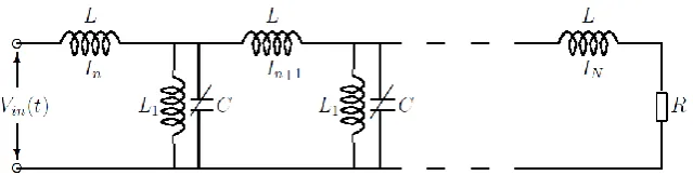
[image:2.595.140.460.486.567.2]Here we describe the electric version of the sine-Gordon–Toda chain. A similar model leading to the discrete and continuous versions of the sine-Gordon model has been studied in (Parmentier, 1978). Consider the transmission line shown in Fig. 1 containing the nonlinear elements, the capacitor whose charge nonlinearly depends on the voltage Q() and inductance L1 with a nonlinear dependence between the current Jn and electric flux n(Jn).
Figure. 1. The ladder-type transmission line with the nonlinear capacitor and inductance L1.
Applying the Kirchhoff’s laws to two neighbor cells with the indices n and n + 1, we obtain:
1
1 ; 1 ;
n n n n n
n n n n n n
n
dQ dI d d dJ
I I J L
dt dt dt dJ dt
, (1)
After simple manipulations this set of equations can be reduced to the set of second-order ODEs:
2
1 1
2 1
2
n n
n n n n
n
d Q dJ
dt L d , (2)
Equations (2) are rather general; making different assumptions regarding Qn(n) and Jn(n), one may obtain various useful and interesting models which are reducible in the long wave approximation to different PDEs.
Consider, for example, the case when
Qn
n Q0ln 1
n a
and dJn d n
r n
sin n b
. (3) Note that in the case of the conventional linear inductive element, the flux n is simply proportional to the current Jn; this case follows from Eq. (3) when n /b << 1, and sin (n /b) n /b.With such choice of the functions Qn(n) and Jn(n) as in Eq. (3) we obtain from Eq. (2):
2
0 2 1 1
ln 1 1
2 sin
n n
n n n
d a
Q r
dt L b
. (4) In the normalized variables, un = n /rL and = t (r /Q0)1/2 Eq. (3) reads
2
1 1
2 ln 1
2 sin
n
n n n n
d u
u u u u
d
, (5) where = rL/a and = rL/b. Equation (5) readily reduces to the classical Toda chain (Toda, 1989) when = 0. In another limiting case when 0 and << 1, one can replace ln (1 + un) un, then Eq. (5) reduces to the discrete sin-Gordon equation (Han, et al., 2008). For the perturbations of infinitely small amplitudes, un 0, Eq. (5) can be linearized:
2
1 1
2 2
n
n n n n
d u
u u u u
d
, (6)
then the dispersion relation can be derived for the sinusoidal perturbations un ~ exp[i( – kn)]: 2 4 2
sin 2
k
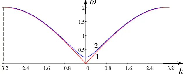
. (7) This dispersion relation is shown in Fig. 2 for = 1 and two values of : = 0 and = 0.05.
3.2
2.4 1.6 0.8 0 0.8 1.6 2.4 3.2 0.5
[image:3.595.156.474.496.623.2]1 1.5 2
Figure. 2. Dispersion relation (7) for = 0 (line 1) and = 0.05 (line 2); = 1 in both cases.
In the long-wave approximation when k << 1 and << k 2 the dispersion relation (7) can be approximated as:
2
2 1
24 2
k k
k
. (8)
This dispersion relation is similar to the dispersion relation describing water waves in rotating fluids (Grimshaw et al., 1998b), and the corresponding nonlinear evolution equation, the Ostrovsky equation, can be derived from the discrete generalized Toda-chain model (5). To demonstrate that, let us assume that the parameter in Eq. (5) is so small that even for the largest possible value of un
k
function sin (un) can be replaced by un with the appropriate accuracy. Assume further that ~ 1 and consider small-amplitude perturbation such that un << 1 for any n. Then Eq. (5) reduces to the following one: 2 2 2 1 1 2 2 2 n
n n n n n
u d
u u u u u
d
. (9)
Consider now a wave with the characteristic wavelength much greater than the spatial size of one cell of the chain (we assume that it is 1), >> 1. Then we can present un 1 through the Taylor series around the node n. Keeping only two non-vanishing leading terms of the Taylor series in the combination un – 1 – 2un + un + 1, we obtain after simple manipulations:
2 2 2 2 4
2 2 2 4
1 1
2 12
u u u u
u
x x
(10)
(index n of the function un(t) has been omitted). In accordance with our assumptions, all terms in the right-hand side of Eq. (10) are small in comparison with the terms in the left-hand side. Therefore, in the zero approximation on small parameters, one can simply neglect the terms in the right-hand side and present the remaining wave equation in the factorized form:
2 2
2 2
1 1 1
0
u u
u
x x x
. (11)
Each bracket in this equation describes independent wave propagating either to the left or to the right. Considering further only a wave propagating to the right, we obtain that in the zero-order approximation the temporal and spatial derivatives are linked by the formula: x , where c0 = 1/√ is the phase velocity of long linear waves. This relationship between the derivatives can be used in the next approximation yielding after substitution into Eq. (10) and simple manipulations the following equation:
3 3
2 24 2
u u u u
u u x
. (12)
This is the well-know Ostrovsky equation which is very popular nowadays in the context of physical oceanography [see for details (Grimshaw et al., 1998b; Stepanyants, 2006)]. When = 0, Eq. (12) reduces to the classical KdV equation which is completely integrable and has a particular solution in the form of stationary solitary wave, alias soliton (Ablowitz & Segur, 1981):
2 1 1
sech , where , .
1 6
x V
u A T V
T A A
(13)
In the next section we consider adiabatic evolution of the KdV soliton under the influence of small perturbation in the right-hand side of Eq. (12) which models influence of Earth’ rotation in the oceanographic context.
Adiabatic evolution of KdV soliton within Ostrovsky Eq. (12)
Assuming that the term in the right-hand side of Eq. (12) is small enough, we can seek for the approximate solution to that equation in the form of KdV soliton with gradually varying parameters in space (amplitude A, velocity V, and duration T). Applying the perturbation method described in (Grimshaw et al., 1998a), one can derive the energy balance equation:
2
, ,
u d u x u x d d
x
. (14)dA A
dx . (15)
This equation can be readily integrated yielding [cf. (Grimshaw et al., 1998a, 1998b]
20 1 t
A x A x X . (16) where A0 is the amplitude of an input soliton entering into the chain at x = 0 and Xt = 2(A0)1/2 / is the terminal length – the length at which the soliton vanishes as its amplitude formally turns to zero. However, in reality the soliton dynamics is more complicated. Numerical calculations show that when the leading soliton decays, it produces an intense trailing perturbation which in turn evolves into another solitary wave of almost the same amplitude as the original soliton was. This secondary soliton is accompanied by trailing wave train too. Then the process of secondary soliton decay repeats with a resurrection of a new soliton and more intense trailing perturbation (Grimshaw et al., 1998b). Such quasi-recurrence phenomenon may occur many times. Eventually, the soliton transfers into the stationary envelope soliton (which can be described by the generalized nonlinear Schrödinger equation) and dispersive wave train. This process has been investigated in details for the KdV soliton within the framework of Ostrovsky equation (Grimshaw & Helfrich, 2008; 2012). Soliton amplitude decay (16) derived within the framework of the adiabatic approximation was compared against numerical solution of the primitive set of Kirchhoff’s Eqs. (1) with the Toda nonlinearity for the charge on the capacitor Qn (n) = Q0 ln(1 + n /a) and linear dependence of the flux n(Jn). Then in the normalized variables the generalized Toda chain model reduces to Eq. (5) with the linear perturbative term un rather than the sinusoidal one. Without loss of generality, one can put in this case = 1, then Eq. (5) with = 0 has the soliton solution (Toda soliton):
2
2
1 1
sech , where , .
ln 1 1 ln
T
n T T T
T T T T T
t n V
u t A T V
T A T T T
(17)
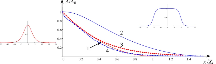
The Toda soliton rapidly reduces to the KdV soliton when its amplitude becomes small AT 0. The primitive set of Kirchhoff’s Eqs. (1) with the functions Qn (n) and n (Jn) indicated above were solved numerically for different values of the parameter . The standard Fortran code was elaborated on the basis of the fourth-order Runge–Kutta solver RKGS with the modification due to Gill. Results obtained are shown in Fig. 3 in normalized variables A(X)/A0 versus X = x /Xt .
0 0.2 0.4 0.6 0.8 1 1.2
[image:5.595.129.507.544.706.2]0.2 0.4 0.6 0.8 1 1.2
Figure. 3. Terminal decay of Toda soliton (17) in the electric chain (5).
Red line 1 shows the theoretical dependence (16) derived in the adiabatic approximation. Dots on that line show the numerical data obtained with A0 = 0.25 and characteristic time duration of the input Toda soliton TT0 = 2. Blue line 2 with small diamonds pertains to the numerical data with A0 =
x/Xt
A/A0
1
0.1 (TT0 = √10), and black line 3 with triangles pertains to numerical data with A0 = 0.5 (TT0 = √2). The parameter = 10–4 in all these cases. As one can see, the numerical data in lines 2 and 3 deviate from the theoretical dependence for the KdV soliton (line 1), although their behavior is qualitatively similar to what is shown by line 1. The data deviation can be explained by inconsistency of the adiabatic theory in application to the numerical data on line 2. Indeed, according to the main assumption of the adiabatic theory, the term in the right-hand side of Eq. (12) should be small in comparison to any term in the left-hand side of that equation. If we roughly estimate the magnitudes of the first term in the left-hand side of Eq. (12) and the right-hand side term we obtain:
2
0 0 0
0 2
0 0 0 0 0
~ ~ ~ ; ~ ,
2 2
T T T T
A A A
u
LHS RHS u A
x T T T T
(18)
where 0 = TT0∙c0 = TT0 / √ is the half-width of the input Toda soliton. Thus, the ratio of the terms in the right-hand side and left-hand side is: RHS/LHS = TT02 /2. As we have put = 1, then for line 1 we have RHS/LHS = 2∙10–4 << 1, whereas for lines 2 and 3 we have correspondingly
RHS/LHS2 = 5∙10–4 and RHS/LHS3 = 10–4. The former of these two values is, apparently, not small enough, whereas the latter one is quite small, but soliton amplitude (A0 = 0.5) is too large which makes difference between the KdV and Toda solitons (the adiabatic theory is developed for the KdV solitons only).
Modeling the Gardner–Ostrovsky equation by means of the modified transmission line
Another choice for the nonlinear dependence between the charge on the capacitor (see Fig. 1) and a voltage Q() = Q0 [/a – (/2)∙(/a)2 – (1/3)∙(/a)3] leads to the chain model similar to that studied in the Fermi–Pasta–Ulam experiments (see, e.g., Ablowitz & Segur, 1981; Toda, 1989). Inclusion of the additional inductance L1 with the nonlinear dependence between the current Jn and electric flux n(Jn) as in Eq. (3) results in the following set of second order ODEs. In the normalised variables, un = n /rL, = t (r /Q0)1/2 the set reads
2
2 1 3
1 1
2 2 sin
2 2
n n n n n n n
d
u u u u u u u
d
, (19)
where and 1 are some coefficients. Assuming un << 1 (so that sin(un) ≈ un) and repeating the manipulations undertaken above in the derivation of the Ostrovsky equation, one can reduce the set of ODEs (19) to the well-known Gardner–Ostrovsky equation (Holloway et al., 1999; Grimshaw et al, 2006; Obregon, Stepanyants, 2012):
2 3
2
1 3
2 2 24 2
u u u u u
u u u
x
. (20)
When = 0 this equation reduces to the Gardner (or extended KdV) equation which is completely integrable and also has soliton solutions (see, e.g., Apel et al., 2007). However, the structure of Gardner solitons is different from the structure of KdV solitons and essentially depends on the sign of the parameter 1, whereas the parameter controls only the polarity of the Gardner soliton. In particular, the Gardner soliton with 1 < 0 and > 0 has a positive polarity:
1
tanh tanh
2 G G
x V x V
u
T T
where soliton amplitude A = – /1, velocity V = (1 + 2 2/121)–1/, characteristic duration TG = (–21)1/2/||, as well as 0.25ln 1
/ 1
are determined by the parameter (0, 1).Under small perturbation in the right-hand side of Eq. (20) when ≠ 0 the Gardner soliton gradually decays. From the energy balance equation (14) it follows the equation for the parameter v:
2 2
1 1
ln
4 1
d d
. (22)
Unfortunately, this equation is not solvable analytically in general, however it can be readily solved numerically or asymptotically for 0 (KdV limit) and 1 (table-top limit). The results obtained are shown in Fig. 4. Line 1 in that figure pertains to the KDV limit which corresponds to Eq. (16), whereas line 2 pertains to the table-top limit (obtained numerically by solving Eq. (22)).
[image:7.595.70.525.300.436.2]
Figure. 4. Terminal decay of the Gardner soliton (21) in the electric chain (19). Bell-shaped pulse in the left insertion corresponds to KdV soliton of a unit amplitude, and wide pulse in
the right insertion illustrates table-top soliton of a unit amplitude.
The theoretical results derived within the adiabatic approximation were compared against numerical data obtained from the direct solution of Eq. (19) with the Gardner soliton as the input signal. The following parameters of Eq. (19) were chosen: = – 1 = 0.1, = 1, and = 10
–4
. It was confirmed that for small and moderate soliton amplitudes, the decay law caused by small perturbative factor in the right-hand side of Eq. (19) agrees well with the theoretical prediction (see, e.g., line 3 in Fig. 4 which is obtained for 0 = 0.5). However, numerical data for large-amplitude table-top solitons are far from the theoretical prediction (see line 4 which pertain to the case of 0 = 1 – 10–7). The detailed inspection of soliton evolution shows that contrary to theoretical assumption, the table-top soliton decays not preserving its shape even at very early stage of the evolution (see Fig. 5).
Conclusions
As has been shown in this paper, chain models can be used for the effective modeling partial differential equations describing nonlinear wave processes in continuous dispersive media. Dissipative terms can be also taken into account; this does not make any additional difficulty, whereas the numerical solution of PDEs containing both dispersive and dissipative terms is not so simple problem. We obtained the results on KdV soliton decay within the framework of Ostrovsky equation (12) and demonstrated that within the range of applicability of the adiabatic theory, our numerical results agree fairly well with the theoretical predictions. In the meantime, it was revealed that the table-top Gardner soliton does not obey the adiabatic theory. It decays much faster at the earlier stage due to transformation into bell-shaped pulse rather than preserving its own shape. This
x /Xt
A/A0
1
2 3 4
20
15 10 5 0 5 10 15 20 0.5
1
40
30 20 10 0 10 20 30 40 0.5
1
0 0.2 0.4 0.6 0.8 1 1.2 1.4 1.6
is in contrast to what was discovered for the adiabatic decay of Gardner soliton due to different dissipative perturbations (Grimshaw et al., 2003). Evidently, the non-dissipative perturbation considered in this paper and modeling the effect of Earth’ rotation in physical oceanography affects differently on such solitons than the dissipative perturbations. This issue will be studied in details subsequently.
0 200 400 600
0.5
0.5 1
Fig. 5. Time dependence of the signal generated by the table-top Gardner soliton (21) with 0 = 1 – 10–7 in different cells of the electric lattice (19). Line 1 shows the input pulse, line 2
pertains to n = 100, line 3 – to n = 200, line 4 – to n = 300, line 5 – to n = 400.
References
Ablowitz, M. J. and Segur, H. (1981), Solitons and the Inverse Scattering Transform, SIAM, Philadelphia.
Apel, J., Ostrovsky, L.A., Stepanyants, Y.A., and Lynch, J.F. (2007), Internal solitons in the ocean and their effect on underwater sound. J. Acoust. Soc. Am., 121, n. 2, pp. 695–722.
Dodd, R. K., Eilbeck, J. C., Gibbon, J. D., and Morris, H. C. (1982), Solitons and Nonlinear Wave Equations. Academic Press, London.
Grimshaw, R. H. J., He, J.-M., and Ostrovsky, L. A. (1998a), Terminal damping of a solitary wave due to radiation in rotational systems. Stud. Appl. Math., 101, pp. 197–210.
Grimshaw, R., Ostrovsky, L. A., Shrira, V.I., and Stepanyants, Yu. A. (1998b), Long nonlinear surface and internal gravity waves in a rotating ocean. Surveys in Geophys., 19, pp. 289–338.
Grimshaw, R., Pelinovsky, E. N., and Talipova, T. G. (2003), Damping of large-amplitude solitary waves. Wave Motion, 37, pp. 351–364.
Grimshaw, R., Pelinovsky, E., Stepanyants, Y., and Talipova, T. (2006) Modeling internal solitary waves on the Australian North West Shelf. Marine and Freshwater Research, 57, pp. 265–272.
Grimshaw, R. and Helfrich, K. (2008), Long-time solutions of the Ostrovsky equation. Stud. Appl. Math., 121, pp. 71– 88; (2012), The effect of rotation on internal solitary waves. IMA J. Appl. Math. 77 (to be published).
Han, H, Zhang, J., and Brunner, H. (2008), Numerical soliton solutions for a discrete sin-Gordon system. ICM Research Report 08–16, Institute for Computational Mathematics, Hong Kong Baptist University, 16 pp.
Holloway, P., Pelinovsky, E., and Talipova, T. (1999), A generalised Korteweg–de Vries model of internal tide transformation in the coastal zone. Geophys Research, 104, n. 18, pp. 333–350.
Lonngren, K. E. (1978), Observation of solitons on a nonlinear transmission lines. In:K. Lonngren and A. C. Scott (eds.), Solitons in Action. Academic Press, New York.
Obregon, M. and Stepanyants, Y. (2012), On numerical solution of the Gardner–Ostrovsky equation. Mathematical Modelling of Natural Phenomena, 7, n. 2, pp. 113–130.
Parmentier, R. D. (1978), Fluxons in long Josephson junctions. In: K. Lonngren and A.C. Scott (eds.), Solitons in Action. Academic Press, New York, pp. 173–199.
Rabinovich, M. I. and Trubetskov, D. I. (1989), Oscillations and Waves in Linear and Nonlinear Systems. Kluwer Academic, Dordrecht.
Stepanyants, Yu. A. (1981), Experimental investigation of cylindrically diverging solitons in an electric lattice. Wave Motion, 3, n. 4, pp. 335–341.
Toda, M. (1989), Theory of Nonlinear Lattices (2-nd ed.), Springer, Berlin.
Zolotaryuk, Y., Savin, A.V., and Christiansen, P. L. (1988), Solitary plane waves in an isotropic hexagonal lattice.
Phys. Rev. B, 57, n. 22, pp. 14213–14227.
un ()