A novel multiobjective evolutionary algorithm based on regression analysis

(1)

Research Article

A Novel Multiobjective Evolutionary Algorithm

Based on Regression Analysis

Zhiming Song,

1

Maocai Wang,

1,2

Guangming Dai,

1

and Massimiliano Vasile

2 1_{School of Computer, China University of Geosciences, Wuhan 430074, China}

2_{Department of Mechanical & Aerospace Engineering, University of Strathclyde, Glasgow G1 1XJ, UK}

Correspondence should be addressed to Maocai Wang; [email protected]

Received 23 June 2014; Revised 15 September 2014; Accepted 30 December 2014

Academic Editor: Shifei Ding

Copyright © 2015 Zhiming Song et al. This is an open access article distributed under the Creative Commons Attribution License, which permits unrestricted use, distribution, and reproduction in any medium, provided the original work is properly cited.

As is known, the Pareto set of a continuous multiobjective optimization problem with𝑚objective functions is a piecewise continuous (𝑚 − 1)-dimensional manifold in the decision space under some mild conditions. However, how to utilize the regularity to design multiobjective optimization algorithms has become the research focus. In this paper, based on this regularity, a model-based multiobjective evolutionary algorithm with regression analysis (MMEA-RA) is put forward to solve continuous multiobjective optimization problems with variable linkages. In the algorithm, the optimization problem is modelled as a promising area in the decision space by a probability distribution, and the centroid of the probability distribution is (𝑚 − 1)-dimensional piecewise continuous manifold. The least squares method is used to construct such a model. A selection strategy based on the nondominated sorting is used to choose the individuals to the next generation. The new algorithm is tested and compared with NSGA-II and RM-MEDA. The result shows that MMEA-RA outperforms RM-MEDA and NSGA-II on the test instances with variable linkages. At the same time, RA has higher efficiency than the other two algorithms. A few shortcomings of MMEA-RA have also been identified and discussed in this paper.

1. Introduction

Evolutionary algorithm has become an increasingly popular

design and optimization tool in the last few years [1].

Although there have been a lot of researches about evolution-ary algorithm, there are still many new areas that needed to be explored with sufficient depth. One of them is how to use the evolutionary algorithm to solve multiobjective optimization problems. The first implementation of a multiobjective

evolu-tionary algorithm dates back to the mid-1980s [2]. Since then,

many researchers have done a considerable amount of works in the area, which is known as multiobjective evolutionary algorithm (MOEA).

Because of the ability to deal with a set of possible solu-tions simultaneously, evolutionary algorithm seems particu-larly suitable to solve multiobjective optimization problems. The ability makes it possible to search several members of

the Pareto-optimal set in a single run of the algorithm [3].

Obviously, evolutionary algorithm is more effective than the

traditional mathematical programming methods in solving multiobjective optimization problem because the traditional

methods need to perform a series of separate runs [4].

The current MOEA research mainly focuses on some

highly related issues [5]. The first issue is the fitness

assign-ment and diversity maintenance. Some techniques such as fitness sharing and crowding have been frequently used to maintain the diversity of the search. The second issue is the external population. The external population is used to record nondominated solutions found during the search. There have been some efforts on how to maintain and utilize such an external population. The last issue is the combination of MOEA and local search. Researches have shown that the combination of evolutionary algorithm and local heuristics search outperforms traditional evolutionary algorithms in a

wide variety of scalar objective optimization problems [4,6].

However, there are little researches focusing on the way to generate new solutions in MOEA. Currently, most MOEAs directly adopt traditional genetic operators such as crossover

(2)

and mutation. These methods have not fully utilized the characteristics of MOP when generating new solutions. Some researches show that MOEA fails to solve MOPs with variable linkages, and the recombination operators are crucial to the

performance of MOEA [7]. It has been noted that under mild

smoothness conditions, the Pareto set (PS) of a continuous

MOP is a piecewise continuous (𝑚 − 1)-dimensional

man-ifold, where 𝑚 is the number of the objectives. However,

as analyzed in [8], this regularity has not been exploited

explicitly by most current MOEA.

In 2005, Zhou et al. proposed to extract regularity patterns of the Pareto set by using local principal component

analysis (PCA) [9]. They had also studied two naive hybrid

MOEAs. In the two MOEAs, some trial solutions were gener-ated by traditional genetic operators and others by sampling from probability models based on regularity patterns in 2006

[10].

In 2007, Zhang et al. conducted a further and thorough

investigation along their previous works in [9, 10]. They

proposed a regularity model-based multiobjective estimation

of distribution algorithm and named it as RM-MEDA [5]. At

each generation, the proposed algorithm models a promising area in the decision space by a probability distribution whose

centroid is a (𝑚 − 1)-dimensional piecewise continuous

manifold. The local principal component analysis algorithm is used to build such a model. Systematic experiments have shown that RM-MEDA outperforms some other algorithms on a set of test instances with variable linkages.

In 2008, Zhou et al. proposed a probabilistic model based multiobjective evolutionary algorithm to approximate PS and PF (Pareto front) for a MOP in this class simultaneously

and named the algorithm as MMEA [11]. They proposed two

typical classes of continuous MOPs as follows. One class is that PS and PF are of the same dimensionality while the other

one is that PF is a (𝑚 − 1)-dimensional continuous manifold

and PS is a continuous manifold with a higher dimensionality. There is a class of MOPs, in which the dimensionalities of PS and PF are different so that a good approximation to PF might not approximate PS very well. MMEA could promote the population diversity both in the decision spaces and in the objective spaces.

Modeling method is a crucial part for MOEA because it determines the performance of the algorithms. Zhang et al. built such a model by local principal component analysis

(PCA) algorithm [5]. The test results show that the method

has great performance over some instances with linkage variables. However, there are still some shortcomings about the method. The first shortcoming is that RM-MEDA needs extra CPU time for running local PCA at each generation. The second one is that the model is just linear fitting for all types of PS, including the one with nonlinear linkage variables, which enable that the result may be not accurate.

In the paper, we proposed a model-based multiobjective evolutionary algorithm with regression analysis, which is named as MMEA-RA. In MMEA-RA, a new modeling method based on regression analysis is put forward. In the method, least squares method (LSM) is used to fit a 1-dimensional manifold in high-1-dimensional space. Because least squares can fit any type of curves through its model,

the shortcomings of RM-MEDA can be avoided, especially for the instances with nonlinkage variables.

The rest of this paper is organized as follows. After defin-ing the continuous multiobjective optimization problem in

Section 2, the new model of multiobjective evolutionary algorithm based on regression analysis is put forward in

Section 3. Then, a description of the test cases for

MMEA-RA follows inSection 4. After presenting the results of the

tests, the performance of MMEA-RA is analyzed and some

conclusions are given inSection 5.

2. Problem Definition

In this paper, the continuous multiobjective optimization

problem is defined as follows [5]:

min 𝐹 (𝑥) = (𝑓₁(𝑥) , 𝑓₂(𝑥) , . . . , 𝑓_𝑚(𝑥))𝑇

s.t. 𝑥 = (𝑥₁, . . . , 𝑥_𝑛)𝑇∈ 𝑋,

(1)

where𝑋 ⊂ 𝑅𝑛is the decision space and𝑥 = (𝑥₁, . . . , 𝑥_𝑛)𝑇is

the decision vector.𝐹 : 𝑋 → 𝑅𝑚consists of𝑚real-valued

continuous objective functions𝑓_𝑖(𝑥) (𝑖 = 1, . . . , 𝑚).𝑅𝑚is the

objective space.

Let𝑎 = (𝑎₁, . . . , 𝑎_𝑛)𝑇 ∈ 𝑅𝑛and𝑏 = (𝑏₁, . . . , 𝑏_𝑛)𝑇 ∈ 𝑅𝑛be

two vectors, and𝑎is said to dominate𝑏, denoted by𝑎 ≺ 𝑏,

if𝑎_𝑖 ≤ 𝑏_𝑖for all𝑖 = 1, . . . , 𝑛, and𝑎 ̸= 𝑏. A point𝑥∗ ∈ 𝑋is

called (globally) Pareto optimal if there is no𝑥 ∈ 𝑋such that

𝐹(𝑥) ≺ 𝐹(𝑥∗₎_{. The set of all Pareto-optimal points, denoted}

by PS, is called the Pareto set. The set of all Pareto objective vectors is called the Pareto front, denoted by PF.

3. Algorithm

3.1. Basic Idea. Under certain smoothness assumptions, it can be induced from the Karush-Kuhn-Tucker condition that the PS of a continuous MOP defines a piecewise continuous (𝑚 − 1)-dimensional manifold in the decision space [12]. Therefore, the PS of a continuous biobjective optimization

problem is a piecewise continuous curve in𝑅2.

The population in the decision space in a MOEA for

(1) will hopefully approximate the PS and is uniformly

scattered around the PS as the search goes on. Therefore, we can envisage the points in the population as independent

observations of a random vector𝜉 ∈ 𝑅𝑛 whose centroid is

the PS of(1). Since the PS is a (𝑚 − 1)-dimensional piecewise

continuous manifold,𝜉can be naturally described by

𝜉 = 𝜁 + 𝜀, (2)

where𝜁is uniformly distributed over a piecewise continuous

(𝑚 − 1)-dimensional manifold, and 𝜀 is an𝑛-dimensional

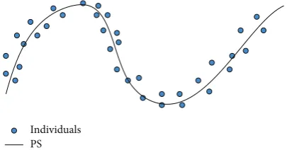
zero-mean noise vector.Figure 1illustrates the basic idea.

(3)

[image:3.600.69.272.73.179.2]

Individuals PS

Figure 1: Individual solutions should be scattered around the PS in the decision space in a successful MOEA.

optimization problems with variable linkages. The algorithm is named as MMEA-RA. The algorithm works as follows.

MMEA-RA

Step 1(initializing). Set𝑡 = 0. Generate an initial population

Pop(0)and compute the value𝐹of each individual solution

in Pop(0).

Step 2(stopping). If stopping condition is met, the algorithm

stops and returns the nondominated solutions in Pop(𝑡), and

their corresponding𝐹vectors constitute an approximation to

the PF.

Step 3(modeling). Build the probability model in Pop(𝑡)to

fit expression(2),

(3.1) to compute the coefficients𝑎_𝑘for 𝑘 = 0, 1, . . . , 𝑗by

solving the matrix in expression(10);

(3.2) to compute the manifold𝜓 = {𝑥 = (𝑥₁, . . . , 𝑥_𝑛) ∈ 𝑅𝑛}

by expression(11);

(3.3) to generate a𝑛-dimensional zero-mean noise vector

between (−noise,noise) randomly based on

expres-sions(13)and(14).

Step 4(reproducing). Generate a new solution set 𝑄from

expression(2). Evaluate the value𝐹of each solution in𝑄.

Step 5(selecting). Select𝑁individuals from𝑄 ∪Pop(𝑡)to

create Pop(𝑡 + 1).

Step 6. Set𝑡 = 𝑡 + 1and go to Step 2.

In the followingSection 3.3, the implementation of

mod-eling, reproducing, and selecting of the above algorithm will be given in detail.

3.3. Modeling. Fitting expression(2)to the points in Pop(𝑡) is highly related to principal curve analysis, which aims at

finding a central curve of a set of points in𝑅𝑛[13]. However,

most current algorithms for principal curve analysis are rather expensive due to the intrinsic complexity of their

models. RM-MEDA uses the (𝑚 − 1)-dimensional local

principal component analysis (PCA) algorithm [14]; it is

less complex compared with most algorithms for principal

y

x z

l

Projection of the line_l

Projection of the linel

O

on planexOz:x = az + c

on planeyOz:y = bz + d

Figure 2: Illustration of the geometric meaning of expression(3).

curve analysis. However, it needs much more CPU time compared with the traditional evolutionary algorithms which adopt genetic recombination operators such as crossover and mutation. Moreover, the PS cannot be exactly described by local PCA because it only uses linear curves to approximate

the model at one cluster of Pop(𝑡).

In this implementation, we do not make use of clustering method in the modeling process. We try to find the principal

curve of the whole points in Pop(𝑡), not just the local part

of them. As is known, least squares approach is a simple and effective method for linear curve fitting and nonlinear curve fitting, such as polynomial or exponential curve fitting. Then we consider whether this technique could be made use of to

describe expression(2).

For the sake of simplicity, it could be assumed that the

centroid of𝜉is a manifold𝜓in formula(2), and𝜁is uniformly

distributed on𝜓.𝜓is a (𝑚 − 1)-dimensional hyperrectangle.

Particularly, in the case of two objectives,𝜓is a curve segment

in𝑅2.

A line in 3-dimensional space can be expressed as

𝑥 = 𝑎𝑧 + 𝑐, 𝑦 = 𝑏𝑧 + 𝑑, (3)

where𝑎, 𝑏, 𝑐, and𝑑are the coefficients of the expression.

The geometric meaning of expression (3) is that a

3-dimensional line𝑙can be seen as the intersecting line of two

planes𝑚₁:𝑥 = 𝑎𝑧 + 𝑐and𝑚₂:𝑦 = 𝑏𝑧 + 𝑑.Figure 2illustrates

this meaning.

The expression𝑥 = 𝑎𝑧 + 𝑐can be seen as the projection of

the line𝑙in𝑥𝑂𝑧plane, and𝑦 = 𝑏𝑧 + 𝑑is the one in the𝑦𝑂𝑧

plane.

As a 3-dimensional line can be expressed by the

intersect-ing of 2 planes, then a𝑛-dimensional line can be expressed as

the intersecting of (𝑛 − 1) planes as

𝑥₂= 𝑎₁+ 𝑏₁𝑥₁, 𝑥₃= 𝑎₂+ 𝑏₂𝑥₁,

...

𝑥_𝑛= 𝑎_𝑛−1+ 𝑏_𝑛−1𝑥₁.

(4)

Expression 𝑥_𝑖 = 𝑎_𝑖−1 + 𝑏_𝑖−1𝑥₁ can be regarded as the

[image:3.600.311.546.73.154.2]

(4)

x y

for entire range

f(x) = ax + b

(a)

x y

for entire range

f(x) = ax2+ bx + c

[image:4.600.100.504.69.244.2]

(b)

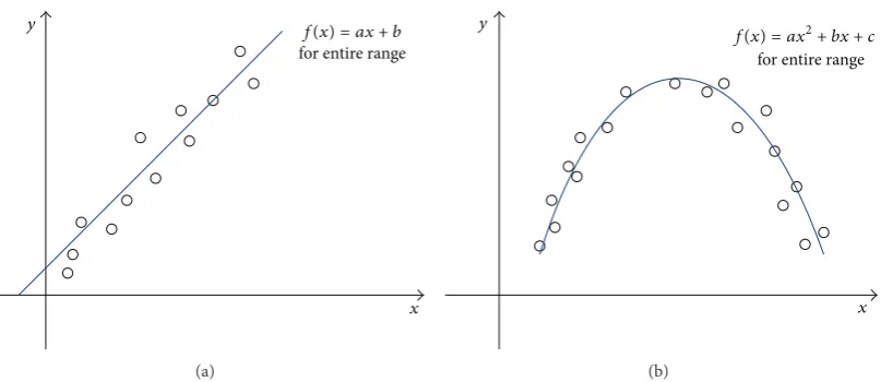
Figure 3: Illustration of the least squares approach (a) linear (b) nonlinear.

By expression(4), we further conclude that a𝑛

-dimen-sional curve can be regarded as the intersecting of (𝑛 − 1)

surface, and expression(5)shows this idea:

𝑥2= 𝑎1,0+ 𝑎1,1𝑥1+ 𝑎1,2𝑥21+ ⋅ ⋅ ⋅ + 𝑎1,𝑝𝑥𝑝1,

𝑥₃= 𝑎_2,0+ 𝑎_2,1𝑥₁+ 𝑎_2,2𝑥2₁+ ⋅ ⋅ ⋅ + 𝑎_2,𝑝𝑥𝑝₁, ...

𝑥𝑛= 𝑎𝑛−1,0+ 𝑎𝑛−1,1𝑥1+ 𝑎𝑛−1,2𝑥21+ ⋅ ⋅ ⋅ + 𝑎𝑛−1,𝑝𝑥𝑝1.

(5)

Expression𝑥_𝑗 = 𝑎_𝑗−1,0+ 𝑎_𝑗−1,1𝑥₁+ 𝑎_𝑗−1,2𝑥2₁+ ⋅ ⋅ ⋅ + 𝑎_{𝑗−1,𝑝}𝑥𝑝₁

can be regarded as the approximate projection of the 𝑛

-dimensional curve in𝑥_𝑗𝑂𝑥₁surface. Each expression is a𝑝

-order polynomial.(𝑥₁, . . . , 𝑥_𝑛)is a point on the𝑛-dimensional

curve. Then the thing that we need to do is to find out all the

coefficients𝑎_𝑖,𝑗, which could make the curve fit the population

in the decision space well, and here we used least squares approach method to help us find out the best coefficients.

Least squares approach is mainly used to fit the curve, that is to say, to capture the trend of the data by assigning a single

function across the entire range.Figure 3shows the idea.

InFigure 3,Figure 3(a)looks linear in trend, so we can fit the curve by choosing a general form of the straight line

𝑓(𝑥) = 𝑎𝑥 + 𝑏, and then the goal is to identify the coefficients

𝑎and𝑏such that𝑓(𝑥)fits the date well, the method to identify

the two coefficients is called as linear regression.Figure 3(b)

looks nonlinear, we use higher polynomial 𝑓(𝑥) = 𝑎𝑥2 +

𝑏𝑥 + 𝑐, and the goal is to find out the coefficients𝑎, 𝑏, and

𝑐such that𝑓(𝑥) fits the date well. It is called as nonlinear

regression compared with linear regression. In fact, there are a lot of functions with different shapes that depend on the coefficients. The methods to find out the best coefficients are just called as regression analysis (RA).

Consider the general form for a polynomial with order𝑗:

𝑓 (𝑥) = 𝑎0+ 𝑎1𝑥 + 𝑎2𝑥2+ ⋅ ⋅ ⋅ + 𝑎𝑗𝑥𝑗 = 𝑗 ∑ 𝑘=0

𝑎𝑘𝑥𝑘. (6)

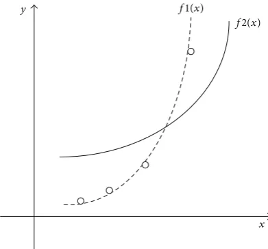
How can we choose the coefficients that best fit the curve to the data? The idea of least squares approach is to find

a curve that gives minimum error between data𝑦and the

fitting curve𝑓(𝑥). As is shown inFigure 4, we can firstly add

up the length of all the solid and dashed vertical lines and then pick curve with minimum total error. The general expression for any error using the least squares approach is

err=

𝑛 ∑ 𝑖=1

(𝑑_𝑖)2= (𝑦₁− 𝑓 (𝑥₁))2+ (𝑦₂− 𝑓 (𝑥₂))2

+ ⋅ ⋅ ⋅ + (𝑦_𝑛− 𝑓 (𝑥_𝑛))2.

(7)

For expression(7), we want to minimize the error err. Replace

𝑓(𝑥)in expression(7)with the expression(6), and then we

have

err=

𝑛 ∑ 𝑖=1

(𝑦_𝑖−∑𝑗 𝑘=0

𝑎_𝑘𝑥𝑘_𝑖) 2

, (8)

where𝑛is the number of data points given,𝑖is the current

data points being summed, and𝑗is the polynomial order. To

find the best line means to minimize the square of the distance error between line and data points. Find the set of coefficients

𝑎₀, 𝑎₁, . . . , 𝑎_𝑗, that is to say, to minimize expression(8). In Figure 4, there are four data points and two fitting

curves 𝑓1(𝑥) and 𝑓2(𝑥). Obviously, 𝑓1(𝑥) is better than

𝑓2(𝑥)because there is smaller error between the four points

and the fitting curve𝑓1(𝑥).

To minimize expression (8), take the derivative with

respect to each coefficient𝑎_𝑘for𝑘 = 0, 1, . . . , 𝑗, and set each

to zero:

𝜕err

𝜕𝑎₀ = − 2 𝑛 ∑ 𝑖=1

(𝑦_𝑖−∑𝑖 𝑘=0

𝑎_𝑘𝑥𝑘) = 0,

𝜕err

𝜕𝑎₁ = − 2 𝑛 ∑ 𝑖=1(𝑦𝑖−

𝑖 ∑ 𝑘=0

(5)

x

y f1(x)

[image:5.600.71.267.72.254.2]

f2(x)

Figure 4: Four data points and two different curves.

... 𝜕err

𝜕𝑎_𝑗 = − 2 𝑛 ∑ 𝑖=1

(𝑦_𝑖−∑𝑖 𝑘=0

𝑎_𝑘𝑥𝑘) 𝑥𝑗= 0.

(9)

Rewrite these𝑗 + 1equations, and put into matrix form:

( ( (

(

𝑛 ∑ 𝑥_𝑖 ∑ 𝑥2

𝑖 ⋅ ⋅ ⋅ ∑ 𝑥𝑗𝑖 ∑ 𝑥_𝑖 ∑ 𝑥2_𝑖 ∑ 𝑥_𝑖3 ⋅ ⋅ ⋅ ∑ 𝑥𝑗+1_𝑖

...

∑ 𝑥𝑗_𝑖 ∑ 𝑥𝑗+1_𝑖 ∑ 𝑥𝑗+2_𝑖 ⋅ ⋅ ⋅ ∑ 𝑥𝑗+𝑗_𝑖 ) ) )

) (

( 𝑎₀ 𝑎1 ... 𝑎_𝑗

)

= ( ∑ 𝑦_𝑖 ∑ 𝑥_𝑖𝑦_𝑖

... ∑ 𝑥𝑗_𝑖𝑦𝑖

) .

(10)

The coefficients 𝑎_𝑘 for 𝑘 = 0, 1, . . . , 𝑗can be solved by

matrix computation.

With the above work, we can describe the 1-dimensional

manifold𝜓as

𝜓 ={_{ {

𝑥 = (𝑥₁, . . . , 𝑥_𝑛) ∈ 𝑅𝑛 _|

𝑥_𝑖=∑𝑝 𝑗=0

𝑎_{𝑖−1,𝑗}𝑥𝑗₁, 𝑎₁− 0.25 (𝑏₁− 𝑎₁)

≤ 𝑥₁≤ 𝑏₁+ 0.25 (𝑏₁− 𝑎₁) , 𝑖 = 2, . . . , 𝑛}_} } ,

(11)

Pareto set

𝜓

𝜓󳰀

Figure 5: Illustration of extension.

where𝑝is the polynomial order and𝑎₁and𝑏₁are the

mini-mum and maximini-mum values on𝑥₁:

𝑎₁= min

1≤𝑗≤𝑁𝑥 𝑗

1, 𝑏1=_{1≤𝑗≤𝑁}max𝑥𝑗1. (12)

In order to approximate the PS better,𝜓is extended by

50% along𝑥₁.Figure 5shows this idea. InFigure 5,𝜓󸀠could

not approximate the PS very well, but its extension 𝜓can

provide a better approximation.

When we find out the coefficients𝑎_𝑖,𝑗 (𝑖 = 1, . . . , 𝑛−1, 𝑗 =

0, . . . , 𝑝) based on least square approach above, we could

get𝜁in expression(2).𝜁is generated over𝜓uniformly and

randomly.

In expression(2),𝜀is a𝑛-dimensional zero-mean noise

vector, and it is designed as the following description:

𝜀 = (𝜀₁, 𝜀₂, . . . , 𝜀_𝑛) , (13)

where𝜀_𝑖 is a random number between (−noise,noise). The

noise is changed from big to small as the generation goes on because big noise can accelerate the convergence of the pop-ulation in the early generation and small noise can maintain

the accuracy of the population in the end. Expression(14)

shows the implementation:

noise= 𝐹₀∗ 10𝑒(1−maxGen/(maxGen+1−curGen)), (14)

where maxGen is the max generation of the algorithm and

is set to be 200 and curGen is the current generation.𝐹₀ is

set to be 0.2 when the algorithm begins. Then the noise is changed from 0.2 to 0.02. The trends of the noise can be seen inFigure 6. As is shown inFigure 6, the noise decreases as the generation increases, and it will be stable after the 160th generation.

3.4. Reproducing. It is desirable that final solutions are uni-formly distributed on the PS. Therefore, in order to maintain the diversity of the solution, in this paper, the new solution is generated uniformly and randomly as follows.

[image:5.600.63.294.401.556.2]

(6)

Table 1: Test instance.

Test case Variables Objectives

𝑇1 [0, 1]𝑛× [0, 10]𝑛−1

𝑓1(𝑥) = 𝑥1

𝑓₂(𝑥) = 𝑔 (𝑥) [1 − √𝑓1(𝑥)

𝑔 (𝑥)] 𝑔 (𝑥) = ₄₀₀₀1 ∑𝑛

𝑖=2

(𝑥2

𝑖− 𝑥1)2−

𝑛

∏

𝑖=2

cos(𝑥

2

𝑖− 𝑥1

√𝑖 − 1) + 2

The trends of the noise

N

o

is

e val

u

e

Current generation

0.2

0.18

0.16

0.14

0.12

0.1

0.08

0.06

0.04 0.02

[image:6.600.50.289.125.373.2]

0 20 40 60 80 100 120 140 160 180 200

Figure 6: The trends of the noise.

Step 2. Generate a noise vector𝜀󸀠in expression(13).

Step 3. Return𝑥 = 𝑥󸀠+ 𝜀󸀠.

In Step 3 of the algorithm framework of MMEA-RA,𝑁

new solutions can be produced by repeating above all steps

𝑁times.

3.5. Selecting. The selection procedure used in this paper is

the same in the procedure used in [5], which is based on

the nondominated sorting of NSGA-II [15]. The selection

procedure is called as NDS-selection.

The main idea of NDS-selection is to divide𝑄 ∪Pop(𝑡)

into different fronts𝐹₁, 𝐹₂, . . . , 𝐹_𝑙 such that the𝑗th front𝐹_𝑗

contains all the nondominated solutions in{𝑄 ∪Pop(𝑡)} \

(⋃𝑗−1_𝑖=1𝐹_𝑖). Therefore, there is no solution in{𝑄 ∪Pop(𝑡)} \

(⋃𝑗−1_𝑖=1𝐹𝑖) that could dominate a solution in 𝐹𝑗. Roughly

speaking,𝐹₁is the best nondominated front in𝑄 ∪Pop(𝑡),

and𝐹₂is the second best nondominated front, and so on. The

detailed procedure of NDS-selection can be found in [5].

4. Test Case

4.1. Performance Metric. In this paper, the performance metric used to evaluate the solutions is the convergence

metric𝛾, which is also the common performance metric in

multiobjective optimization algorithm [16].

The metric𝛾measures that the solutions will be

conver-gent to a known set of Pareto-optimal solutions. We find a set of 500 uniformly solutions from the true Pareto-optimal front in the objective space. And then to compute the minimum Euclidean distance of each solution from chosen solutions on the Pareto-optimal front. The average of theses distances is

used as the metric𝛾.

4.2. General Experimental Setting. There are three algorithms employed to solve the test instance for a comparison. These three algorithms are RM-MEDA, NSGA-II, and MMEA-RA, while MMEA-RA is the new algorithm proposed in this paper.

The three algorithms are implemented by C++. The ma-chine used in the test is Core 2 Duo (2.4 GHz, 2.00 GB RAM). The experiment setting is as follows.

The number of new trial solutions generated at each generation is set to be 100 for all tests.

The number of decision variables is set to be 30 for all tests.

Parameter setting in RM-MEDA: the number of

cluster𝐾is set to be 5 in local PCA algorithm.

Parameter setting in MMEA-RA: the order is set to be 2.

We run each algorithm independently 10 times for the test instance. The algorithms stop after a given number of generations. The maximal number of generations in three algorithm is 1000.

Table 1 gives the test instance [5]. In the test instance, the feasible decision space is a hyperrectangle. There are nonlinear variable linkages in the test case. Furthermore, the test instance has many local Pareto fronts since its

𝑔(𝑥) has many locally minimal points. It also has some

characteristics such as concave PF, nonlinear variable linkage, and multimodal with Griewank function.

If an element of solution𝑥, sampled from MMEA-RA or

RM-MEDA, is out of the boundary, we simply reset its value to a randomly selected value inside the boundary.

4.3. Performance Analysis. The evolution of the average𝛾 -metric of the nondominated solutions for the test case is

shown inFigure 7. It should be noted that the solutions of

(7)

0 100 200 300 400 500 600 700 800 900 Number of generations

C

o

n

ver

ge

nce val

u

e

MMEA-RA RM-MEDA NSGA-II

102

101

100

10−1

10−2

10−3

T1

Figure 7: The evolution of the average𝛾-metric of the nondomi-nated solutions in three algorithms for𝑇1.

solution from chosen solutions as the metric𝛾, the smaller the

convergence values, the better the convergence metric𝛾. As

is shown byFigure 7, among the three algorithms,

MEMA-RA has best convergence performance and NSGA-II and RM-MEDA follow.

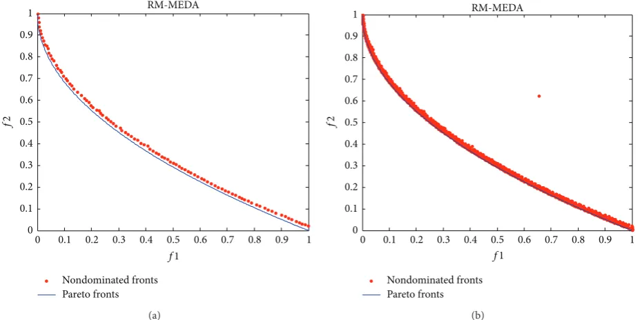
Figure 8 shows the final nondominated solutions and

fronts obtained by MMEA-RA on the test case.Figure 8(a)is

the result with the lowest𝛾-metric obtained in 10 runs while

Figure 8(b)is all the 10 fronts in 10 runs. It can be seen that

the nondominated fronts with the lowest𝛾-metric are very

close to the Pareto front, especially when𝑓1tends to 0 and

𝑓2tends to 1. It can also be noted that the nondominated

solutions in every run have some small fluctuations around the Pareto front.

The final nondominated solutions and fronts obtained by

RM-MEDA on the test case are shown inFigure 9. Similarly,

Figure 9(a)is the result with the lowest𝛾-metric obtained in

10 runs whileFigure 9(b)gives all the 10 fronts in 10 runs.

Similar toFigure 8, the nondominated solution(s) in Figures

9(a) and 9(b) are marked with red. The Pareto fronts are

marked with blue. The Pareto fronts are given in Figures9(a)

and9(b)only for comparing the quality of the nondominated

solutions. It can be seen that the nondominated front with

the lowest𝛾-metric is very consistent with the Pareto front

although there are some differences between them. In partic-ular, it should be noted that all results in 10 runs from RM-MEDA match the Pareto front better than MMEA-RA. But it also should be noted that there is an isolated point in the

nondominated solutions for all 10 runs inFigure 9(b), maybe

because RM-MEDA falls into a local minimum and could not jump out.

The final nondominated solutions and fronts obtained

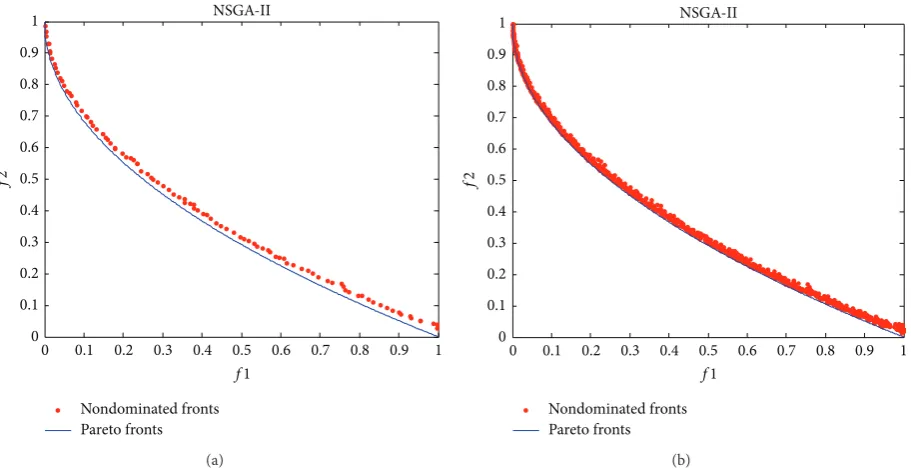
by NSGA-II on the test case are shown inFigure 10. Again,

[image:7.600.56.288.70.301.2]

Figure 10(a) means the result with the lowest 𝛾-metric

Table 2: The comparison of the running time (unit: ms).

NSGA-II RM-MEDA MEMA-RA

The running time 79.368 127.543 92.771

obtained in 10 runs and Figure 10(b) means all 10 fronts

in 10 runs. As is shown inFigure 10(a), the nondominated

front with the lowest 𝛾-metric is close to the Pareto front

but different to the result obtained by MMEA-RA. The

nondominated front with the lowest𝛾-metric in NSGA-II

does not tend to the Pareto front very close. It does also not match the Pareto front as good as the result obtained by RE-MEDA. Similarly, the nondominated solutions in every run have some small fluctuations around the Pareto front.

[image:7.600.307.548.89.116.2]

The running time of the three algorithms are given in

Table 2. From the point of the running time, as is shown in

Table 2, among the three algorithms, NSGA-II is the best, then MMEA-RA follows, and RM-MEDA is the worst. This result is consistent with the main idea of the three algorithms. In RM-MEDA, local principal component analysis (PCA) is used to construct the model, and it needs extra CPU time for running local PCA at each generation. In MMEA-RA, the least squares method is used to construct the model, and it is easy to run the least squares by matrix computation. RA is slower than NSGA-II because the selection in MMEA-RA is based on NSGA-II.

Obviously, it can be seen that the nondominated front

with the lowest 𝛾-metric obtained by MMEA-RA is the

closest to the Pareto front in the three algorithms, which shows MMEA-RA is suitable to solve the problem with some characteristics such as concave PF, nonlinear variable linkage, and multimodal with Griewank function. In contrast, the results in 10 runs from RM-MEDA mostly match the Pareto front, which shows the performance of RM-MEDA is good in common.

5. Conclusion

In this paper, a model-based multiobjective evolutionary algorithm based on regression analysis (MMEA-RA) is put forward to solve continuous multiobjective optimization problems with variable linkages. MMEA-RA models a prom-ising area whose centroid is a complete and continuous curve

described by expression(8). Because of this feature,

MMEA-RA does not need to cluster the population. The least squares approach is simple yet enough to describe the nonlinear principal curve using the polynomial model.

(8)

0 0.1 0.2 0.3 0.4 0.5 0.6 0.7 0.8 0.9 1 0

0.1 0.2 0.3 0.4 0.5 0.6 0.7 0.8 0.9

1 MMEA-RA

Nondominated fronts Pareto fronts

f1

f2

(a)

0 0.1 0.2 0.3 0.4 0.5 0.6 0.7 0.8 0.9 1 0

0.1 0.2 0.3 0.4 0.5 0.6 0.7 0.8 0.9 1

MMEA-RA

f1

f2

[image:8.600.72.530.73.308.2]

(b)

Figure 8: The final nondominated solutions and fronts found by MMEA-RA. (a) The result with the lowest𝛾-metric and (b) all the 10 fronts in 10 runs.

0 0.1 0.2 0.3 0.4 0.5 0.6 0.7 0.8 0.9 1 0

0.1 0.2 0.3 0.4 0.5 0.6 0.7 0.8 0.9

1 RM-MEDA

f1

f2

(a)

0 0.1 0.2 0.3 0.4 0.5 0.6 0.7 0.8 0.9 1 0

0.1 0.2 0.3 0.4 0.5 0.6 0.7 0.8 0.9

1 RM-MEDA

f1

f2

(b)

Figure 9: The final nondominated solutions and fronts found by RE-MEDA. (a) The result with the lowest𝛾-metric and (b) all the 10 fronts in 10 runs.

The future research topics along this line should include the following points:

(1) designing an accurate model to describe the decision space: as the case of 3 objectives, the PS is a surface,

so expression(8)cannot solve the problems with 3

objectives right now;

(2) combining MMEA-RA with traditional genetic algo-rithms using operators such as crossover and muta-tion for accelerating the convergence of the algorithm; (3) improving the method to calculate random noise value to make the final population more convergent; (4) considering the distribution of the solutions in

[image:8.600.69.533.354.586.2]

(9)

0 0.1 0.2 0.3 0.4 0.5 0.6 0.7 0.8 0.9 1 0

0.1 0.2 0.3 0.4 0.5 0.6 0.7 0.8 0.9

1 NSGA-II

f1

f2

(a)

0 0.1 0.2 0.3 0.4 0.5 0.6 0.7 0.8 0.9 1 0

0.1 0.2 0.3 0.4 0.5 0.6 0.7 0.8 0.9

1 NSGA-II

f1

f2

[image:9.600.74.530.72.308.2]

(b)

Figure 10: The final nondominated solutions and fronts found by NSGA-II. (a) The result with the lowest𝛾-metric and (b) all the 10 fronts in 10 runs.

the models to improve the performance of MMEA-RA on the instance;

(5) incorporating effective global search techniques for scalar optimization into MMEA-RA in order to improve its ability for global search.

Conflict of Interests

The authors declare that there is no conflict of interests regarding the publication of this paper.

Acknowledgments

Maocai Wang thanks the Special Financial Grant from China Postdoctoral Science Foundation (Grant no. 2012T50681), the General Financial Grant from China Postdoctoral Sci-ence Foundation (Grant no. 2011M501260), the Grant from China Scholarship Council (Grant no. 201206415018), and the Fundamental Research Funds for the Central Universities at China University of Geosciences (Grant no. CUG120114). Guangming Dai thanks the Grant from Natural Science Foundation of China (Grant nos. 61472375 and 60873107) and the 12th Five-Year Preresearch Project of Civil Aerospace in China.

References

[1] T. Back, D. B. Fogel, and Z. Michalewicz,Handbook of Evo-lutionary Computation, Oxford University Press, Oxford, UK, 1997.

[2] J. D. Schaffer,Multiple objective optimization with vector eval-uated genetic algorithms [Ph.D. thesis], Vanderbilt University, Nashville, Tenn, USA, 1984.

[3] C. A. C. Coello, D. A. van Veldhuizen, and G. B. Lamont,

Evolutionary Algorithms for Solving Multi-Objective Problems, Kluwer Academic Publishers, New York, NY, USA, 2002. [4] C. A. C. Coello, “A comprehensive survey of

evolutionary-based multiobjective optimization techniques,”Knowledge and Information Systems, vol. 1, no. 3, pp. 269–308, 1999.

[5] Q. Zhang, A. Zhou, and Y. Jin, “RM-MEDA: a regularity model-based multiobjective estimation of distribution algorithm,”

IEEE Transactions on Evolutionary Computation, vol. 12, no. 1, pp. 41–63, 2008.

[6] A. Jaszkiewicz, “Genetic local search for multi-objective combinatorial optimization,”European Journal of Operational Research, vol. 137, no. 1, pp. 50–71, 2002.

[7] K. Deb, A. Sinha, and S. Kukkonen, “Multi-objective test prob-lems, linkages, and evolutionary methodologies,” inProceedings of the 8th Annual Genetic and Evolutionary Computation Con-ference (GECCO ’06), pp. 1141–1148, Seattle, Wash, USA, July 2006.

[8] Y. Jin and B. Sendhoff, “Connectedness, regularity and the success of local search in evolutionary multi-objective opti-mization,” inProceedings of the IEEE Congress on Evolutionary Computation (CEC ’03), vol. 3, pp. 1910–1917, IEEE, Canberra, Australia, December 2003.

[9] A. Zhou, Q. Zhang, Y. Jin, E. Tsang, and T. Okabe, “A model-based evolutionary algorithm for Bi-objective optimization,” in

Proceedings of the IEEE Congress on Evolutionary Computation (CEC ’05), pp. 2568–2575, Edinburgh, UK, September 2005. [10] A. Zhou, Y. Jin, Q. Zhang, B. Sendhoff, and E. Tsang,

“Combin-ing model-based and genetics-based offspr“Combin-ing generation for multi-objective optimization using a convergence criterion,” in

Proceedings of the IEEE Congress on Evolutionary Computation (CEC ’06), pp. 3234–3241, Vancouve, Canada, July 2006. [11] A. Zhou, Q. Zhang, and Y. Jin, “Approximating the set of

(10)

an estimation of distribution algorithm,”IEEE Transactions on Evolutionary Computation, vol. 13, no. 5, pp. 1167–1189, 2009. [12] O. Schutze, S. Mostaghim, M. Dellnitz, and J. Teich, “Covering

Pareto sets by multilevel evolutionary subdivision techniques,” inEvolutionary Multi-Criterion Optimization: Second Interna-tional Conference, EMO 2003, Faro, Portugal, April 8–11, 2003. Proceedings, vol. 2632 ofLecture Notes in Computer Science, pp. 118–132, Springer, Berlin, Germany, 2003.

[13] T. Hastie and W. Stuetzle, “Principal curves,”Journal of the American Statistical Association, vol. 84, no. 406, pp. 502–516, 1989.

[14] N. Kambhatla and T. K. Leen, “Dimension reduction by local principal component analysis,”Neural Computation, vol. 9, no. 7, pp. 1493–1516, 1997.

[15] M. Wang, G. Dai, and H. Hu, “Improved NSGA-II algorithm for optimization of constrained functions,” inProceedings of the International Conference on Machine Vision and Human-Machine Interface, pp. 673–675, Kaifeng, China, April 2010. [16] K. Deb and S. Jain, “Running performance metrics for

(11)

Submit your manuscripts at

http://www.hindawi.com

Computer Games Technology International Journal of

Hindawi Publishing Corporation

http://www.hindawi.com Volume 2014

http://www.hindawi.com Volume 2014 Distributed

Sensor Networks

International Journal of

Advances in

Fuzzy

Systems

International Journal of Reconfigurable Computing

Applied

Computational

Intelligence and Soft

Computing

Advances in

Artificial

Intelligence

Advances in

Software Engineering Hindawi Publishing Corporation

Electrical and Computer Engineering

Journal of

Computer Networks and Communications

http://www.hindawi.com Volume 2014 Hindawi Publishing Corporation

http://www.hindawi.com Volume 2014

Multimedia

International Journal of

Biomedical Imaging

Artificial

Neural Systems

Advances in

Robotics

Journal of

http://www.hindawi.com Volume 2014 Hindawi Publishing Corporationhttp://www.hindawi.com Volume 2014 Computational Intelligence and Neuroscience

Modelling & Simulation in Engineering

The Scientific

World Journal

Human-Computer Interaction Advances in

Computer EngineeringAdvances in