Designing visual analytics methods for massive collections of movement data

City, University of London Institutional Repository

Citation

:

Andrienko, N. and Andrienko, G. (2007). Designing visual analytics methods for

massive collections of movement data. Cartographica, 42(2), pp. 117-138. doi:

10.3138/carto.42.2.117

This is the unspecified version of the paper.

This version of the publication may differ from the final published

version.

Permanent repository link:

http://openaccess.city.ac.uk/2842/

Link to published version

:

http://dx.doi.org/10.3138/carto.42.2.117

Copyright and reuse:

City Research Online aims to make research

outputs of City, University of London available to a wider audience.

Copyright and Moral Rights remain with the author(s) and/or copyright

holders. URLs from City Research Online may be freely distributed and

linked to.

Designing Visual Analytics Methods for Massive

Collections of Movement Data

Natalia Andrienko and Gennady Andrienko

Fraunhofer Institute IAIS / Schloss Birlinghoven / Germany

Abstract

Exploration and analysis of large data sets cannot be carried out using purely visual means but require the involvement of database technologies, computerized data processing, and computational analysis methods. An appropriate combination of these technologies and methods with visualization may facilitate synergetic work of computer and human whereby the unique capabilities of each ‘‘partner’’ can be utilized. We suggest a systematic approach to defining what methods and techniques, and what ways of linking them, can appropriately support such a work. The main idea is that software tools prepare and visualize the data so that the human analyst can detect various types of patterns by looking at the visual displays. To facilitate the detection of patterns, we must understand what types of patterns may exist in the data (or, more exactly, in the underlying phenomenon). This study focuses on data describing movements of multiple discrete entities that change their positions in space while preserving their integrity and identity. We define the possible types of patterns in such movement data on the basis of an abstract model of the data as a mathematical function that maps entities and times onto spatial positions. Then, we look for data transformations, computations, and visualization techniques that can facilitate the detection of these types of patterns and are suitable for very large data sets – possibly too large fora computer’s memory. Under such constraints, visualization is applied to data that have previously been aggregated and generalized by means of database operations and/or computational techniques.

Keywords: geovisualization, visual analytics, aggregation, data mining, movement data

Re´sume´

L’exploration et l’analyse de larges ensembles de donne´es ne peuvent pas s’effectuer seulement avec des moyens visuels. Elles ne´cessitent l’emploi de technologies sur les bases de donne´es, le traitement informatise´ des donne´es et le recours a` des me´thodes d’analyse informatique. Ces technologies et ces me´thodes, associe´es a` la visualisation, facilitent le travail synergique de l’ordinateur et de l’humain, qui repose sur les capacite´s uniques de chaque«partenaire». Nous sugge´rons une de´marche syste´matique pour de´terminer les me´thodes et les techniques approprie´es, et e´tablir un lien entre elles, afin de faciliter ce travail. Les outils informatiques devraient servir a` pre´parer et a` visualiser les donne´es de manie`re a` ce que l’analyste humain puisse de´tecter des types de se´quences en les examinant. Pour faciliter cette de´tection, il faut comprendre quels types de se´quences se trouvent dans les donne´es (ou, plus pre´cise´ment, dans les phe´nome`nes sous-jacents). L’e´tude porte sur des donne´es de´crivant les mouvements de multiples entite´s discre`tes qui changent de position dans l’espace tout en pre´servant leur inte´grite´ et leur identite´. Nous de´terminons les types de se´quences possibles dans ces donne´es, en nous basant sur un mode`le abstrait de fonction mathe´matique qui refle`te les entite´s et le temps dans des positions spatiales. Puis, nous examinons des techniques de transformation, de calcul et de visualisation des donne´es qui peuvent faciliter la de´tection des se´quences et sont utiles pour de tre`s grands ensembles de donne´es – probablement trop grands pour la me´moire d’un ordinateur. En pre´sence de telles contraintes, on se sert de techniques informatiques ou d’ope´rations sur les bases de donne´es pour regrouper et ge´ne´raliser les ensembles de donne´es.

Introduction

It is commonly recognized that interactive and dynamic visual representations are essential for understanding spatial and spatiotemporal data and underlying phenom-ena. However, visualizations alone may be insufficient when massive data collections need to be explored and analysed. This is not only a matter of technical limitations, such as screen size and resolution or speed of rendering, but also a question of the natural perceptual and cognitive limitations of the humans who need to view and interpret the visual displays. Hence, there is a need to combine visualization with computational analysis methods, data-base queries, data transformations, and other computer-based operations. The goal is to create visual analytics environments in which humans and computers can work in synergy to solve complex problems, whereby the computational power amplifies human capabilities such as pattern recognition, imagination, association, and analytical reasoning and is, in turn, directed by the human user’s background knowledge and insights gained. This goal closely corresponds to the definition of visual analytics (Thomas and Cook 2005).

The present study focuses on massive movement data and, more specifically, data about multiple discrete entities changing their spatial positions over time while preserving their integrity and identity (i.e., the entities do not split or merge). Such data present an appropriate target for human–computer synergy. On the one hand, purely computational methods of analysis are insufficient because they operate with numbers and symbols, which cannot adequately represent a continuous two- or three-dimensional space with its heterogeneity and the multi-tude of spatial relations. On the other hand, purely visual methods fail when data reflect the movements of many entities and/or refer to many time points. Even two trajectories represented on a map or in a space–time cube may be difficult to analyse if they have common locations or segments (or even a single long trajectory with loops or repeated segments), and a display of 10 trajectories may be completely illegible. Moreover, real-life problems may generate data sets that do not fit into the computer’s memory.

The aim of this article is to define a set of visual analytics tools suitable for massive collections of movement data. To do this in a systematic manner, we begin by considering the structure and properties of movement data and identifying the characteristics and aspects that require analysis. On this basis, we define potentially significant types of patterns that an analyst may be interested to detect and investigate. Next we try to discover what kind of tool could support the detection and investigation of each pattern type. Wherever the existing techniques and approaches are insufficient, we try to infer what would be suitable.

Prior to presenting our study, we review related work on the visualization and analysis of movement data. Since our target is massive movement data, we have limited the scope of our review to work addressing movements of multiple entities or very long movement trajectories of single entities. We omit those techniques and approaches based on visual representation of individual movement data.

Related Works

Most techniques and tools designed for visual examina-tion of large collecexamina-tions of movement data involve data aggregation. Another approach is filtering, whereby only data subsets satisfying user’s queries are visualized. Both aggregation and filtering are intended to reduce the data set to a manageable size.

A series of papers written by David Mountain and others describes several techniques suggested to support the investigation of very long movement trajectories of single entities (Mountain and Raper 2001; Mountain and Dykes 2002; Dykes and Mountain 2003; Mountain 2005a, 2005b). One of these techniques is the temporal histogram, which represents the data aggregated by time intervals, for example, the number of locations visited or the distance travelled. The data can also be aggregated spatially by imposing a regular grid over the territory and counting the trajectory points fitting in each cell. The resulting densities are visually represented by colouring or shading the grid cells on a map display. The densities counted for consecutive time intervals can be shown on an animated map display. A grid with densities can be treated as a surface, which may contain various features such as peaks (maxima), pits (minima), channels (linear minima), ridges (linear maxima), and saddles (channels crossing ridges). There are computational methods for detecting such features, which can then be visualized on a map.

By analogy to density surfaces, it is possible to build surfaces representing other movement-related character-istics. An isochrone surface is a series of concentric polygons, centred on a selected location, representing the areas accessible from this location within specified ‘‘time budgets’’ (e.g., 3 minutes, 6 minutes, 9 minutes, etc.). An accessibility surface is a grid wherein each cell represents the travel time from the selected location. Besides the techniques involving aggregation and compu-tations, Mountain and others describe tools for spatial, temporal, and attribute filtering.

multiple movements may be summarized and visualized in a similar way. Unfortunately, summarizing movement data into surfaces severely alters their nature, so that one can no longer see the changes in spatial position of entities that are the very essence of movement. In specific cases, when the trajectories of different entities are similar, it is possible to use methods of summarization that give a better idea of the collective movement. Ronald Buliung and Pavlos Kanaroglou (2004) used computational methods of ArcGIS to build a convex hull containing all trajectories, computed the central tendency and disper-sion of the paths, and represent the results on a map as the averaged path of all entities. Leland Wilkinson (1999) describes a representation of the northerly migration of Monarch butterflies on a map by means of ‘‘front lines’’ corresponding to different times. However, the applic-ability of such methods is quite limited.

A possible approach to the aggregation of arbitrary movement data is to count, for each pair of locations, how many entities moved from the first to the second between two time points. Of course, this is possible when there are not too many different locations. If this is not the case, the space is divided into regions, and all locations within one region are treated as the same. The resulting counts may be visualized as a transition matrix wherein the rows and columns correspond to the locations and symbols in the cells or cell colouring or shading encode the counts (Guo and others 2006). For more than one pairs of time moments, one would need to build several transition matrices, which could then be compared. However, the limitations of this approach with respect to the length of the time series of movement data are evident. Another problem is that such a visualization lacks spatial context.

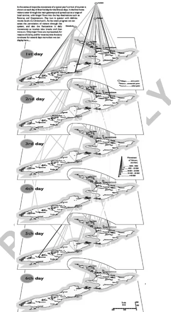
To preserve spatial information, it is appropriate to visualize aggregated transition data as Igor Drecki and Pip Forer (2000) did in their poster presentation about tourism in New Zealand. This presentation contained, among other things, the visualization shown in Figure 1, which represents the major movement flows of tourists during the first six days of their holidays in New Zealand; to summarize individual data, the travel times of different tourists have been transformed from the absolute time scale (i.e., calendar dates) to a relative one starting from the day of each tourist’s arrival in New Zealand. The diagram consists of six parallel planes, shown in a perspective view, with a map of New Zealand depicted on each plane. The planes correspond to the days of the tourists’ travel. The movements of the tourists are represented as lines connecting the locations of the major tourist destinations on successive planes. The brightness of a line corresponds to the number of people moving from its origin location (on the upper plane) to the destination location (on the lower plane) between the days corresponding to the upper and lower

planes. To make the view clearer, the authors omitted minor flows.

While this visualization has obvious advantages over a transition matrix, we are not aware of any software tools that would be able to convert movement data into such displays. As a result of the ingenious and masterly work of expert cartographers, however, the diagram and the entire poster may serve as a source of ideas and inspiration for designers of computer-based tools for the visual analysis of movement data.

Analysis and representation of movement data have long been the focus of the research work of Waldo Tobler (e.g., 1987, 2005). To visualize numbers of entities or volumes of materials that moved from one place to another, Tobler builds discrete or continuous flow maps. A discrete map represents the movements by means of bands or arrows, whose widths are proportional to the volumes moved (see Figure 2). For better legibility of such a map when the number of locations is large, minor flows may be omitted. Continuous flow maps use vector fields or stream lines to show continuous flow patterns (see Figure 3). According to Tobler, in a vector field the structure is immediately obvious, adjacent vectors being clearly correlated in length and direction. Conversely, if this is not the case, then that is also obvious. Continuous flow maps are, in principle, not limited with respect to the number of different locations present in the original data. However, producing such maps from discrete data is computationally inten-sive. This puts practical limitations to building animated flow maps or sequences of flow maps, which could represent movements during time intervals.

In the research discussed so far, aggregation helps to reduce data volume. Another approach is based on filtering: visualization is applied to a data subset selected according to a user-specified query. In this case, individual rather than aggregated data are shown. Researchers pursuing this approach focus mainly on advancing query and search techniques (Kapler and Wright 2005; Yu 2006), which are outside the scope of our study. The visualization techniques currently used are quite traditional for individual movement data: lines on a map or in a space–time cube and animation with moving icons representing the entities. It should be noted that approaches based on selection and visualization of small data subsets do not support an overall view of the collective behaviour of all entities.

data, the data need to be encoded in one of these forms. An example of using data mining for movement data is the work of Patrick Laube, Stephan Imfeld, and Robert Weibel (2005), who analyse the movements of football players during a game. Their approach is to divide the whole time into short intervals and encode the move-ments of the entities (players) during these intervals by means of symbols representing movement directions or other movement characteristics. Laube and others suggest computational methods that can search through the resulting symbol sequences for certain specific types of collective movement patterns, such as synchronous movement and ‘‘trend setting’’ (i.e., the movements of some entity are repeated by other entities after a time lag). In discussing the visualization of the New Zealand tourism data (Figure 1), we noted that the time in the data was transformed from absolute to relative: calendar dates were replaced by day numbers starting from tourists’ arrival to New Zealand. The spatial component of movement data can also undergo various transforma-tions, depending on the purposes of the analysis. Thus,

Mei-Po Kwan and Jiyeong Lee (2004) build surfaces of summary characteristics of movements not in the geographical space but in an abstract space where the dimensions are the time of day and the distance from home.

In general, not much research has been published on visualization-supported analysis of large collections of movement data. Can the existing techniques and approaches satisfy the needs of potential analysts? In order to answer this question and identify what sorts of techniques are missing (if any), we need to find out what an analyst may look for in movement data. If the major value of visualization is that it can expose patterns in data, we need to understand what types of patterns can exist in movement data. Then we will be able to determine which of the patterns types can be exposed using the existing techniques and think about appropriate methods for revealing the remaining types of patterns.

The following section looks at the structure and characteristics of movement data in order to gain a clear understanding of what is analysed. This will help us to define the types of patterns an analyst may look for in movement data.

Problem Statement

The ultimate goal of our study is to define a set of visual analytics methods to support the analysis of large collections of data about movements of multiple entities. The focus of the analysis is the collective movement behaviour of the entities rather than the behaviours of individual entities. In our search for methods, we had a special requirement: we want the methods to work even in a situation when the full data set does not fit in the computer’s memory. Hence, besides visual representation of data, the methods must involve some data-manipula-tion techniques aimed at reducing the data set to a manageable size. These may be database operations such as aggregation, sampling, and filtering or other computa-tional methods such as clustering.

Figure 3. Continuous flow maps (Tobler 1987, 2005). Reproduced by permission.

According to the functional view of a data set (Andrienko and Andrienko 2006), movement data can be treated as a function matching pairs (entity, time moment) with positions in space. This is an abstraction from real data, which have to be finite and, hence, cannot contain the position of each possible pair of entity and time. However, this abstract model is convenient and sufficient for the purpose of defining the possible tasks of data analysis and types of patterns that may exist in movement data.

From the positions of entities at different moments, other movement characteristics can be derived: speed, direction, acceleration (change of speed), turn (change of direction), and so on. We call these derivative movement characteristics.

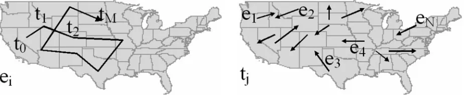
The changes in position and other movement character-istics of an entity over time form theindividual movement behaviour (IMB) of this entity (illustrated in Figure 4, left), wherebehaviouris a synoptic concept differing from the simple sequence of values of the characteristics attained at all time moments (see Andrienko and Andrienko 2006 for a more detailed explanation of the term). An IMB has its own characteristics, such as the path, or trajectory, travelled by the entity in the space; the distance travelled; the movement vector (direction from initial to final position); and the variation of speed and direction. When an analyst compares the IMBs of different entities or of the same entity at different time intervals, he or she looks for similarities and differences in terms of these synoptic characteristics.

Similarly, it is possible to look at the movement characteristics of a set of entities at some single time moment. The corresponding synoptic concept can be called the momentary collective behaviour (MCB) of this set of entities (illustrated in Figure 4, right). An MCB has such synoptic characteristics as the distribution of the entities in the space, the spatial variation of the derivative movement characteristics, and the statistical distribution of the derivative characteristics over the set of entities. These synoptic characteristics are compared when we need to find and measure similarities and differences

between MCBs at different time moments or between MCBs of different groups of entities.

The concept corresponding to a holistic view of the movement characteristics of multiple entities over a certain time period (i.e., multiple time moments) can be called dynamic collective behaviour (DCB). We assume that the DCB is the focus of interest when data about movements of multiple entities are analysed. That is, the goal of the analysis of movement data is to describe, in a parsimonious way, the DCB of all entities during the whole time period the data refer to. In addition, or in order to do this, the analyst may need to compare different DCBs: DCBs of different groups of entities during the same period, DCBs of the same group of entities during different periods, and DCBs of different entity groups during different periods.

Moreover, it is usually not sufficient just to describe the behaviour. An analyst strives to establish links between the behaviour and other potentially relevant phenomena in order to explain the behaviour or to predict how it can develop in the future. Various factors may influence movement characteristics and behaviours:

1. Properties of space

Altitude, slope, aspect, and other characteristics of the terrain

Accessibility with respect to various constraints (obstacles, availability of roads, etc.)

Character and properties of the surface (land or water, concrete or soil, forest or field, etc.) Objects present in a location (buildings, trees,

monuments, etc.)

Function or means of use (e.g., housing, shop-ping, industry, agriculture, transportation) Specific meaning of a place for a moving entity

(e.g., home, work, place for sports or for leisure) 2. Properties of time

Temporal cycles (yearly, weekly, daily, etc.) Physical characteristics: presence, intensity, and

duration of daylight

Meaning in terms of typical activities: working day vs. weekend or holiday, day vs. night

3. Properties and activities of the moving entities Individual properties: age, gender, health

condi-tion, occupacondi-tion, marital status, and so on (for people)

Way of movement (free movement, by roads, by water, by air, etc.)

Means of movement (e.g., vehicles) Purposes and/or causes of the movement Activities performed during the movement 4. Various spatial, temporal, and spatiotemporal

phenomena: climate and weather, sport and cul-tural events, legal regulations and established customs, road tolls and oil prices, shopping actions and traffic incidents, and so on.

Thus, the goals of analysing movement data referring to multiple entities may be formulated as follows: describe and compare dynamic collective behaviours and relate them to properties of space, properties of time, properties and activities of the moving entities, and relevant external phenomena. Consequently, the goal of our study is to define a set of instruments that will allow an analyst to achieve these goals.

How is the definition of the goals of analysing movement data related to the view of analysis as search for patterns? To answer this question, we need to define the notion of

pattern.

Patterns in Movement Data

As is explained in our previous work (Andrienko and Andrienko 2006), a pattern is a description or, more generally, a representation of a behaviour. A pattern may be viewed as a statement in some language (Fayyad, Piatetsky-Shapiro, and Smyth 1996). The language may be chosen quite arbitrarily (e.g., natural language, mathema-tical formulas, graphical language); therefore, the syntac-tic and morphological features of a pattern are irrelevant to data analysis. What is relevant is the meaning, or semantics. It is natural to assume that representations of the same behaviour in different languages have a common meaning. Hence, the constructs of the different languages refer to the same system of basic language-independent elements, from which various meanings can be composed. By analogy with meanings of words in a natural language, we can posit that the basic semantic elements for building various patterns include generalpattern typesandpattern properties. A specific pattern is aninstantiationof one or more pattern types. This is analogous to the specialization of a general notion by means of appropriate qualifiers. In the case of patterns, the qualifiers are specific values of the pattern properties. For example, the pattern ‘‘entities e1,

e2,. . ., en moved together during the time period T’’

instantiates the pattern type ‘‘joint movement’’ by specifying what entities and when moved in this manner.

It is quite reasonable to assume that general pattern types exist in the mind of a data analyst as mental schemata. Moreover, it is quite likely that these schemata drive the process of visual data analysis, which is commonly believed to be based on pattern recognition: the analyst looks for constructs that can be associated with known pattern types. Once such a construct is detected, the analyst observes and measures the values of the pattern properties. Visual analytics methods should be designed so as to facilitate the detection of instances of the possible pattern types. Therefore, in order to design proper visual analytics methods for movement data, we must first define the pattern types relevant to such data.

For this purpose, let us have a closer look at what we call

dynamic collective behaviour, or DCB. A DCB can be viewed from two different perspectives:

As a construct formed from the IMBs of all entities (i.e., the behaviour of the IMB over the set of entities)

As a construct formed from the MCBs at all time moments (i.e., the behaviour of the MCB over time) These two views are called aspectual behaviours (a term introduced in Andrienko and Andrienko 2006). Aspectual behaviours exist in multidimensional data (i.e., data having two or more referential components, or indepen-dent variables). Movement data have two referential components, entity and time (recall the abstract model of movement data introduced in the previous section), which yield two aspectual behaviours. The aspectual behaviours are essentially different and must be described in terms of different types of patterns.

Our previous work (Andrienko and Andrienko 2006) introduces the basic (most general) types of patterns: similarity, difference, arrangement, and summary. Here, we specialize these basic types for movement data. We omit the type ‘‘summary,’’ which corresponds to the summarization of multiple characteristics by means of statistics or other computational methods, and focus on pattern types whose instances can be detected visually. The behaviour of the IMB over the set of entities can be described by means of similarity and difference patterns, that is, as groups of entities having similar IMBs that differ from the IMBs of other groups of entities. It may happen that some entities have quite peculiar IMBs that differ from the IMBs of all other entities. Such peculiar IMBs are also described by means of difference patterns. Arrangement patterns are not relevant to the behaviour of the IMB over the set of entities because the set of entities has no natural ordering and no distances between the elements (see Andrienko and Andrienko 2006).

them are relevant:

1. Similarity of overall characteristics (geometric shapes of the trajectories, travelled distances, durations, movement vectors, etc.)

2. Co-location in space (i.e., the trajectories of the entities consist of the same positions or have some positions in common):

ordered co-location: the common positions are attained in the same order

order-irrelevant co-location: the common posi-tions may be attained in different orders symmetry: the common positions are attained in

opposite orders 3. Synchronization in time:

Full synchronization: similar changes of move-ment characteristics occur at the same times Lagged synchronization: changes of the

move-ment characteristics of entity e1 are similar to

changes of the movement characteristics of entity e0but occur after a time delay t

4. Co-incidence in space and time:

Full co-incidence: the same positions are attained at the same time

Lagged co-incidence: entity e1 attains the same

positions as entity e0but after a time delay t

All these types of similarity are possible specializations of the general notion of a similarity pattern.

Let us now consider the other aspectual behaviour, that is, the behaviour of the MCB over time. Mathematically, time is a continuous set where ordering and distances exist between the elements (i.e., time moments). Hence, besides similarity and difference patterns, arrangement patterns are relevant. An arrangement pattern describes changes in the MCB with respect to the ordering and distances between the corresponding time moments – for example, an increase in the number of entities in some part of the space and a decrease in other parts. Here are the pattern types for describing the behaviour of the MCB over time (we note in parentheses the basic pattern types that have been specialized):

1. Constancy (similarity): the MCB is the same or changes insignificantly during a time interval 2. Change (difference): the MCB changes significantly

from moment t1 to moment t2

3. Trend (arrangement): consistent changes in the MCB during a time interval

4. Fluctuation (arrangement): irregular changes in the MCB during an interval

5. Pattern change or pattern difference (difference): the behaviour of the MCB during time interval T1

differs from that during time interval T2. The term

‘‘pattern change’’ applies when T1 and T2 are

adjacent. For example, a trend can change for

constancy or for a different trend. The term ‘‘pattern difference’’ applies to non-adjacent time intervals.

6. Repetition (similarity): occurrences of the same patterns of types 1, 3, or 4 or the same pattern sequences at different time intervals

7. Periodicity, or regular repetition (similarity and arrangement): occurrence of the same patterns or pattern sequences at regularly spaced time intervals 8. Symmetry (similarity and arrangement): opposite trends or pattern sequences where the same patterns are arranged in opposite orders

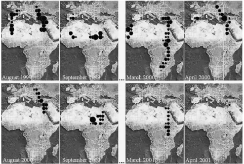
The pattern types listed above can be called ‘‘descriptive,’’ since they can be used to describe a DCB. Behaviours corresponding to some of these pattern types can be seen in the visualization partly reproduced in Figure 5. The visualization represents the movements of a number of white storks during two migration seasons: more specifically, movement speeds aggregated temporally by months and spatially by cells of a regular grid. The upper left map demonstrates similarities and differences between IMBs. There are two groups of birds with different IMBs: some birds fly on the west, while the other group flies on the east. An ordered spatial co-location exists between the movements of the birds in each group. The sequence of maps in each row demonstrates changes in the MCB over time. Moreover, there are vivid trends: consistent shifts in the positions of the birds to the south at the beginning of the migration season and to the north at the end of the season. A symmetry pattern can be seen between the southward movement trend in August and September and the northward movement trend in March and April. Comparison of the migration movements in different seasons reveals periodicity patterns, despite the presence of certain difference patterns between the seasons. Unfortunately, Figure 5 provides very limited possibilities for comparisons, as it includes, for space saving reasons, maps for four only selected months in two selected seasons.

Relations between the DCB and properties of space, time, entities, external phenomena, and events need to be described in terms of different types of patterns: correlation, influence, and structure (Andrienko and Andrienko 2006). We use the term ‘‘correlation’’ in a more general sense than statistical correlation between numeric variables; it may also denote co-occurrence of any characteristics, in particular spatial and qualitative, and co-occurrence of behavioural patterns. Influence

Correlation, influence, and structure are collectively called

connectional patterns.

To analyse movement data, an analyst needs tools and methods that facilitate the discovery of all types of patterns, both descriptive and connectional. However, the design of such tools and methods faces a number of challenges that can be quite difficult to overcome.

Challenges

Irrespective of the size of a data set, movement data are difficult to visualize and analyse because of the quite complex data structure, which involves time, space, multiple entities, and multiple movement characteristics. Is there any way to display all this information so that the representation is comprehensible to a human viewer? The representation of two-dimensional space requires two display dimensions. Time may be represented by means of the third spatial dimension, as in a space–time cube, also called a space–time aquarium (Ha¨gerstrand 1970; Kraak 2003), or by means of the temporal dimension in an animated display (Andrienko, Andrienko, and Gatalsky

2000, 2005). There are also other ways of representing time in combination with space (Vasiliev 1997), but they are much more limited with respect to the number of different values that can be discernibly shown in a display. From a representation of individual trajectories by means of lines in an interactive 3D display, it is possible to estimate the positions, speeds, directions, and other movement characteristics at different times. Similarities and differences between IMBs are noticeable. The use of a movable plane, as suggested by Menno-Jan Kraak (2003), helps in exploring the MCBs at different moments and the behaviour of the MCB over time. However, all these benefits fade away with an increase in the number of moving entities, the length of the time period, or the geometric complexity of the trajectories. The data do not need to be very numerous: a space–time cube with only 10 trajectories will already look like a bowl of spaghetti, from which one can extract hardly any useful informa-tion. Similarly, an animated display of individual move-ments (in particular, the ‘‘time window’’ mode of animation as described by Andrienko and others 2000, 2005) is quite appropriate when the entities are few and

the time period not very long but decreases in utility with increasing numbers of moving entities or time moments in the data. The upper limit may be higher for an animated display than for a space–time cube: in an animated display, the information is presented in portions, which makes the display at any given moment simpler and easier to perceive than a space–time cube, which portrays all information at once. However, this slight increase in the applicability limit does not solve the problem in general. Besides, the portion-wise representa-tion of informarepresenta-tion has clear disadvantages: no overview of the whole data set is possible, nor is any comparison between states at different moments.

Data-size limitations on visual displays arise long before the size becomes too big for the computer’s memory. Therefore, some methods for reducing the size of the data set must be applied prior to the visualization. Possible approaches include aggregation, filtering, and clustering. When the data set is too big for human perception but not yet too big for the computer, high interactivity may compensate for the inevitable information losses resulting from data reduction. Suppose, for example, that the visualization shown in Figure 1 is an interactive display on the computer screen that allows the user to click on the lines in order to select the corresponding entities. In response, the movements of the selected entities are shown in the display as lines of a different colour. Through further interaction with the display, the user may modify the selection and immediately receive visual feedback. Moreover, several displays of aggregated data providing complementary views of the data set may be linked by means of brushing, similarly to the linked histograms in Attribute Explorer (Spence and Tweedy 1998; Spence 2001). For example, the display with tiered maps, as in Figure 1, may be linked to a bar chart showing the numbers of tourists coming from different countries. When the user selects a subset of tourists through the tiered map display, the bar chart shows how many of these tourists come from each country by means of special colouring of the corresponding bar segments. The user may also select the tourists coming from a particular country by clicking on the respective bar chart. In response, the tiered map display will show the flows of these tourists.

Things become much more complicated when the original data cannot be stored and processed in the computer’s memory. This means that aggregation, filter-ing, clusterfilter-ing, selection, and brushing cannot be done without the involvement of database operations, which may take a great deal of time. Hence, the visual displays can no longer be interactive in the same way as with smaller data sets. It is necessary to devise new methods of interaction that can still perform reasonably well when data sets are huge.

Because of the challenges arising from large data volumes, Daniel Keim (2005) argues that Ben Shneiderman’s Information Seeking Mantra – ‘‘Overview first, zoom and filter, and then details-on-demand’’ (1996) – should be replaced by a Visual Analytics Mantra (VAM): ‘‘Analyse First – Show the Important – Zoom, Filter and Analyse Further – Details on Demand.’’ The VAM stresses the fact that fully visual and interactive methods do not work with large data sets. It is necessary to start with database operations and computations (‘‘Analyse1First’’) and apply visualization to the results obtained (‘‘Show the Important’’). The user may interact with the visualization and the secondary data it represents (i.e., the outcomes of the analysis but not the original data), in particular by zooming and filtering, and may trigger further analysis, which, again, requires visualization of the results. In this way, visual analytics is an iterative process involving three major steps: computational analysis, visualization of the results of the computational analysis, and interactive visual analysis of these results. A detailed consideration (‘‘Details on Demand’’) is possible for small data portions when they require, for some reason, special attention from the analyst. This does not necessarily happen at the end of the process.

Thus, visual analytics tools for movement data need to be designed in accord with the VAM, whereby database technologies and computational analysis are applied prior to visualization and iteratively reapplied during the process of data analysis. Let us now examine what methods for data manipulation, computational analysis, visualization, and interaction might be suitable to support the analyst in detecting the diverse types of patterns in massive movement data.

Supporting Pattern Detection: A Road Map

DATA MANIPULATION

Aggregation

collective movement patterns on weekdays and weekends, and so on.

Hence, the appropriate degree of data aggregation and generalization is not determined simply by finding a good trade-off between the simplification gained and the amount of information lost. The aggregation must be adequate to the goals of the analysis (i.e., the scale at which the analyst seeks to detect patterns). If the interests of the analyst include patterns at different scales, it is necessary to consider the data at different levels of aggregation. Tools for visual analysis must therefore enable the user to do this.

Aggregation consists of two operations: (1) grouping individual data items (i.e., dividing the data into subsets); and (2) deriving characteristics of the subsets from the individual characteristics of their members. Typically, various statistical summaries are used as characteristics of the subsets: number of elements, mean, median, mini-mum, maximum values of characteristics, mode, percen-tiles, and so on. It is also important to know the degree of variation of the characteristics within the aggregates. For this purposes, such statistical measures as variance (or standard deviation) or inter-quartile distance are com-puted. Aggregates with high variation of characteristics among members should not be used in data analysis, since they may lead the analyst to incorrect conclusions about the data.

Methods for grouping/dividing movement data

Grouping/division may be necessary not only for data aggregation but also for other kinds of data processing, such as clustering. Movement data involve two referential components: the set of entities and the time. Grouping/ division may be applied to either or both. The time may be divided into equal-length intervals (e.g., 10 minutes, one hour, one week); depending on the data and analysis goals, it may also be useful to divide the time into slightly unequal intervals corresponding to calendar units, such as months, quarters, or years, or to apply other division principles (e.g., to divide a school year into semesters and breaks). Furthermore, it may be reasonable to divide the time into subsets consisting of non-contiguous intervals, in particular, according to one or more of the temporal cycles; the user may wish to group all Mondays, all Tuesdays, and so on. Hence, the data analytics toolkit should include a tool for time partitioning whereby the user can flexibly define the principles of division. A similar tool is needed for dividing the set of entities. This set has no distances that can provide a basis for division, as in the case of time. It can instead be divided on the basis of the characteristics of the entities (e.g., age or occupation, in the case of people) or characteristics of their movement (e.g., position in space, speed, direction). This means that entities with similar values for the selected characteristics are grouped together. For the

purposes of this grouping, either computational methods (clustering) or interactive techniques can be applied. The groups (clusters) of entities resulting from computational methods may be quite difficult to interpret. An appro-priate visualization of the characteristics of the entities forming the clusters may be helpful.

For interactive grouping, the user chooses the character-istics and specifies equivalence classes between their values (i.e., which values must be treated as similar). The method of defining equivalence classes depends on the type of a characteristic. Thus, for numeric values, the user divides the whole value range into intervals. If the values of a qualitative characteristic are not too numerous, groups are formed from entities with equal values; otherwise, the user may wish to divide the values into classes according to their semantic closeness. For positions in space, the user may divide the space into compartments. In particular, these may be cells of a regular grid, with the cell size and, possibly, shape (e.g., rectangular or hexagonal) chosen by the user. These may also be units of an administrative or other existing territorial division or regions specified interactively according to any appropriate criteria such as surface type, way of use, accessibility, or other relevant properties of the space (see the list given under ‘‘Problem Statement’’ above). The visual analytics tools should support such arbitrary divisions of the space. Thus, the user may define space compartments by interacting with a map display or by applying database search operations such as retrieving the locations of schools, shops, and so on.

As mentioned above, entities may be grouped according to values of their movement characteristics. Since these values change over time, interactive grouping can be carried out on the basis of values at selected moments or on the basis of aggregated values over time intervals. Unfortunately, selection of each additional time moment or interval multiplies the number of groups and causes difficulties for the visualization and visual exploration of the results of the aggregation.

Besides values at selected moments, entities can also be grouped on the basis of changesin the values occurring between two moments in time. A change involves several aspects:

the original value and the resulting value

the amount or degree of change, that is, the absolute or relative distance between the original and resulting values (in a case when distances between the values exist)

the direction of change: increase or decrease for numeric or ordinal values; spatial direction for positions

aggregate entities according to changes in their speed from moment txto moment ty. The user may divide the

whole range of speeds into intervals (say, three intervals: low, medium, and high speed) and build aggregates on the basis of all possible pairs (i.e., low/low, low/medium, low/high, medium/low, etc.). The user may also find the range of speed change, that is, from the maximum decrease (taken as a negative number) to the maximum increase, and aggregate the entities by dividing this range into suitable intervals. Or, again, user may divide the entities into three groups depending on whether their speed has increased, decreased, or remained the same. It is clear that these approaches to aggregation are not equivalent in terms of the information that may be gained as a result. By analogy to the example of speed, grouping the entities according to changes in their spatial position may be done on the basis of possible pairs composed of a source position and a destination position, on the basis of the distances between original and final positions, or on the basis of the spatial direction in which the destination lies with respect to the source position. Methods for dividing (grouping) movement data are summarized in Table 1.

Change computation: Transformations of space and time

Aggregation is not the only useful data transformation, and we shall briefly discuss some other data-manipulation techniques that may increase the comprehensiveness of

analysis and give additional insights into the data. One of them is the computation of the amount or degree and the direction of change, which is valuable not only for grouping of the entities by also in itself. Thus, it may be useful to look at change maps portraying (in a generalized manner) changes in MCB from one moment to another. Among the possible methods, the most useful may be transformations of space and time from absolute to relative. Similarities between temporally or spatially separated behaviours can more easily be detected when these behaviours are somehow aligned in time or in space. To align behaviours in time, the ‘‘objective,’’ absolute time of each behaviour (i.e., calendar date and time) is ignored and only its ‘‘internal’’ time is considered (i.e., the time relative to the moment when this behaviour began). An example is the representation of tourist movements in New Zealand (Figure 1). The tourists come to New Zealand on different days; however, the data are presented as though all the tourists arrived simulta-neously. For this purpose, the designers of the visualiza-tion transformed the absolute dates into day numbers starting from the day of arrival to New Zealand.

In this example, the analysts superposed the starting times of the IMBs of different tourists. It may also be useful to superpose both starting and ending times. In this case, the absolute time moments in each IMB are transformed into their distances from the starting moment and divided by the duration of the behaviours (i.e., the lengths of the

Table 1 Methods of dividing/grouping movement data

What Is Divided/Division Principle Method of Division Examples

Time / inherent ordering and distances Regular intervals 10 minutes, 2 hours

Existing division Days, months

Temporal cycles Time of day, day of week

‘‘Semantic’’ division Day and night; workday and weekend Entities / numeric characteristics Regular intervals Speed: 0–10, 10–20,. . ., 190–200 km/hour

‘‘Semantic’’ intervals Age: 0–15, 16–24, 25–64, 65þ

Entities / qualitative characteristics Individual values Vehicle type: bike, motorbike, car, truck

‘‘Semantic’’ groups of values Travel purpose: business (work, study), shopping and services, leisure (sports, walk,

entertainment)

Entities / spatial positions Regular sections Rectangular grid

Existing division Administrative districts, cities Space properties Water, forest, field, built-up area

‘‘Semantic’’ division City centre, residential area, shopping area, industrial area

Entities / changes Original and resulting values From France to Germany, from Germany to

France, from France to the United Kingdom, from the United Kingdom to France (see Figure 2)

Amount or degree of change Distance travelled: 0–0.01 km (no change), 0.01– 100 km, 100–500 km

intervals between the starting and ending moments). This facilitates the detection of similarities between movements performed at different speeds. Such an approach could be useful, for example, in comparing the movements of migratory animals in different years.

Moreover, there may be cases when non-uniform transformation of the time of each IMB is reasonable. For example, an analyst exploring the daily movements of people may be interested in excluding the times when these people stay in the same place for an extended period (e.g., at work, in a shop, at home) and adjusting the times when they move. In this case, time transformation is performed separately for each interval of movement. Analogous ideas can be applied for spatial alignment of IMBs initially disjoint in space. An analyst may try to bring a set of IMBs (trajectories) to a common origin and search for coincidences between them. Furthermore, the analyst may be interested in disregarding the direction of movement and considering only changes in direction (turns). For this purpose, the trajectories are ‘‘rotated’’ until the initial movement directions coincide. Coincidences between further trajectory fragments indi-cate similarities. It may also be useful to ‘‘stretch’’ or ‘‘shrink’’ the trajectories to adjust their lengths.

In looking for co-location of trajectories where positions are specified as points in space, it may be reasonable to apply a kind of ‘‘spatial coarsening,’’ that is, to replace the original points with regions (areas), for example, circles with some chosen radius around the points. The resulting trajectories are treated as similar when there is an overlap between their ‘‘expanded’’ positions, even though there may be no sharp co-incidence between the original positions.

In studying MCBs and their behaviours over time, it may be appropriate to treat the space as a discrete set of coarsely defined ‘‘places’’ rather than as a continuous set consisting of dimensionless points. For this purpose, one uses space partitioning, which has been discussed before in relation to data aggregation. Such a transformation may be called ‘‘space discretization.’’ Furthermore, it may be useful to transform the geographical space into a kind of ‘‘semantic’’ space consisting of such locations as home, workplace, shopping site, and sport facility. Each trajectory is then transformed into a sequence of move-ments between pairs of these locations, and the analyst looks for similar sub-sequences occurring in different trajectories.

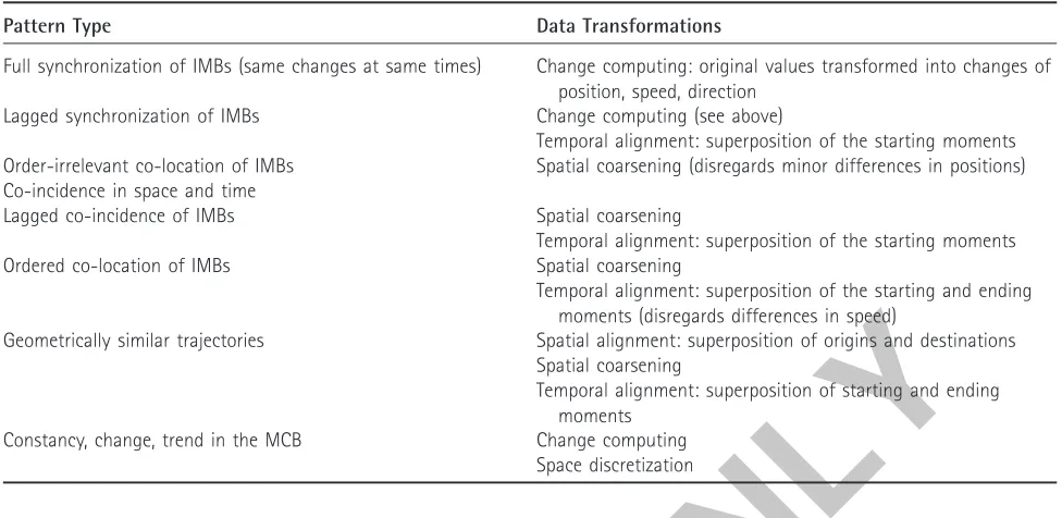
Table 2 indicates what types of patterns various data transformations may help to detect.

When we say that the analyst looks for similarities between IMBs, we do not really mean that the IMBs are presented to the analyst as individual items, without aggregation or generalization. As discussed above, the large size of the data set precludes this method of analysis. Therefore, similarities between IMBs need to be detected somehow without the analyst’s seeing the IMBs. This can only be done by using methods of computational analysis, as discussed in the next subsection.

EXPLORING THE BEHAVIOUR OF IMBS OVER THE SET OF ENTITIES

Clustering of IMBs

In order to analyse IMBs without seeing them, the analyst can apply clustering methods, which divide entities into groups so that the entities within each group are as similar as possible and differ as much as possible from the entities

Table 2 Some types of patterns in movement data and data transformations that may support pattern detection

Pattern Type Data Transformations

Full synchronization of IMBs (same changes at same times) Change computing: original values transformed into changes of position, speed, direction

Lagged synchronization of IMBs Change computing (see above)

Temporal alignment: superposition of the starting moments Order-irrelevant co-location of IMBs Spatial coarsening (disregards minor differences in positions) Co-incidence in space and time

Lagged co-incidence of IMBs Spatial coarsening

Temporal alignment: superposition of the starting moments

Ordered co-location of IMBs Spatial coarsening

Temporal alignment: superposition of the starting and ending moments (disregards differences in speed)

Geometrically similar trajectories Spatial alignment: superposition of origins and destinations Spatial coarsening

Temporal alignment: superposition of starting and ending moments

Constancy, change, trend in the MCB Change computing

in the other groups. If a clustering method can group the moving entities according to similarities and differences in their IMBs, the analyst can then look at various aggregated characteristics and aggregated behaviours of the groups instead of looking at the individual behaviours. A clustering method computes numeric values expressing the degree of similarity between entities. These values are usually called ‘‘distances’’ (in an abstract sense): the smaller the distance, the more similarity exists between the entities. Thus, to group moving entities according to their IMBs, it is necessary to find a way to express numerically the degree of similarity between two IMBs, or, in other words, to define a method for computing distances between IMBs. Such a method will be referred to here as a ‘‘distance function.’’

As we have noted, two or more IMBs may be similar in various diverse ways, and any type of similarity may be of interest. Each type of similarity requires a different distance function. Thus, the degree of spatial and temporal co-incidence is computed from the distances between the spatial positions at the corresponding moments. The same function would be suitable for lagged co-incidence after applying temporal alignment to the IMBs (see Table 2). The degree of order-irrelevant co-location may be computed from the distances between each position on one trajectory and the nearest position on the other trajectory. For the degree of ordered co-location, the corresponding function must find common (overlapping) positions and check whether they were reached in the same order. This method is also suitable for estimating the degree of similarity of trajectory shapes after the trajectories have been spatially aligned.

Hence, it is reasonable to devise a clustering tool where the distance function is replaceable. In this case, the analyst could choose the appropriate distance function, depending on his or her current interests, and let the clustering tool run with the use of this function. A library of appropriate distance functions can be created in advance, as well as a library of data-transformation methods.

It should be also borne in mind that the existence and the types of similarity patterns between IMBs depend on the temporal resolution chosen for looking at the data. Thus, fine movements of entities, which are made at the scale of minutes or hours, may be quite different, yet there may be a clear similarity between the behaviours of the same entities considered at the scale of days or weeks. It makes sense, therefore, to run a clustering method several times with the same distance function but different degrees of aggregation and generalization of the data with respect to time (i.e., with the time partitioned into intervals of different lengths).

A serious technical problem in applying clustering algorithms is that they can work effectively only when

the data are resident in computer memory. The reason for this is the necessity for numerous and repeated distance computations. Not only do pair-wise distances between entities need to be computed but also, as clusters are built, the distances between the current clusters (which change over time) and those entities that have not yet been attached to any cluster must be computed as well. When the data set is too big for the computer’s memory, clustering may require too much time.

One possible way to cope with this problem is based on sampling. The idea is that a subset of entities is sampled from the whole set of entities so that the corresponding movement data set is of a size suitable for effective clustering. Depending on the specifics of the data and the goals of the analysis, it may also be reasonable to sample fragments of IMBs. For example, from data about people’s movements over many days, fragments corresponding to one-day movements of individuals can be sampled. Once a manageable subset of IMBs or fragments of IMBs has been extracted, clustering is applied to this subset. After the clusters are built, the distances between them and each of the remaining IMBs or fragments can be computed, using the same distance function as for the clustering. This requires a single run through the database. On this basis, each IMB or fragment is attached to the closest cluster or, if it is too distant from all clusters, selected for further application of clustering or for detailed consideration by the user (this may be an anomalous behaviour).

Visualization of clustering results

Thus, when IMBs have been clustered on the basis of the co-location of trajectories, a suitable visualization would be a map which, for each location in space (real space or, if there are too many locations in the source data, the results of space discretization), shows how many trajec-tories it appears in. Graduated symbols or graduated shading would be suitable for this purpose. A separate map is built for each cluster, which enables comparison of the clusters.

For ordered location and for spatiotemporal co-incidence, it is reasonable to compute, for each pair of locationsxandy and time intervalT, how many cluster members moved fromxtoyduring the intervalT, where

T results from an appropriate partitioning of the time (which may be previously transformed, as discussed in the previous section). A good way to visualize such statistics is using tiered maps, as in Figure 1. In the case of ordered co-location, the third (temporal) dimension reflects the temporal order; in the case of spatiotemporal co-incidence, either full or lagged, the third dimension also reflects temporal distances.

Another possible way to visualize results of clustering is to portray the individual trajectories, possibly transformed, if data transformation has been used for the clustering operation. Since the trajectories are supposed to be close and similar, the resulting display is less likely to resemble a bowl of spaghetti and may be quite comprehensible. If the trajectories are represented by semi-transparent lines, darker shades will emerge where many lines overlap, in this way indicating the common features of the trajec-tories. However, this idea needs to be verified by implementing and testing both clustering methods and visualization.

When clustering is used to group IMBs according to derivative movement characteristics rather than positions, other types of visualization are appropriate. For example, variation in speed may be shown on a time graph, while a segmented bar chart might represent the distribution of movement directions at each time moment.

Besides the features of the IMBs of cluster members, the analyst should be informed about the number of members in each cluster and the statistics of their static character-istics, if these are available in the data. The analyst should also be able to obtain any statistics concerning the movement of the entities, such as average and maximal speed or total distance travelled.

Apart from computational clustering and visual examina-tion of the results, the user may be interested in a close look at subsets of IMBs with specific features (e.g., the trajectories whereby entities move toward the city centre in the morning and away from the city centre in the evening). For this purpose, interactive query tools are necessary. A challenge is to design effective methods for data retrieval and visualization to ensure an acceptable

reaction time. It is also important to design a proper user interface, taking into account that quite perceptible delays are unavoidable with large data sets, especially when the data are not memory resident. Thus, the principle of the dynamic query (Ahlberg, Williamson, and Shneiderman 1992), whereby the tool immediately reacts to any slight user interaction with the query device, such as moving a slider by one pixel, is not applicable to this case. However, the tool should enable the user to work by refining the query interatively, depending on the results of the previous stage, as well as by formulating a complete query all at once.

EXPLORING THE BEHAVIOUR OF THE MCB OVER TIME

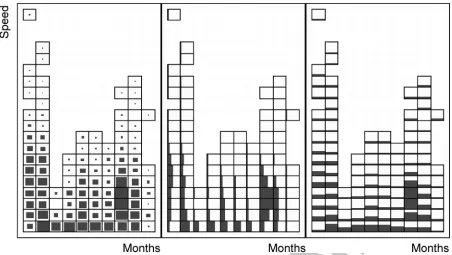
In order to explore the behaviour of the MCB over time, the analyst needs visualizations that show him or her the MCB at different time moments or, in a summarized way, at different intervals into which the whole time of movement is divided. There are two basic ways to do this: an animated display (map, diagram, or graph, depending on the information to be portrayed) and multiple uniform displays, or ‘‘small multiples,’’ in the terms of E.R. Tufte (1983; see illustration in Figure 5). We will not discuss here the advantages and disadvantages of each approach (in our opinion, they are complementary and should be used in combination); instead we will focus on the content of a single animation frame or a single display in small multiples, which corresponds to the MCB at a single time moment or during a single interval. In order to look at the spatial distribution of the moving entities at a selected time moment (interval), it is natural to use a map. Since the entities are very numerous, their positions must be shown in an aggregated manner (i.e., as densities). Some approaches visualize densities as smooth surfaces, built using kernel methods or other computa-tional techniques. Such surfaces are represented by colouring or shading, by contour lines (isolines), or in 3D views, which are rather appealing visually. Another approach is ‘‘binned’’ visualization of densities, whereby the map area is divided into regular ‘‘bins’’ or cells (e.g., squares) and the number of entities fitting into each cell is shown by colouring, shading, or graduated symbols (see Figures 5 and 6). Such a visualization can be built using database operations. The user can vary the size of a cell in order to look at the data at different levels of aggregation (of course, re-aggregation of a large database may require some time).

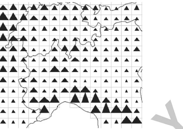
each cell, such as average, minimum, and maximum speeds or the number of entities moving in each direction. A single value (such as average speed) may be represented by colouring, shading, or graduated symbols, as in Figures 5 and 6. Prevailing movement directions can be indicated by arrows, as in Figure 3 (left). Several values (e.g., numbers of entities moving in different directions) require the use of diagrams. The sizes of the diagrams should not exceed the sizes of the cells where they are placed, and therefore the cells must be large enough for the diagrams to be legible. Representations of average, median, or most frequent values should be accompanied by the display of appropriate statistics expressing the degree of variance. An example is given in Figure 7, where triangle symbols are used to represent both the mean values and the variances of the values in the cells. As a complement to maps and perspective views of the (geographical) space, non-cartographic displays are used to look at the statistical distribution of various movement characteristics at different time moments or over different intervals. Frequency histograms provide aggregated infor-mation about the statistical distribution of numeric values; statistics about qualitative values can be shown

by bar charts in which each bar corresponds to one value and the size of the bar is proportional to the number of occurrences of this value. For statistics about movements in different directions, it may be convenient to use radial bar charts, wherein the orientation of the bars corre-sponds to spatial directions: north, north-east, east, and so on. By analogy to the spatial views, such displays are built for each moment (interval) in time and presented simultaneously as small multiples or in temporal sequence (animation).

Another possibility is to represent the time using one of the display dimensions, as in a time graph. For example, this might be a display wherein the horizontal dimension represents the whole time period divided into intervals; for each interval there is a segmented bar showing the frequencies of different values of some movement characteristic, that is, the number of occurrences of each value (for qualitative values) or the number of occur-rences of values from each of the intervals previously specified by the user (for numeric values).

To facilitate detection of significant changes in the MCB, it is useful to compute and visualize the changes that take place from one moment (interval) to another, in

particular, changes with respect to the previous moment or interval. For example, with ‘‘binned’’ maps, the differences between the values in the cells at consecutive moments (intervals) may be computed and represented by cell colouring. It is reasonable to use a diverging colour scale (Brewer 1994) on which one hue represents decrease and another represents increase. It is also useful to compute changes in the movement characteristics of the individual entities and represent them in an aggregated way on maps and non-cartographic displays. For example, the visualization technique using temporally ordered segmented bars, discussed above, may be used to represent changes in speed: how many entities decreased their speed (by more thanx%, by x1 to x2%, etc.), how

many entities kept the same speed, and how many entities increased their speed (by more than x%, by x1 to x2%,

etc.). While the primary focus of the analysis is the collective movement behaviour rather than individual movements, significant changes in the statistical or spatial distribution of individual movement characteristics may indicate changes in collective behaviour.

It should be noted that aggregated displays can be used not only for viewing the data but also as direct manipulation query devices: the user can select subsets of data by selecting the aggregates representing them (e.g., cells on a map, bars in a histogram, or segments in segmented bars). To support such interaction, the displays must ‘‘remember’’ how each aggregate has been produced and be able to transform user actions into appropriate database queries. However, it must be taken into account that noticeable time may be needed to fulfil queries in the case of massive data sets. Therefore, immediate reaction of the tool to any user click or slight mouse movement may be inappropriate. Instead, the user should be able to make

and modify selections without triggering any queries and, when the selection process is finished, to signify this explicitly.

LOOKING FOR CONNECTIONAL PATTERNS

Interactive techniques

Direct-manipulation query interfaces are especially con-venient for brushing, where the user interactively selects a subset of data and, in response, graphical elements in different displays corresponding to this subset are similarly marked (highlighted). Brushing helps the analyst to establish links between two or more displays providing complementary information. This, in turn, may be helpful in a search for connectional patterns (i.e., correlations, influences, and structural links between characteristics, phenomena, processes, events, etc.).

For example, the analyst may use a map to select areas with a high density of moving entities at some time momentt1. From maps corresponding to other moments,

the analyst will learn whether the densities are always higher in these areas than in the remaining territory, which may indicate a link between the number of moving entities and the properties of the space where they move. From speed histograms, the analyst may see whether there is any relation between the areas of high density and the variation of the speed of movement, such as high speeds of the entities before entering the areas of high density, low speeds inside these areas, and high speeds after exiting these areas. Furthermore, simultaneously with the displays of the movement data, the statistical distribution of the static properties of the moving entities or their activities, by time intervals, may be visualized. Then the analyst can discern whether the entities in the areas of high density