Supply chain risk network management : a bayesian belief network and expected utility based approach for managing supply chain risks

Supply Chain Risk Network Management: A Bayesian Belief Network and

Expected Utility Based Approach for Managing Supply Chain Risks

Abroon Qazia,∗, Alex Dicksonb, John Quigleya, Barbara Gaudenzic

a_{Department of Management Science, University of Strathclyde, William Duncan Building, 130 Rottenrow, Glasgow, G4}

0GE, Scotland

b_{Department of Economics, University of Strathclyde, William Duncan Building, 130 Rottenrow, Glasgow, G4 0GE,}

Scotland c

Department of Business Administration, University of Verona, Via Cantarane 24, Verona, Italy

∗

Corresponding author

Email addresses: [email protected](Abroon Qazi),[email protected](Alex Dickson),

[email protected](John Quigley),[email protected](Barbara Gaudenzi)

*Title page including author details

Bayesian Belief Networks Expected Utility Theory

Safety and Reliability Engineering Multi-Criteria Decision Analysis

Risk Identification

Risk Analysis and Evaluation

Risk Treatment 𝐸𝑈

Context specification

Optimisation 𝑅𝑃𝑀

Critical risks Risk

Re-assessment

𝑇𝑖𝑚𝑒: 𝑇 = 𝑡0 Fault Tree

Analysis

𝑇𝑖𝑚𝑒: 𝑇 > 𝑡0 Risk

Monitoring 𝑊𝑁𝐸 Risk Appetite

Swing Weights

Risk and Performance

Network

Modified Risk Matrix

Optimal strategies

Highlights

• A SCRM process integrating all stages of the risk management process is proposed and opera-tionalised.

• The operationalisation scheme adapts and integrates various techniques from diversified research areas.

• ‘Probability-conditional expected utility’ matrix is introduced to assess interdependent risks.

• ‘Weighted net evaluation of risk mitigation’ is proposed to capture the decision maker’s risk appetite.

• Propositions are introduced to elucidate the significance of modelling interdependent risks.

1 2 3 4 5 6 7 8 9 10 11 12 13 14 15 16 17 18 19 20 21 22 23 24 25 26 27 28 29 30 31 32 33 34 35 36 37 38 39 40 41 42 43 44 45 46 47 48 49 50 51 52 53 54 55 56 57 58 59 60 61 62 63

Supply Chain Risk Network Management: A Bayesian Belief Network and

Expected Utility Based Approach for Managing Supply Chain Risks

Abstract

The paper develops and operationalises a supply chain risk network management (SCRNM) process that captures interdependencies between risks, multiple (potentially conflicting) performance measures and risk mitigation strategies within a (risk) network setting. The process helps in prioritising risks and strategies specific to the decision maker’s risk appetite. The process is demonstrated through a case study conducted in a global manufacturing supply chain involving semi-structured interviews and focus group sessions with experts in risk management. Theoretically grounded in the framework of Bayesian Belief Networks (BBNs) and Expected Utility Theory (EUT), the modelling approach has a number of distinctive characteristics. It utilises a top-down approach of Fault Tree Analysis (FTA). Performance measures are identified first and subsequently connected to risks. A ‘probability-conditional expected utility’ matrix is introduced to reflect the propagation impact of interdependent risks on all performance measures identified. A ‘weighted net evaluation of risk mitigation’ method is proposed and the method of ‘swing weights’ is used to capture the trade-off between the efficacy of strategies and the associated cost keeping in view the decision maker’s risk appetite. The approach adapts and integrates techniques from safety and reliability engineering (FTA), decision making under uncertainty (EUT), and multi-criteria decision analysis (swing weights). The merits and challenges associated with the implementation of interdependency based frameworks are discussed. Propositions are presented to elucidate the significance of modelling interdependency between risks and strategies.

Keywords: Supply Chain Risk Network Management, Interdependencies, Multiple Performance Mea-sures, Risk Mitigation Strategies, Bayesian Belief Networks, Expected Utility.

1. Introduction

Aiming for competitive advantage, firms operating across the global marketplace are exposed to considerable risk (Tang & Tomlin, 2008; Christopher et al., 2011; Blos & Miyagi, 2015). The com-mencement of research in supply chain risk management (SCRM) dates back to the early years of 21stcentury (Harland et al., 2003; Christopher & Peck, 2004; Manuj & Mentzer, 2008). There is an extensive literature on SCRM that considers conceptual theory building facets as well as empirical investigations of best practice in managing risks. This literature has been well-considered in numerous literature reviews (J¨uttner et al., 2003; Tang, 2006; Tang & Nurmaya Musa, 2011; Colicchia & Strozzi, 2012; Heckmann et al., 2015). There are two major research gaps that necessitate immediate attention: first, the existing SCRM processes/frameworks have limited focus on the interdependency modelling

*Manuscript

1 2 3 4 5 6 7 8 9 10 11 12 13 14 15 16 17 18 19 20 21 22 23 24 25 26 27 28 29 30 31 32 33 34 35 36 37 38 39 40 41 42 43 44 45 46 47 48 49 50 51 52 53 54 55 56 57 58 59 60 61 62 63

of risks (Colicchia & Strozzi, 2012; Garvey et al., 2015; Ho et al., 2015; Qazi et al., 2017); and second, the risk appetite of a decision maker is not exclusively captured in general while prioritising risks and risk mitigation strategies (Heckmann et al., 2015).

Supply chains operate within an integrated setting of interdependent firms and even within a single firm, entities and risks are not isolated; rather, there are complex chains of interaction. Classification of supply chain risks has been explored comprehensively resulting in identification of independent categories of risks for aiding the risk identification stage of the SCRM process (Manuj & Mentzer, 2008; Ho et al., 2015; Heckmann et al., 2015). However, risk identification must involve different stakeholders and capture the interdependent interaction between risks ranging across the entire supply network (Ackermann et al., 2014). Current risk classification schemes and methods investigating optimal treatment of individual risks can prove to be sub-optimal if there are correlations between risks and strategies (Garvey et al., 2015). According to Ho et al. (2015): “Investigating the joint impact of such risks can lead to better management of supply chains than treating each risk type in

isolation. ... However, there is lack of research measuring the correlations between risk factors and

corresponding risk types, or the probability of occurrence of particular risk types associated with their

factors” (Ho et al., 2015, p. 5060).

The risk appetite of a decision maker drives the tolerance level with respect to the acceptance of risks and therefore, it is extremely important to integrate risk appetite within the decision making framework. According to Heckmann et al. (2015, p. 127): “The decision maker’s degree of acceptance with respect to the deterioration of target-values defines his attitude towards supply chain risk.

Risk-averse supply chain managers only accept a minor deterioration of target values of an efficiency- (or

) based supply chain goal in exchange for the adherence or increase of an

effectiveness-(or efficiency-) based supply chain goal. Risk-seeking decision makers, however, accept higher degrees

of value deterioration of a specific goal in exchange for the adherence or increase of an opposite one.

Risk-neutral supply chain managers prefer neither of the two objective types”. Very few frameworks in SCRM have captured the risk appetite of a decision maker, and where they have risks are treated as independent (Knemeyer et al., 2009; Lavastre et al., 2012). To the best of the authors’ knowledge, no existing study has ever investigated designing a risk management framework within a network setting of interacting risks in which the risk appetite of a decision maker is taken into account.

1 2 3 4 5 6 7 8 9 10 11 12 13 14 15 16 17 18 19 20 21 22 23 24 25 26 27 28 29 30 31 32 33 34 35 36 37 38 39 40 41 42 43 44 45 46 47 48 49 50 51 52 53 54 55 56 57 58 59 60 61 62 63

& Lam, 2015; Qazi et al., 2017), and where they have risk preferences have not been taken into account. Although Expected Utility Theory (EUT) provides a standardised normative framework to make decisions under uncertainty, it is not so much used in practice mainly because of the difficulty associated with assigning utility values to all possible outcomes (Aven & Kristensen, 2005).

A number of established techniques have been utilised to identify, assess and treat supply chain risks (Colicchia & Strozzi, 2012; Ho et al., 2015). Fault Tree Analysis (FTA) being widely used in the literature on system safety and reliability engineering (Ashrafi et al., 2015) is considered an effective technique for managing supply chain risks (Oehmen et al., 2009; Sherwin et al., 2016). The technique is used to identify a top event (occurrence of a risk) and develop a network of causal factors leading to the top event. It can serve as a useful framework for identifying performance measures (top events) and developing a risk network (comprising supply chain risks) leading to the performance measures. However, there is a need to overcome the limitation of FTA by means of modelling common cause factors within the risk network. Bayesian Belief Networks (BBNs) provide a very useful framework for capturing probabilistic interdependency between uncertain variables and some recent studies have proposed BBN based frameworks to model and assess supply chain risks (Garvey et al., 2015; Qazi et al., 2017).

1 2 3 4 5 6 7 8 9 10 11 12 13 14 15 16 17 18 19 20 21 22 23 24 25 26 27 28 29 30 31 32 33 34 35 36 37 38 39 40 41 42 43 44 45 46 47 48 49 50 51 52 53 54 55 56 57 58 59 60 61 62 63

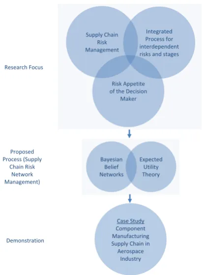
Fig. 1. Research focus and methodology.

2. Literature Review

In the following sections, we give an overview of the literature on supply chain risk management

process and interdependency modelling of supply chain risks.

2.1. Supply Chain Risk Management Process/Framework

SCRM is “the identification and management of risks for the supply chain, through a co-ordinated

approach amongst supply chain members, to reduce supply chain vulnerability as a whole” (Jüttner

et al., 2003, p. 201). Several risk management frameworks have been proposed using different

terminology; however, there is a consensus that the SCRM process involves five sequential stages:

risk identification; assessment; analysis; treatment; and monitoring (Giannakis & Papadopoulos, Demonstration

Research Focus

Supply Chain Risk Management

Integrated Process for interdependent risks and stages

Bayesian Belief Networks

Case Study Component Manufacturing Supply Chain in Aerospace

Industry Risk Appetite of the Decision

Maker

Proposed Process (Supply

Chain Risk Network Management)

Expected Utility Theory

Figure 1: Research focus and methodology.

mentation of such interdependency based frameworks. Fourth, we develop propositions to elucidate the importance of accounting for interdependence of risks and risk mitigation strategies.

Responding to the call for developing and empirically evaluating a SCRM process that not only captures interdependency between risks but also integrates all stages of the process (Colicchia & Strozzi, 2012; Ho et al., 2015), we address the following research questions in this study:

RQ1: How can we develop and operationalise a SCRM process that captures interdependencies

between risks, multiple (potentially conflicting) objectives (performance measures) and risk mitigation

strategies specific to the risk appetite of a decision maker?

RQ2: What are the merits and challenges associated with the implementation of the proposed

process?

1 2 3 4 5 6 7 8 9 10 11 12 13 14 15 16 17 18 19 20 21 22 23 24 25 26 27 28 29 30 31 32 33 34 35 36 37 38 39 40 41 42 43 44 45 46 47 48 49 50 51 52 53 54 55 56 57 58 59 60 61 62 63

2. Literature Review

In the following sections, we give an overview of the literature on supply chain risk management process and interdependency modelling of supply chain risks.

2.1. Supply Chain Risk Management Process/Framework

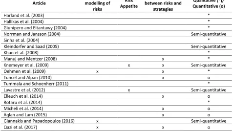
SCRM is“the identification and management of risks for the supply chain, through a co-ordinated approach amongst supply chain members, to reduce supply chain vulnerability as a whole” (J¨uttner et al., 2003, p. 201). Several risk management frameworks have been proposed using different ter-minology; however, there is a consensus that a SCRM process involves five sequential stages: risk identification; assessment; analysis; treatment; and monitoring (Giannakis & Papadopoulos, 2016). Selected articles conforming to the research focus of the paper (see Figure 1) have been classified into four categories including interdependency modelling of risks, the risk appetite of a decision maker, interdependency between risks and strategies, and research methodology as shown in Table A.1 (see Appendix A).

Ritchie & Brindley (2007) identified five components of a SCRM process: risk drivers (primary and secondary level); risk management influencers (rewards, supply chain risks, timescales, portfolio); decision maker characteristics (perceptions, risk profile, attitudes, experiences); risk management re-sponses (risk taking, avoidance, mitigation, monitoring); and performance outcomes (profit related, strategic positioning, personal). We will briefly describe the merits of some of the frameworks proposed in the literature, and delineate the main limitations of these.

A number of qualitative frameworks have been proposed to identify risks and prescribe generalised strategies to deal with important risks. These frameworks generally utilise qualitative scales to discre-tise the conventional risk matrix across the probability and impact levels. Utilising a Failure Modes and Effects Analysis (FMEA) based technique, Sinha et al. (2004) developed a process to manage risks in the aerospace industry whereas Giannakis & Papadopoulos (2016) proposed a risk management pro-cess to identify and manage sustainability related risks across the environmental, social and economic facets with its application demonstrated through empirical case studies and a survey questionnaire. Khan et al. (2008) reported the conventional risk matrix based process used in a major UK retailer that helps the company deal with design oriented supply chain risks. Bringing the perspective of a global supply chain and consolidating the concepts from logistics, supply chain management, operations management, strategy and international business management, Manuj & Mentzer (2008) proposed a procedure to help global supply chain managers identify risks and select appropriate strategies.

1 2 3 4 5 6 7 8 9 10 11 12 13 14 15 16 17 18 19 20 21 22 23 24 25 26 27 28 29 30 31 32 33 34 35 36 37 38 39 40 41 42 43 44 45 46 47 48 49 50 51 52 53 54 55 56 57 58 59 60 61 62 63

pharmaceutical supply chain case study. Similarly, Aqlan & Lam (2015) proposed a hybrid approach of bow-tie analysis and stochastic integer programming to identify critical risks and assess suitable strategies taking into account their cost and effectiveness in reducing the risk exposure. Systems thinking has also been applied to develop a comprehensive process both in its qualitative (Oehmen et al., 2009) and quantitative forms (Ghadge et al., 2013).

There are mainly three limitations of the existing frameworks including the aforementioned studies. First, the frameworks have drawn limited focus on modelling the common cause failures and assessing their propagation impact. As such common cause failures can have a far reaching impact on the efficiency of a supply network, there is a need to model and evaluate such factors (Ho et al., 2015). Second, researchers generally focus on limited stages of the risk management process whereas “there is a significant relationship between all SCRM processes, (therefore) more attention should be given

to legitimately integrated processes instead of individual or fragmented processes. ... Similarly, the

effectiveness of risk mitigation strategies requires explicit quantification of effectiveness and efficiency

of such strategies” (Ho et al., 2015, p. 5053). Third, there has been a very limited focus on the need for integrating risk appetite in the risk management process as Heckmann et al. (2015) argue that“More advanced (context-sensitive) approaches especially with respect to the risk attitude of the decision maker

and with respect to the environment of the affected supply chain are needed” (Heckmann et al., 2015, p. 130). We endeavour to fill the mentioned gaps by developing and empirically evaluating an integrated SCRNM process to establish how practitioners perceive correlations between risks specific to their risk appetite and whether they are able to evaluate the impact of risk mitigation strategies on the network of risks.

2.2. Interdependency Modelling of Supply Chain Risks

Various models have been proposed to capture interdependency between supply chain risks. In-terpretive structural modelling (ISM) is a hierarchy based technique that establishes the order and direction of complex relationships among elements of a system. It has been used to determine causal relationships between risk mitigation strategies (Faisal et al., 2006) and supply chain risks (Pfohl et al., 2011). Related to the same family of causal mapping techniques, fishbone diagram has been utilised to identify cause-effect relationships between risks (Lin & Zhou, 2011). Mapping a supply network as a web of interconnected nodes, measures from the Social Network Analysis have been adapted to identify critical supply nodes (Kim et al., 2011). The main limitation of aforementioned techniques is the inability to capture the strength of interdependency between risks.

1 2 3 4 5 6 7 8 9 10 11 12 13 14 15 16 17 18 19 20 21 22 23 24 25 26 27 28 29 30 31 32 33 34 35 36 37 38 39 40 41 42 43 44 45 46 47 48 49 50 51 52 53 54 55 56 57 58 59 60 61 62 63

ated with each risk. It has been extensively used in SCRM to identify critical risks (Nepal & Yadav, 2015; Dong & Cooper, 2016). Similarly, utilising established techniques from the field of reliability engineering, Aqlan & Lam (2015) proposed a bow-tie analysis based process to capture the interde-pendency of supply chain risks whereas Oehmen et al. (2009) and Sherwin et al. (2016) introduced FTA based frameworks to assess risks. The main problem with these techniques is their limited focus on capturing common cause failures. Although the conventional FTA does not capture common cause failures, the technique following a top-down approach is helpful in terms of brainstorming the causes of a consequence and is widely used in the literature on engineering risk management (Sherwin et al., 2016).

Mainly, supply chain risks are classified into distinct categories like process, control, demand, supply and environmental risks (Christopher & Peck, 2004). The first two risk categories relate to factors internal to an organisation, the third and fourth include factors internal to the supply chain, but external to the organisation and the fifth category relates to factors external to the supply chain. Similar to the concept of mapping causal chains in project risk management (Ackermann et al., 2014), Badurdeen et al. (2014) proposed a risk taxonomy capturing interdependency between supply chain risks that is in contrast with the established classification schemes.

In response to the call for understanding the relationships between a set of strategies for managing risks and corresponding impact on performance measures (Colicchia & Strozzi, 2012), a few models have been developed (Micheli et al., 2014; Aqlan & Lam, 2015); however, these models do not explicitly capture interdependency between risks. Another issue relates to the focus of these models on “min-imising cost or max“min-imising profit as a single objective” (Colicchia & Strozzi, 2012, p. 412) as “purely cost-and waste-considering objectives, however, evaluate supply chain’s performance in retrospect. They

miss to assess both operational effectiveness and important strategic achievements like product quality

and customer satisfaction” (Heckmann et al., 2015, p. 130). In this study, we overcome the limitation of earlier studies by not only capturing interdependencies between risks but also across the entire risk management process. We also consider optimising a set of potentially conflicting performance measures within an interdependent setting of interacting risks and strategies, and propose a new technique for prioritising risk mitigation strategies subject to a budget constraint.

2.2.1. Application of Bayesian Belief Networks in Supply Chain Risk Management

1 2 3 4 5 6 7 8 9 10 11 12 13 14 15 16 17 18 19 20 21 22 23 24 25 26 27 28 29 30 31 32 33 34 35 36 37 38 39 40 41 42 43 44 45 46 47 48 49 50 51 52 53 54 55 56 57 58 59 60 61 62 63

Article

Attributes

Lockamy and McCormack

(2009)

Dogan and Aydin

(2011)

Leerojanap rapa et al. (2013)

Badurdeen et al. (2014)

Garvey et al. (2015)

Nepal and Yadav (2015)

Hosseini and Barker

(2016)

Qazi et al. (2017)

This paper

Risk

identification x x x x x x x x x

Risk analysis/

evaluation x x x x x x x x x

Risk treatment x x

Risk appetite x

Multiple SC performance measures

x

Modelling of supply network risks

x x x x

New risk

measures x x x

Real Case Study x x x x X

Techniques BBNs BBNs BBNs BBNs BBNs FMEA and

BBNs BBNs

FMEA, BBNs, Game Theory

FTA, BBNs,

EUT, MCDA

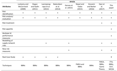
Table 1: Comparison of the Proposed Approach with Existing BBN Based SCRM Models.

framing and operationalising a comprehensive risk management process integrating suitable techniques across all stages of the process. Furthermore, the merits and challenges involved in implementing such a framework remain unexplored. A comparison of the merits of this paper with existing studies is presented in Table 1.

1 2 3 4 5 6 7 8 9 10 11 12 13 14 15 16 17 18 19 20 21 22 23 24 25 26 27 28 29 30 31 32 33 34 35 36 37 38 39 40 41 42 43 44 45 46 47 48 49 50 51 52 53 54 55 56 57 58 59 60 61 62 63

establishing the network structure that necessitates adapting BBNs to the context of SCRM whereas the literature does not provide an illustration of developing such models.

Leerojanaprapa et al. (2013) and Leerojanaprapa (2014) proposed a generic BBN modelling pro-cess to support supply chain risk analysis based on expert knowledge and conducted a case study in the medical supply chain to demonstrate its efficacy. In their effort to capture the probabilistic interdependency between supply chain risks, Garvey et al. (2015) introduced an algorithm to map risks and proposed supply chain risk measures. The main limitation of these studies is their focus on limited stages of the risk management process and ignoring the risk appetite of a decision maker. Also, modelling of risks in accordance with the process flow of a supply chain makes it infeasible to capture risks relating to substantial supply networks. However, these studies serve to illustrate the efficacy of BBNs in modelling and managing supply chain risks as BBNs can effectively measure the propa-gation impact of these risks within a network setting. Utilising BBNs, Qazi et al. (2017) introduced probabilistic supply chain risk measures to prioritise interdependent risks and strategies. Although one of the measures introduced captures an aversion to risk, the entire risk management process does not explicitly model the risk attitude (utility) of a decision maker and also, the process only helps in optimising a portfolio of strategies specific to a single performance measure (objective) rather than considering multiple (potentially conflicting) measures (objectives). We endeavour to fill these gaps through introducing and operationalising a comprehensive SCRNM process that adapts key features of established techniques from safety and reliability engineering, decision making under uncertainty and multi-criteria decision analysis to the context of SCRM.

3. Proposed SCRNM Process

1 2 3 4 5 6 7 8 9 10 11 12 13 14 15 16 17 18 19 20 21 22 23 24 25 26 27 28 29 30 31 32 33 34 35 36 37 38 39 40 41 42 43 44 45 46 47 48 49 50 51 52 53 54 55 56 57 58 59 60 61 62 63

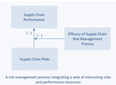
A risk management process integrating a web of interacting risks and performance measures

Supply Chain Performance

Supply Chain Risks

Efficacy of Supply Chain Risk Management

Process

the mentioned theme: first, these studies focus on few stages of the risk management process without establishing and validating a comprehensive risk management process in such projects; and secondly, interdependency modelling of risks is ignored in entirety or few studies involving interdependency do not capture common cause failures and/or optimise a single objective or a set of objectives in isolation. To fill this gap, we conduct one of the case studies in a project driven supply chain and validate the adapted process proposed by Qazi et al. (2016).

3. Proposed Process

As shown in Figure 1, the main purpose of the study is to adapt the already proposed risk management process namely ‘ProCRiM’ (Qazi et al., 2016) to the context of SCRM and validate the process. In principle, we focus on two distinct application areas: the first being a conventional supply chain that necessitates modifying ProCRiM to only focus on the interaction of supply chain risks and their influence on the supply chain performance measures (see Figure 2); the second relates to a project driven supply chain where ProCRiM is directly applicable though the risks considered are exclusively related to the supply chain (see Figure 3) whereas the focus of ProCRiM is on project related risks.

There are many studies in the literature with exclusive focus on the impact of supply chain risks on the performance measures (Zhao et al., 2013, Jüttner et al., 2003). However, we consider the impact of risk network on the performance measures whereas there is a moderating effect of the risk management process in terms of its efficacy in mitigating risks. The efficacy of risk management process in turn needs to be evaluated within a network setting. The framework shown in Figure 2 is exclusively applicable to any type of supply chain that is not involved in the NPD project.

Figure 2 Supply chain risk management framework for conventional supply chains [adapted from Jüttner et al. (2003)]

Considering the scarcity of studies on managing supply chain risks associated with NPD, Figure 3 reflects the impact of project characteristics on the supply chain risks that influence the performance measures. However, it is interesting to note that the project characteristics

( - ) _{( - )}

Figure 2: Supply chain risk management framework (adapted from J¨uttner et al. 2003).

maker also helps in identifying the key performance measures pertinent to the supply chain.

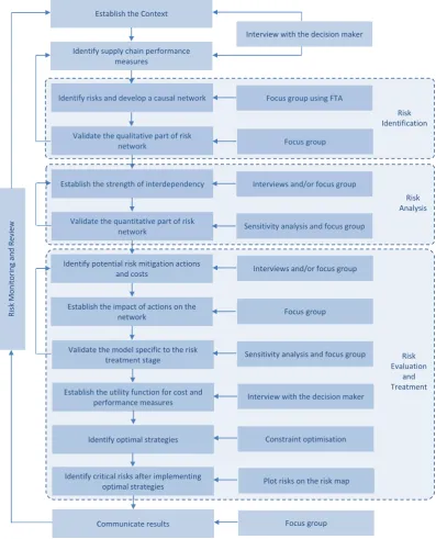
A focus group session must be conducted to identify risks and develop a causal network. We found it very useful to develop the causal network using the top-down approach where the informants were asked to link each performance measure with the corresponding risk(s) that were in turn linked back to causal factors. In a way, it mimics the technique adopted in conventional FTA (Sherwin et al., 2016); however, FTA does not capture the common-cause failures whereas we model such factors in our framework. Studies on developing the qualitative part of the BBNs and causal maps are useful in establishing the risk network (Nadkarni & Shenoy, 2004). Once the qualitative network is developed, there is a need to validate the structure and ensure whether all relevant risks have been considered. A focus group session involving all participants from the previous session and adding some new members is helpful in refining the structure and adding some missing risks. It is important to note that it is an iterative process until the final structure is validated and the participants are satisfied with the structure of the risk network.

The next stage relates to the quantitative modelling of the already validated qualitative risk network where the participants establish the strength of interdependency between the risks either through semi-structured interviews or a focus group session. Once all the conditional probability values have been elicited, a focus group session must be held to validate the model. Again studies specific to the quantitative modelling of BBNs are useful in developing and validating the model (Norrington et al., 2008). Sensitivity analysis is carried out to evaluate the impact of individual risks on each performance measure and ascertain whether the results make sense and conform to the perception of the participants. In case of any discrepancy, the quantitative model is revisited and amendments incorporated until the sensitivity results are agreed upon.

1 2 3 4 5 6 7 8 9 10 11 12 13 14 15 16 17 18 19 20 21 22 23 24 25 26 27 28 29 30 31 32 33 34 35 36 37 38 39 40 41 42 43 44 45 46 47 48 49 50 51 52 53 54 55 56 57 58 59 60 61 62 63

Establish the Context

Interview with the decision maker

Identify supply chain performance measures

Identify risks and develop a causal network Focus group using FTA

Validate the qualitative part of risk

network Focus group

Establish the strength of interdependency Interviews and/or focus group

Validate the quantitative part of risk

network Sensitivity analysis and focus group

Identify potential risk mitigation actions

and costs Interviews and/or focus group

Establish the impact of actions on the network

Establish the utility function for cost and performance measures

Identify optimal strategies

Focus group

Interview with the decision maker

Constraint optimisation

Communicate results Focus group

Validate the model specific to the risk

treatment stage Sensitivity analysis and focus group

Identify critical risks after implementing

optimal strategies Plot risks on the risk map

Risk Mo

nitori

n

g

an

d Rev

ie

w

Risk Identification

Risk Analysis

Risk Evaluation

and Treatment

1 2 3 4 5 6 7 8 9 10 11 12 13 14 15 16 17 18 19 20 21 22 23 24 25 26 27 28 29 30 31 32 33 34 35 36 37 38 39 40 41 42 43 44 45 46 47 48 49 50 51 52 53 54 55 56 57 58 59 60 61 62 63

of risk mitigation strategies. The decision maker is again consulted to determine the utility function corresponding to the performance measures and the cost of strategies. The model is subsequently run for all possible combinations of strategies subject to various budget constraints and the strategies are selected that maximise the overall expected utility of the decision maker. Finally, a focus group session is conducted to communicate the results to the participants and help the decision maker understand the impact of implementing different combinations of strategies. As risk management is a continuous process, the entire process is repeated requiring minimal changes in the model once new risks are discovered and updated.

4. Methodology

An important aim of this study is to empirically evaluate the proposed process through a case study in order to demonstrate the application of the process and establish the benefits and challenges associated with its implementation. The empirical evaluation of the process involved establishing the context of a specific organisation (case) and developing a model based on how the decision makers perceived interdependencies between risks and why certain risks and performance measures were given due importance (study). As the “case study method is an appropriate choice for investigating ‘how’ and ‘why’ questions” (Yin, 2009, p. 27), we adopted the same methodology to address the research questions.

Aero (a leading global technology provider) was selected for conducting the case study as their risk managers were keen on improving the risk management process within the company and assessing the merits and challenges of our proposed process. The initial interview protocol was piloted with Zanardi Fonderie (an Italian global manufacturing company specialising in the heat treatment of iron and its alloys) that helped in revising the questions to clarify the terms and adopting a well-structured method to develop the risk network in the case study. The main data collection method was semi-structured interviews as“the overwhelming strength of the face-to-face interview is the ‘richness’ of the communication that is possible” (Gillham, 2000, p. 62) and “the semi-structured interview is the most important form of interviewing in case study research and it can be the richest single source of data”

(Gillham, 2000, p. 63). As our research involved developing a risk network, the case study design utilised a mix of quantitative and qualitative evidence.

1 2 3 4 5 6 7 8 9 10 11 12 13 14 15 16 17 18 19 20 21 22 23 24 25 26 27 28 29 30 31 32 33 34 35 36 37 38 39 40 41 42 43 44 45 46 47 48 49 50 51 52 53 54 55 56 57 58 59 60 61 62 63

and deduced themes were shared with the interviewees for validation. Besides interviews, secondary data including publicly available corporate reports, case studies and annual performance reports were collected and analysed in order to triangulate the data collected through interviews and focus group sessions. Finally, a case study report was prepared and shared with the company to validate the authenticity of results and help the participants identify any issues.

4.1. Proposed Modelling Approach

A number of techniques including but not limited to AHP, Analytical network process, Fuzzy set theory, ISM, Network theory, FMEA and hybrid methods integrating these have been extensively used in modelling supply chain risks. The main limitation of these techniques is the inability to comprehensively capture probabilistic interdependency between risks and to propagate and update beliefs upon receiving new information. Based on the efficacy of BBNs in capturing interdependencies between risks, we consider BBN based modelling of a risk network as an effective approach. Such a modelling technique can help managers visualise supply chain risks and take effective mitigation strategies. BBNs have already been explored in the literature on risk management (Ashrafi et al., 2015; Wu et al., 2015) and SCRM (Garvey et al., 2015; Nepal & Yadav, 2015; Qazi et al., 2017) for modelling and assessing risks. However, to the best of the authors’ knowledge, BBNs have not been explored in the literature on SCRM to establish the impact of supply chain risks on multiple (potentially conflicting) objectives and to prioritise supply chain risk mitigation strategies considering the risk appetite of a decision maker. Another contribution of the proposed approach relates to the adaptation of established techniques from safety and reliability engineering, decision making under uncertainty and multi-criteria decision analysis, and integrating these together to operationalise the proposed process.

1 2 3 4 5 6 7 8 9 10 11 12 13 14 15 16 17 18 19 20 21 22 23 24 25 26 27 28 29 30 31 32 33 34 35 36 37 38 39 40 41 42 43 44 45 46 47 48 49 50 51 52 53 54 55 56 57 58 59 60 61 62 63

through the use of established interdependency based models and maintenance (and accident) data recorded whereas such data is not readily available in the case of supply chain risks as practitioners rely on risk matrix based tools and interdependency modelling is generally ignored (Leerojanaprapa, 2014). Therefore, there is a need to adapt the interdependency based tools commonly used in other areas to the context of SCRM such that the complexity associated with supply chain risks is managed effectively and the tools developed fit well with the requirements and competence of practitioners who prefer to use simple risk matrix based tools.

In order to capture the risk appetite of a decision maker, we make use of EUT. However, instead of utilising the conventional technique to elicit a decision maker’s preference over the entire combination of risks, we introduce a new approach of mapping the combination of risks to a set of performance measures making it feasible for capturing the risk appetite over a substantial risk network. This adaptation not only reduces the elicitation burden of ascertaining utility values but also helps in evaluating risks specific to global supply chains where the complex nature of interdependency between risks is not amenable to conventional SCRM techniques. Integrating BBNs with EUT provides an added benefit as besides modelling interdependency between risks, the utility for both risk appetite and trade-off across performance measures is exclusively captured whereas modelling these features in silo would undermine the integrated effect of the complex interactions involved. As such, the complexity relates to the interdependent nature of supply chain risks, non-linear interactions between risks and performance measures, utility of the decision maker with regards to the trade-off across these measures, and their risk appetite in terms of establishing the maximum level of risk exposure and the utility of risk mitigation with regards to the cost incurred in introducing strategies. Our approach deals with capturing this complexity in a unique manner and integrates all these features in a holistic framework. In the following sections, we provide a brief overview of the BBNs and EUT as these have been used to develop the proposed modelling approach.

4.1.1. Bayesian Belief Networks

BBN is a graphical framework for modelling uncertainty. BBNs have their background in statis-tics and artificial intelligence and were first introduced in the 1980s for dealing with uncertainty in knowledge-based systems (Sigurdsson et al., 2001). They have been successfully used in addressing problems related to a number of diverse specialties including reliability modelling, medical diagnosis, geographical information systems, and aviation safety management among others. For understand-ing the mechanics and modellunderstand-ing of BBNs, interested readers may consult Sigurdsson et al. (2001); Nadkarni & Shenoy (2004); Jensen & Nielsen (2007). A BBN consists of the following elements:

1 2 3 4 5 6 7 8 9 10 11 12 13 14 15 16 17 18 19 20 21 22 23 24 25 26 27 28 29 30 31 32 33 34 35 36 37 38 39 40 41 42 43 44 45 46 47 48 49 50 51 52 53 54 55 56 57 58 59 60 61 62 63

no directed pathX1→...→Xnso thatX1 =Xn, furthermore, the directed edges represent sta-tistical relations if the BBN is constructed from the data whereas they represent causal relations if they have been gathered from experts’ opinion,

• A conditional probability tableP(X|Y1, ...Yn) attached to each variableXwith parentsY1, ..., Yn.

Chain Rule for Bayesian Belief Networks. Let a Bayesian Network be specified over X =X1, ..., Xn.

The structure of a BBN implies that the value of a particular node is conditional only on the values of its parent nodes. Therefore, the unique joint probability distribution P(X) representing the product of all conditional probability tables is given as follows:

P(X) =

n

Y

i=1

P(Xi|pa(Xi)) (1)

where pa(Xi) are the parents of Xi.

Merits and Challenges. BBNs present a useful technique for capturing interdependency between supply chain risks (Badurdeen et al., 2014). Another advantage of using BBNs for modelling supply chain risks is their ability of back propagation that helps in determining the probability of an event that may not be observed directly. They provide a clear graphical structure that most people find intuitive to understand. Besides, it becomes possible to conduct flexible inference based on partial observations, which allows for reasoning. Another important feature of using BBNs is to conduct what-if scenarios. There are certain problems associated with the use of BBNs: along with the increase in number of nodes representing uncertain variables, a considerable amount of data is required in populating the network with (conditional) probability values; similarly, there are also computational challenges associated with the increase in number of nodes.

4.1.2. Expected Utility and Decision Making under Uncertainty

Within the context of decision making under uncertainty, risk can be related to a utility function that reflects the preferences of a decision maker with regard to various possible consequences of a decision. Expected utility theory posits that a decision-maker’s preferences over an outcome xcan be represented by a utility function u(x), and if there arei= 1, . . . , n possible states of the world each of which occurs with probabilitypi and in which the outcome is xi then the decision-maker cares about

their expected utility Pn

1 2 3 4 5 6 7 8 9 10 11 12 13 14 15 16 17 18 19 20 21 22 23 24 25 26 27 28 29 30 31 32 33 34 35 36 37 38 39 40 41 42 43 44 45 46 47 48 49 50 51 52 53 54 55 56 57 58 59 60 61 62 63

4.1.3. Proposed Approach

Although EUT provides a standardised normative framework to make decisions under uncertainty, it is not so much used in practice mainly because of the difficulty associated with assigning utility values to all possible outcomes (Aven & Kristensen, 2005). If a network consists of N risks each of which has binary outcomes then there are 2N utility values that must be elicited, which is potentially a very large number. To circumvent this difficulty, we introduce a new approach to evaluating a network of interconnected risks.

Let a risk network be combined of j = 1, . . . , N interdependent binary risks denoted Rj that can take the value ‘true’ or ‘false’. Rather than assessing the state of each risk, it will be assumed that the combination of these risks can be summarised in M < N binary performance measures denoted ml,

l= 1, . . . , M, that can take the value ‘good’ or ‘bad’. The probability that each risk is realised in the network combines to determine the probability of each performance measure being ‘good’ or ‘bad’.

A state of the network is a particular realisation of performance measures, each of which can be either ‘good’ or ‘bad’. We denote a typical state si ∈ {good, bad}M_{; there are 2}M _{possible states in the}

set of states that we denote byI. Decision makers are assumed to evaluate a realisation of the network in a particular state by the combination of performance measures that are realised in that state. As such, we define the decision-maker’s utility function as

u:{good, bad}M →[0,1] (2)

where utility evaluations are scaled to take a value on the unit interval. The probability that state i

occurs is the joint probability that each of the performance measures takes its value specified by the state, that we denote pi. Decision makers are then assumed to evaluate the expected utility of the

network:

EU =X

i∈I

piu(si). (3)

As the state of risks influences performance measures, we introduce the notion of risk propagation measure (RP M) to capture the relative impact of each risk on the set of performance measures modelled within a risk network. RP Mj is the probability weighted expected utility of the network if risk j is

realised.

RP Mj =p(Rj =true)EU|Rj =true. (4)

1 2 3 4 5 6 7 8 9 10 11 12 13 14 15 16 17 18 19 20 21 22 23 24 25 26 27 28 29 30 31 32 33 34 35 36 37 38 39 40 41 42 43 44 45 46 47 48 49 50 51 52 53 54 55 56 57 58 59 60 61 62 63

form a mitigation strategy and we denote a typical risk mitigation strategy by σk. We letσ0 denote the (costless) strategy ‘do nothing’ so the network is in its original configuration; σ₂A₋₁ means do everything. There are 2A combinations of risk mitigation actions (including doing nothing) in the set of mitigation strategies that we denote K. By undertaking a risk mitigation strategy the probability with which each state of the network (in terms of performance measures) is realised is influenced, and therefore we write these probabilities as a function of the risk mitigation strategy adopted,pi(σk). Risk

mitigation is a costly exercise; we write Ck as the cost of undertaking the strategyσk. To evaluate a realisation of the network after undertaking a mitigation strategy, we should write a decision-maker’s utility as a function of both si, the state of the performance measures andCk, the cost of mitigation, so the expected utility resulting from undertaking risk mitigation strategyk would be

X

i∈I

pi(σk)U(si, Ck).

However, operationally this specification would require that we elicit utility values over each state of the network in every possible cost realisation, which is often not feasible. To circumvent this problem, we assume that utility is separable in the evaluation of the state of the network and the cost of mitigation (Wilson & Quigley, 2016). To scale the evaluation of the cost of mitigation strategies we define a utility value for the cost v(Ck) that yields a utility of 1 if there is no cost and then reduces

to a minimum value of zero as the cost of mitigation increases. Further, we consider a ‘weighted net evaluation’ (WNE) of a mitigation strategy, which is defined as

W N E(σk) = (1−α)EU(σk) +αv(Ck) (5)

where

EU(σk) =X

i∈I

pi(σk)u(si). (6)

1 2 3 4 5 6 7 8 9 10 11 12 13 14 15 16 17 18 19 20 21 22 23 24 25 26 27 28 29 30 31 32 33 34 35 36 37 38 39 40 41 42 43 44 45 46 47 48 49 50 51 52 53 54 55 56 57 58 59 60 61 62 63

Problem of Selecting Optimal Risk Mitigation Strategies. Having defined the way in which decision makers assess the outcome of undertaking a mitigation strategy, we now define the objective function of a decision maker, which is to choose the mitigation strategy that maximises the WNE of risk mitigation, subject to the constraint that the cost of mitigation must not exceed a threshold, ¯C:

max

σk∈K

W N E(σk) s.t. Ck≤C.¯

5. Application of the Proposed Process

5.1. Description of the Case Study

Founded in the early 20th Century, Aero is a leading global supplier of products, solutions and services within rolling bearings, seals, mechatronics, services and lubrication systems. Having 120 manufacturing units established in 29 countries and a distribution network across 130 countries, Aero serves a diversified mix of industries, including cars and light trucks, marine, aerospace, renewable energy, railway, metal, machine tool, medical and food and beverage.

The respondents were selected on the basis of their expertise in risk management in general and SCRM/project risk management in particular. A total of seven semi-structured interviews were con-ducted with details of the experts given in Table A.2. Each interview lasted for 90 minutes on average (with the minimum and maximum time of 70 and 120 minutes, respectively). A total of three focus group sessions were also held involving the development and validation of the model and communication of the results with each session lasting for 2 hours on average.

5.2. Model Development and Results

Five performance objectives namely quality, timeliness, market share, profit and sustainability were identified during the interviews. These objectives are interrelated as market share influences the profit margin and also, quality, timeliness and profit are potentially conflicting objectives. Instead of following a bottom-up approach as adopted in the Event Tree analysis, we developed the network using the FTA that utilises a top-down approach. The network was developed involving two members from the risk management group. They were asked to focus on a one-year time horizon and assess the probability of risks within that timeframe. Furthermore, the main focus was on identifying only main risks that would ultimately influence the performance objectives of the company. This exercise of brainstorming and linking risks to the performance measures identified (as used in the FTA) was guided by the principles of modelling a BBN (Nadkarni & Shenoy, 2004).

1 2 3 4 5 6 7 8 9 10 11 12 13 14 15 16 17 18 19 20 21 22 23 24 25 26 27 28 29 30 31 32 33 34 35 36 37 38 39 40 41 42 43 44 45 46 47 48 49 50 51 52 53 54 55 56 57 58 59 60 61 62 63

risks presented in Table A.3. One main feature of the developed structure is capturing interdependency between risks ranging across different categories namely supply, demand, process and control risks (Christopher et al., 2011) and therefore, instead of conceptualising risks into distinct categories, we focus on intra- and inter- dependency across all such categories in the form of a risk network as shown in Figure 5. Control risks represent the problems associated with the management policies and these can be considered as the common causes affecting the entire network of risks as shown in Figure 4. For example, poor management policies might adversely affect the motivation of employees which in turn would influence the production rate and even the quality might be compromised triggering customer dissatisfaction.

Following the qualitative validation of the risk network, another focus group session was held to quantify the model. Two of the participants were engineers and well conversant with the fundamentals of probability theory and therefore, it was not difficult to elicit conditional probability values. However, not all participants were comfortable with providing the probability values. Therefore, a qualitative scale was introduced to elicit probability and utility values as shown in Figure A.1 and Figure A.2, respectively.

The quantitative part was validated through conducting the sensitivity analysis during which some conditional probability values had to be revised as the participants were not satisfied with some of the sensitivity results. The updated probabilities of the quality (low), timeliness (delayed), market share (low), profit (low) and sustainability (low) were calculated as 0.35, 0.08, 0.68, 0.60 and 0.33, respectively. The (red) shade of a node represents its relative importance for the utility node in terms of the propagation impact whereas the thickness of an arc reflects the strength of interdependency (influence) between the interconnected nodes. The participants agreed with the optimistic results for quality, timeliness and sustainability and somehow justified their concern with regard to the higher probabilities associated with market share and profit. The results also conformed to their perception about the efficacy of already implemented strategies.

The decision maker was interviewed to determine the ‘utility’ associated with different values of the objectives as shown in Table A.4 and potential mitigation strategies were identified during another focus group session with associated costs shown in Table A.5. The strategies were finally mapped on the risk network as shown in Figure A.3 and the impact of each strategy was established through eliciting the relevant conditional probability values. The rectangular shaped nodes (except the objectives appearing at the top) represent all possible strategies. Once all the potential strategies were implemented, the updated probabilities of the quality (low), timeliness (delayed), market share (low), profit (low) and sustainability (low) were calculated as 0.23, 0.05, 0.37, 0.33 and 0.24, respectively. The efficacy of strategies elicited was validated through conducting sensitivity analysis.

1 2 3 4 5 6 7 8 9 10 11 12 13 14 15 16 17 18 19 20 21 22 23 24 25 26 27 28 29 30 31 32 33 34 35 36 37 38 39 40 41 42 43 44 45 46 47 48 49 50 51 52 53 54 55 56 57 58 59 60 61 62 63 Lo w 35 % H ig h 65 % Q ua lit y D el ay ed 8% T im el y 92 % T im el in es s Lo w 68 % H ig h 32 % M ar ke t S ha re Lo w 33 % H ig h 67 % S us ta in ab ili ty Y es 22 % N o 78 % S up pl ie rs Q ua lit y Pr .. . Y es 24 % N o 76 % A er o In te rn al Q ua lit .. . Y es 10 % N o 90 % La ck o f P ro ce du re s Y es 10 % N o 90 % La ck o f C on tr ol Y es 23 % N o 77 % H um an r el at ed is su es Y es 39 % N o 61 % La ck o f P ro ce du re s Y es 5% N o 95 % La ck o f C on tr ol Y es 14 % N o 86 % H um an r el at ed is su es Y es 9% N o 91 % S up pl ie rs P ro bl em s Y es 17 % N o 83 % A er o M an uf ac tu ri ng .. . Y es 12 % N o 88 % S up pl ie r di sr up tio n Y es 10 % N o 90 % Lo gi st ic s P ro bl em B ad 39 % G oo d 61 % R M C ul tu re B ad 61 % G oo d 39 % B C M C ul tu re Lo w 60 % H ig h 40 % P ro fit H ig h 90 % Lo w 10 % A er o P ri ce v s co m p. .. Lo w 46 % H ig h 54 % A er o Q ua lit y vs c o. .. Y es 10 % N o 90 % S up pl ie rs p ro bl em . .. Y es 36 % N o 64 % A er o pr ob le m w ith . .. Y es 12 % N o 88 % P ol lu tio n Y es 7% N o 93 % La bo r re la te d di se as e Y es 4% N o 96 % F at al a cc id en t Y es 31 % N o 69 % B re ak o f co de o f co .. . B ad 25 % G oo d 75 % C or po ra te G ov er na .. . U til ity Y es 14 % N o 86 % S up pl ie rs M an uf ac t.. . Y es 8% N o 92 % A er o P ro bl em s Y es 12 % N o 88 % A er o di sr up tio n Y es 10 % N o 90 % U ne xp ec te d ev en ts Y es 5% N o 95 % IC T S ys te m d is ru pt io n Y es 5% N o 95 % IC T S ys te m d is ru pt io n Lo w 20 % H ig h 80 % In ve st m en t i n lo ss p .. . Y es 5% N o 95 % S tr ik es Y es 5% N o 95 % U ne xp ec te d ev en ts Y es 50 % N o 50 % C us to m er p re ss ur e .. . Y es 20 % N o 80 % C ha ng e in s pe ci fic a. .. Y es 10 % N o 90 % R eg ul at or y ch an ge s N ot _e ff ec ti .. .2 0% E ff ec tiv e 80 % C om m un ic at io n P la n Y es 10 % N o 90 % U ne xp ec te d ev en ts Y es 1% N o 99 % F in na ci al is su es Y es 10 % N o 90 % F in an ci al is su es Y es 29 % N o 71 % A er o E H S R is ks Y es 10 % N o 90 % S tr ik es Y es 10 % N o 90 % H um an e rr or Y es 5% N o 95 % S tr ik es Y es 5% N o 95 % H um an e rr or Y es 40 % N o 60 % In te rn al a nd e xt er na .. .

1 2 3 4 5 6 7 8 9 10 11 12 13 14 15 16 17 18 19 20 21 22 23 24 25 26 27 28 29 30 31 32 33 34 35 36 37 38 39 40 41 42 43 44 45 46 47 48 49 50 51 52 53 54 55 56 57 58 59 60 61 62 63

Environmental Risk

Figure 6 The relationship between supply chain risks [adapted from Christopher et al. (2011)]

The decision maker was interviewed to determine the utility function with respect to the objectives as shown in Table III and potential mitigation strategies were identified during another focus group session with associated costs shown in Table IV. The strategies were finally mapped on the risk network as shown in Figure 7 and the impact of each strategy was established through eliciting the relevant conditional probability values. The rectangular shaped nodes (except the objectives appearing at the top) represent all possible strategies. Once all the potential strategies were implemented, the updated probabilities of the quality (low), timeliness (delayed), market share (low), profit (low) and sustainability (low) were calculated as 0.23, 0.05, 0.37, 0.33 and 0.24, respectively. The efficacy of strategies elicited was validated through conducting sensitivity analysis.

INSERT TABLE III ABOUT HERE

INSERT TABLE IV ABOUT HERE

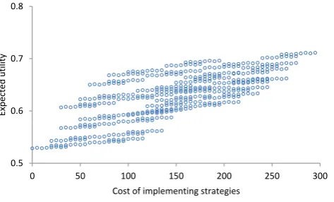
We simulated the model for each possible combination of strategies (29 _{iterations) and} evaluated the expected utility value for each instance. Subsequently, we grouped different strategies subject to a budget constraint and plotted the expected utility graph as shown in Figure 8. The variation in the expected utility value is non-linear and it is not always optimal to implement more strategies (195-235 units of cost). We also mapped the overall expected utility (net of utility and cost) corresponding to different weights assigned to the expected utility and cost as shown in Figure 9. This graph proved as a validity check as with the increase (decrease) in the preference for the expected utility (cost), the optimal solution moves away from the current investment level. Next, we determined the optimal investment level with respect to the budget constraint as shown in Figure 10. A decision maker assigning equal importance to the improvement in expected utility value and the mitigation cost must never invest in strategies costing more than 30 units. Similarly if the decision maker attributes 90% of the importance to the improvement in expected utility, the investment level should be increased to 165 units.

Supply Risk Process Risk Demand _Risk

Control Risk

Figure 5: The relationship between supply chain risks (adapted from Christopher et al. 2011).Figure 8 Variation of expected utility (across key performance measures) with mitigation

cost

Figure 9 Variation of overall expected utility (relative weight of holistic improvement in performance measures, relative weight of cost of strategies) with mitigation cost

For the sake of risk prioritisation, we mapped the updated probability of each risk with associated conditional impact on the expected utility as shown in Figure 11. The two randomly selected curves segregate the entire map into high, medium and low risk zones. Here we do not specifically focus on the criteria to establish the boundaries of these curves. R20, R26 and R11 appear to be the most critical risks. In order to gain an insight into the efficacy of implementing potential mitigation strategies, the configuration of risks is shown in Figure 12. With the same segregation of risk zones, there is no risk in the high risk zone whereas only R26 is located in the medium risk zone. Therefore, the implementation of all potential strategies helps in substantially improving the overall state of all risks.

0.5 0.6 0.7 0.8

0 50 100 150 200 250 300

Expected

utili

ty

Cost of implementing strategies

0.5 0.6 0.7 0.8

0 50 100 150 200 250 300

Cost of implementing strategies

Expected Utility Overall Expected Utility (0.9 : 0.1) Overall Expected Utility (0.7 : 0.3) Overall Expected Utility (0.5 : 0.5)

Figure 6: Variation of expected utility (specific to performance measures) with mitigation cost.

utility value evaluated for each instance. Figure 6 plots the cost and expected utility combinations for each of the strategies. If a decision maker was targetting a particular cost of implementation they should choose the strategy that gives the highest expected utility for that cost. Note that increasing the cost of mitigation does not always improve utility, as can be seen in the range 195−235 units of cost.

The maximum weighted net evaluation of risk mitigation was mapped subject to different weights assigned to the expected utility and cost of strategies as shown in Figure 7. This graph provides as a validity check as the cost of the optimal solution is decreasing as the weight attached to cost increases (higher α). Next, the optimal investment level (one maximising the W N E of risk mitigation) with respect to the budget constraint was determined as shown in Figure 8. A decision maker assigning equal importance to the improvement in expected utility value and the mitigation cost must never invest in strategies costing more than 30 units. Similarly if the decision maker attributes 90% of the importance to the improvement in expected utility, the investment level should be increased to 165 units.

1 2 3 4 5 6 7 8 9 10 11 12 13 14 15 16 17 18 19 20 21 22 23 24 25 26 27 28 29 30 31 32 33 34 35 36 37 38 39 40 41 42 43 44 45 46 47 48 49 50 51 52 53 54 55 56 57 58 59 60 61 62 63

.

0.5 0.6 0.7 0.8

0 50 100 150 200 250 300

Cost of implementing strategies

WNE (α=0) WNE (α=0.1) WNE (α=0.3) WNE (α=0.5)

0 50 100 150 200 250 300

0 50 100 150 200 250 300

Op

tim

al

Inves

tme

nt

Budget Constraint

WNE (α=0.5) WNE (α=0.3) WNE (α=0.1) WNE (α=0)

Figure 7: Variation of maximum weighted net evaluation (W N E) of risk mitigation with different importance weights

for cost (α) and mitigation cost.

.

0.5 0.6 0.7 0.8

0 50 100 150 200 250 300

Cost of implementing strategies

WNE (α=0) WNE (α=0.1) WNE (α=0.3) WNE (α=0.5)

0 50 100 150 200 250 300

0 50 100 150 200 250 300

Op

tim

al

Inves

tme

nt

Budget Constraint

WNE (α=0.5) WNE (α=0.3) WNE (α=0.1) WNE (α=0)

1 2 3 4 5 6 7 8 9 10 11 12 13 14 15 16 17 18 19 20 21 22 23 24 25 26 27 28 29 30 31 32 33 34 35 36 37 38 39 40 41 42 43 44 45 46 47 48 49 50 51 52 53 54 55 56 57 58 59 60 61 62 63

Figure 10 Optimal investment subject to different preferences (holistic improvement in performance measures, cost of strategies) and budget constraint

Figure 11 Risk matrix representing current state of risks (no potential strategies implemented)

5.2. Results: Case Study II (NSN)

We followed the similar approach adopted in the first case study. However, we could not focus on the risk treatment stage because of the time constraint. Nonetheless, we were able to validate the adapted version of ProCRiM and discuss the merits and challenges associated with implementing the proposed process. The main informant was asked to choose a particular project and identify the key performance objectives associated with the project. Cost, time, volume of activities and fitness for purpose were the main objectives identified. Following the similar approach of FTA and involving two other participants, supply chain risks were connected across the objectives and the risk network was developed as shown in Figure 13 with details of risks presented in Table V. A list of selected project complexity attributes (Qazi et al., 2016) was shared with the informant and five attributes (shown as

0 50 100 150 200 250 300

0 50 100 150 200 250 300

Op tim al Inves tme nt Budget Constraint

Overall Expected Utility (0.5 : 0.5) Overall Expected Utility (0.7 : 0.3) Overall Expected Utility (0.9 : 0.1) Expected Utility

R1 R2 R3 R4

R5

R6 R7 R8 R9 R10 R11 R12 R13 R14 R15 R16 R17 R18

R19 R20

R21 R22 R23 _R24 R26 R27 R28 0 15 30 45

0 0.2 0.4 0.6 0.8 1

Pe rcentag e dec reas e in expected utili ty Probability (Ri=True)

Figure 9: Risk matrix representing current state of risks (with no potential strategies implemented).

rectangular nodes at the bottom of Figure 13) were finally selected to have significant impact on the risk network modelled.

Figure 12 Risk matrix representing state of risks after implementation of all potential strategies

INSERT TABLE V ABOUT HERE

A focus group session was held to validate the qualitative part of the network. The presented network reflects the final version of the network that was ultimately accepted following discussion with the participants. The quantitative part of the model was developed with the help of key informant. Unlike the participants involved in the first case study, the key informant was not comfortable with providing the probability values. Therefore, a qualitative scale was introduced to elicit the probability values and utility values as shown in Figure 14 and Figure 15, respectively. The utility function elicited is presented in Table VI. As there were five project attributes considered in the model, a total of 32 different projects could be analysed. The variation of the expected utility with the project attributes is shown in Figure 16. The 1st point represents the most complex project whereas the 32nd _{point reflects the least complex project in terms of the complexity} attributes selected.

INSERT TABLE VI ABOUT HERE

We mapped all the risks on the risk matrix with associated probability value and the impact on expected utility in case of their realisation as shown in Figure 17. The graph reflects the risk configuration corresponding to the most complex project. R13, R1, R10, R5 and R3 are the most critical risks to be mitigated. If the least complex project is modelled, all the risks move to the low risk zone as shown in Figure 18. The partitioning of the risk matrix is dependent on the risk appetite of the decision maker and a standardised process can be adopted to establish the boundaries of these zones (Ruan et al., 2015).

R1 R2 R3 R4 R5 R6 R8 R9 R10

R11 R12 R13 R14 R15 R16 R17 R18 R19 R20 R21

R22 R23 _R24 R26 R27 R28 0 15 30 45

0 0.2 0.4 0.6 0.8 1

Pe rcentag e dec reas e in expected utili ty Probability (Ri=True)

Figure 10: Risk matrix representing state of risks after implementation of the strategy “do everything” (all actions).

et al. (2015), this space can be partitioned into high, medium and low risk zones by using appropriate indifference curves. Implementing a risk mitigation strategy changes the location of risks as illustrated in Figure 10, and visualising the effect of a risk strategy on the location of those risks - in particular in relation to the critical thresholds - can assist decision-makers in reaching an optimal conclusion if such thresholds exist in the decision-maker’s value system that are not captured by a simple expected utility measure.

6. Discussion and Implications

As the main aim of our research was to address two related questions, we discuss hereafter the implications of the research findings in order to explicitly address each question.

6.1. A SCRM Process Integrating Interdependent Factors and the Risk Appetite

In this section, we present a brief comparison of the proposed approach with the interdependency based approaches applied in other research areas and discuss the theoretical and managerial implica-tions of the research.

RQ1: How can we develop and operationalise a SCRM process that captures interdependencies

between risks, multiple (potentially conflicting) objectives (performance measures) and risk mitigation

1 2 3 4 5 6 7 8 9 10 11 12 13 14 15 16 17 18 19 20 21 22 23 24 25 26 27 28 29 30 31 32 33 34 35 36 37 38 39 40 41 42 43 44 45 46 47 48 49 50 51 52 53 54 55 56 57 58 59 60 61 62 63

6.1.1. Comparison of the Proposed Approach with Interdependency Based Approaches in other

Appli-cation Areas

With respect to interdependency modelling, there are a number of approaches (similar to the ones discussed in Section 2.2) applied to other application areas including but not limited to project risk management (Qazi et al., 2016; Zhang, 2016), enterprise resource planning (Aloini et al., 2012a,b) and reliability of engineering systems (Ashrafi et al., 2015). Using the unique features of BBNs and EUT, the proposed approach not only captures probabilistic interdependency between risks but also integrates the risk appetite of a decision maker within the risk management process. We are not aware of any such risk management process especially in the literature on SCRM and project risk management that utilises the concept similar to W N E or introduces the ‘probability-conditional expected utility’ matrix for prioritising strategies and risks, respectively specific to the risk appetite of a decision maker. Network theory and ISM based tools are useful in assessing the driving and dependency influence of risks (Aloini et al., 2012a,b) whereas the proposed framework integrates these key features with the ability to model strength of interdependency between risks. The risk network provides an effective visual tool to help the decision maker prioritise risks on the basis of relative probability and propaga-tion impact values thereby considering a holistic view of multiple factors including the posipropaga-tion of a risk within the network, its influence on the key performance measures identified, and its probability of occurrence. The operationalisation scheme introduced in the paper provides an opportunity for researchers from diversified fields including but not limited to safety and reliability engineering, deci-sion making under uncertainty, data analytics, and multi-criteria decideci-sion analysis to explore similar combinations of suitable techniques that could be adapted to the context of SCRM and easily adopted by practitioners.

6.1.2. Theoretical Implications

1 2 3 4 5 6 7 8 9 10 11 12 13 14 15 16 17 18 19 20 21 22 23 24 25 26 27 28 29 30 31 32 33 34 35 36 37 38 39 40 41 42 43 44 45 46 47 48 49 50 51 52 53 54 55 56 57 58 59 60 61 62 63

Bayesian Belief Networks Expected Utility Theory

Safety and Reliability Engineering Multi-Criteria Decision Analysis

Risk Identification

Risk Analysis and Evaluation

Risk Treatment

𝐸𝑈

Context specification

Optimisation

𝑅𝑃𝑀

Critical risks Risk

Re-assessment

𝑇𝑖𝑚𝑒: 𝑇 = 𝑡0 Fault Tree

Analysis

𝑇𝑖𝑚𝑒: 𝑇 > 𝑡0 Risk

Monitoring

𝑊𝑁𝐸

Risk Appetite

Swing Weights

Risk and Performance

Network

Modified Risk Matrix

Optimal strategies

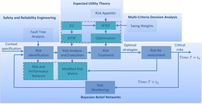
Figure 11: A block diagram representing the contribution of the proposed approach to the established risk management

process (SA, 2009).

Risk Identification. Instead of following the conventional risk classification schemes the process intro-duces development of a risk and performance network where performance measures (objectives) are identified first followed by linking risks to these measures. Adopting such a technique (similar to the FTA) helps in not only modelling material risks but also common cause failures. The participants involved in developing the risk network were able to identify around 65 connections within the net-work. Furthermore, few risks located at the bottom of the network (business continuity management culture, risk management culture) were evaluated as critical risks having major influence on a number of risks. The selection of risks material to the performance measures identified is corroborated by Figure 9 where all risks possess higher values of conditional expected utility values representing the greater strength of interdependency within the risk network.

Risk Analysis. Risk matrix based tools and interdependency based models proposed in the literature generally focus on a single performance measure (monetary loss resulting from a risk realised) (Garvey et al., 2015; Qazi et al., 2017) whereas it is important to consider all material performance measures including but not limited to quality, time, profit, competitive advantage, sustainability, cost and rep-utation. Instead of focussing on the monetary value of a loss resulting from a risk, the proposed process utilises the concept of conditional expected utility and each risk is evaluated with respect to its probability and influence on the overall expected utility across the risk network in terms of the risk propagation measure (see Equation 4). Instead of mapping each risk onto a probability-impact matrix (Khan et al., 2008; Duijm, 2015), the process introduces the ‘probability-conditional expected utility’ matrix thereby capturing the impact of each risk on all performance measures identified.