ROBUST JOINT SPARSITY MODEL FOR HYPERSPECTRAL IMAGE CLASSIFICATION
Shaoguang Huang
1, Hongyan Zhang
2, Wenzhi Liao
1and Aleksandra Piˇzurica
11
Department of Telecommunications and Information Processing, Ghent University, Belgium
2The State Key Lab. of Inform. Engineering in Surveying, Mapping, and Remote Sensing,
Wuhan University, China
ABSTRACT
Sparsity-based classification methods have been widely used in hyperspectral image (HSI) classification. These methods typically assumed Gaussian noise, neglecting the fact that HSIs are often corrupted by different types of noise in prac-tice. In this paper, we develop a robust super-pixel level joint sparse representation classification model (RSJSRC) to address the mixed noise problem in sparsity-based HSI clas-sification. Our method takes into account both Gaussian and sparse noise. Experimental results on simulated and real data demonstrate the efficiency of the proposed method and clear benefits from the introduced mixed-noise model.
Index Terms— Robust classification, hyperspectral im-age, super-pixel segmentation, sparse representation
1. INTRODUCTION
Hyperspectral images (HSIs) can provide detailed spectral information about the image objects in hundreds of narrow bands, allowing this way differentation between materials that are often visually indistinguishable. Numerous applica-tion areas include agriculture [1], defense and security [2] and environmental monitoring [3].
Classification of HSIs gains currently lots of attention in remote sensing community. The objective of supervised hyperspectral classification is to group pixels into different classes with the classifiers trained by the given training sam-ples. A large number of HSI classification methods have been proposed, based on artificial neural networks [4], multino-mial logistic regression [5], [6] and support vector machines (SVM) [7], just to name a few. With the target of exploiting spatial information in the classification task, spatial-spectral classification approaches have been developed, including SVM with composite kernels [8], methods based on math-matical morphology [9–12] and image segmentation [13].
In recent years, sparse representation classification (SRC) emerged as another effective classification approach for HSI
This work was supported by the FWO project: G.OA26.17N Dictionary Learning and Distributed Inference for the Processing of Large-scale Hetero-geneous Image Data (DOLPHIN). Wenzhi Liao is a postdoctoral researcher of the Fund for Scientific Research in Flanders (FWO).
[14–18]. It assumes that each test sample can be sparsely rep-resented as a linear combination of atoms from a dictionary, which is constructed or learned from training samples [14]. Chenet al. [14] first applied the joint sparse representation classification (JSRC) in HSI classification by incorporating spatial information. The model was based on the observation that the pixels in a patch share similar spectral characteristics and can be represented by a common set of atoms but with different sparse coefficients. Zhang et al [15] proposed a nonlocal weighted joint sparse representation (NLW-JSRC) to further improve the classification accuracy. They enforced a weigh matrix on the pixels of a patch in order to discard the invalid pixels whose class was different from that of the central pixel. In addition, other improved JSRC models [16, 19, 20] also have been proposed for the HSI classification and achieved good results.
However, previous sparsity-based methods for HSI clas-sification only take into account Gaussian noise. In real applications, HSIs are inevitably corrupted by different kinds of noise, including Gaussian noise, impulse noise, dead lines and strips [21]. Here,sparse noiseis defined as the noise of arbitrary magnitude that only affects certain bands or pixels. It may arise due to the defective pixels and poor imaging conditions such as water vapor and atmospheric effect [22]. While this effect hinders the classification performance, we are not aware of any classification method that takes it ex-plicitly into account. Therefore, it is desirable to develop a classification method which accounts for these degradations and validate its performance on real data.
val-idate it on simulated and real data. The results demonstrate improved performance in comparison to related recent meth-ods and a clear benefit resulting from the introduced noise model.
The rest of this paper is organized as follows. Section 2 introduces the classical sparsity-based models in HSI classifi-cation. Section 3 describes our proposed model and optimiza-tion algorithm. Secoptimiza-tion 4 presents experimental results with simulated and real data and Section 5 concludes the paper.
2. SPARSITY-BASED MODELS IN HSI CLASSIFICATION
2.1. Sparse representation classification
Letx ∈ RB be a test sample andD = [D1,D2, ...,DC] ∈ RB×da structured dictionary constructed from training sam-ples, where B is the number of bands in the HSI; dis the number of training samples;Cis the number of classes, and Di(i=1,2,...,C) is the sub-dictionary in which each column is a training sample ofi-th class. The goal of sparse representa-tion is to represent each test sample as
x=Dα+n, (1)
wheren ∈ RB is Gaussian noise and α ∈ Rd are sparse coefficients, satisfying
ˆ
α= arg min
α
kx−Dαk2
2 s.t. kαk0≤K. (2)
kαk0denotes the number of non-zero elements inαandK
is the sparsity level, i.e. the largest number of atoms in dictio-naryDneeded to represent any input samplex. Problem (2) is typically solved with a greedy algorithm, such as Orthogo-nal Matching Pursuit (OMP) [23].
The class of the test sample is identified by calculating the class-specific residualsri[24]:
class(x) = arg min
i=1,2,...,C
ri(x)
= arg min
i=1,2,...,C
kx−Diαik2, (3)
whereαiare the sparse coefficients associated with classi.
2.2. Joint sparse representation classification
An effective method to exploit the spatial information of the HSI is using joint sparse representation of neighbouring pix-els. The assumption is that the pixels in a small patch often belong to the same class and could share the same sparsity pattern, which means that all the neighbouring pixels can be represented by the same set of atoms but with different sets of coefficients [14]. In JSRC model, a square window is used to find the spatial neighbourhood for the central pixel and all the neighbouring pixels are stacked as the input matrixXpa=
[x1,x2, ...,xT]∈RB×T, wherexiare the spectral signatures of pixels in one patch of size√T×√T.Xpais approximated by dictionaryDand row-sparse matrixApa ∈
Rd×T as fol-lows:
Xpa=DApa+N. (4)
The sparse matrix Apa can be obtained by solving the following problem [25]:
ˆ
Apa= arg min
Apa
kXpa−DApak2
F
s.t.kApakrow,0≤K0, (5)
wherekApakrow,0 denotes the number of non-zero rows of
Apa andK0 is the row-sparsity level. In a similar way to SRC, the central test pixel of the patch is labeled by calculat-ing the class-specific reconstruction errors:
class(xcentral) = arg min i=1,2,...,C
kXpa−DiApai kF, (6)
whereApai is the portion of sparse matrix Apa associated with classi.
3. PROPOSED METHOD
In practice, HSI is often corrupted by multiple noises. Next to the Gaussian noise in (4), degradation like impulse noise, dead lines and strips are typically also present. We call these degradations sparse noise because they only corrupt relatively few pixels in HSI. We extend the model ofXpain (4) as:
Xpa=DApa+Spa+N, (7) whereSpa ∈ RB×T is the sparse noise ofXpa. In order to better exploit the spatial information of HSI, we perform the HSI classification on a super-pixel level. The efficiency of super-pixel level analysis for HSI has been reported in recent works [16, 17].
3.1. Robust super-pixel level JSRC
Suppose that a HSI is segmented into p non-overlapping super-pixels [26], and each super-pixel is regarded as a homogeneous region with adaptive shape and size. It is assumed that all the pixels in one super-pixel can be repre-sented by the same set of training samples as in the JSRC model. If we vectorize the super-pixel of sizensinto a matrix Xs ∈
RB×ns(s = 1,2, ...p), the approximation for each
super-pixel could be formulated by
Xs=DAs+Ss+Ns, (8)
whereNs ∈
RB×nsis the Gaussian noise andSs ∈
RB×ns
AsandSsbecomes
min
As,SskX
s−DAs−Ssk2
F+λkS sk
1
s.t.kAskrow,0≤K0. (9)
We define a new matrixX∈RB×N = [X1,X2, ...,Xp], which is stacked by all the super-pixels, whereN =Pp
i=1ni is the number of pixels in the HSI. Also all theAsandSsare stacked asA∈ Rd×N=[A1,A2, ...,Ap]andS ∈
RB×N =
[S1,S2, ...,Sp]. Now we can formulate a unified classifica-tion framework as follows:
minf(A,S) = min
A,SkX−DA−Sk
2
F+λkSk1
s.t.kAikrow,0≤K0, i= 1,2, ..., p, (10)
wherekSk1is a norm defined askSk1 =Pi,j|Si,j|andλ is a positive parameter used to control the tradeoff between reconstruction term and the sparse noise term.
The objective function (10) can be solved by an alternat-ing minimization algorithm which will be described in detail next. Once sparse coefficient matrixAand sparse noiseSare obtained, we can label the class for each super-pixel by
class(Xs) = arg min
i=1,2,...,C
kXs−DiAsi −S
skF, (11)
whereAs
i denotes the sparse matrix ofAscorresponding to classi.
3.2. Optimization algorithm
In this section, we present an optimization algorithm for problem (10) by an alternating minimization strategy. The main idea is to split a difficult problem into two easy solvable ones by fixing one variable as the parameter in the other sub-problem, and alternating the process iteratively, as it is done in [16, 27]. In the (k+ 1)th iteration, we updateAandSas follows:
A(k+1)= arg min
kAikrow,0≤K0,i=1,2,...,p
f(A,S(k)) (12)
S(k+1)= arg min
S
f(A(k+1),S) (13)
Problem (12) can be separated intopsub-problems with respect toAs, as follows:
min
As kX
s−DAs−Ss(k) k2
F
s.t. kAskrow,0≤K0, s= 1,2, ...p, (14)
which is similar to the JSRC model discussed in section 2.2 and also could be solved by the SOMP algorithm [25].
For problem (13), the optimization with respect toS(k+1)
is formulated by
min
S kX−DA
(k+1)−Sk2
F+λ||S||1, (15)
which is the well-known shrinkage problem. By introducing the following soft-thresholding operator:
<∆(x) =
sgn(x)(|x| −∆) if |x| ≥∆
0 if |x|<∆, (16)
the solution of (15) could be given by S(k+1)=<λ/2(X−DA
(k+1)
). (17)
The update ofAandSis executed until the stop criterion is satisfied.
4. EXPERIMENTS
The performance of our RSJSRC method is tested on both simulated and real hyperspectral images, in comparison with SVM with radical basis function (RBF) kernel [28], SRC [24], JSRC [14] and NLW-JSRC [15]. The commonly used index measurements, such as overall accuracy (OA), average accuracy (AA) and Kappa coefficient (κ) are adopted as the quantitative assessment of classification performances. All results are reported by the average of ten runs.
4.1. Results on simulated HSI experiment
The Washington DC image was collected by the Hyper-spectral Digital Image Collection Experiment (HYDICE) as shown in Fig. 1. Due to its high quality, this image was com-monly used to simulate corrupted data with different kinds of noise. We also generate our simulated data this way. The image is of size280×307×210with the spectrum ranging from 0.4 to 2.4µm and has six classes in total. In this exper-iment, we reduce the number of bands to 191 by removing the opaque bands. 5% of labeled samples were randomly selected as training samples and the reminder as test samples as shown in Table 1.
Four kinds of noise are added as follows: (1) Zero-mean Gaussian noise in all bands with SNR value for each band varying from 10 to 20 dB. (2) Impulse noise in bands 30-40 with 20% of corrupted pixels in each band. (3) Dead lines in bands 70-73 with width ranging from one line to three lines. (4) Strips in bands 101-104 with width ranging from one line to three lines.
Table 1. Results for simulated data with different classifiers.
Class Class name Train Test SRC JSRC NLW-JSRC SJSRC RSJSRC
1 Roof 146 2770 0.5842 0.7727 0.7790 0.7897 0.7962
2 Road 91 1728 0.4100 0.5219 0.5204 0.5122 0.5425
3 Trail 64 1200 0.6900 0.7417 0.7543 0.9110 0.9099
4 Grass 90 1700 0.7536 0.9463 0.9468 0.9801 0.9834
5 Shadow 56 1064 0.4234 0.5778 0.5617 0.8237 0.8273
6 Tree 65 1216 0.4792 0.5954 0.5881 0.6846 0.7160
OA 0.5650±0.0087 0.7109±0.0142 0.7114±0.0156 0.7792±0.0208 0.7912±0.0192 AA 0.5567±0.0142 0.6941±0.0144 0.6917±0.0160 0.7836±0.0230 0.7959±0.0190
κ 0.4623±0.0123 0.6421±0.0174 0.6426±0.0192 0.7284±0.0258 0.7432±0.0232
noise to the SJSRC model, our method yielded further 1.2% increase over SJSRC, proving its efficiency in handling the mixed noise.
4.2. Results on real HSI experiment
The real data was acquired by the Airborne/Visible Infrared Imaging Spectrometer (AVIRIS) sensor over the Indian Pines region in North-western Indiana in 1992 as shown in Fig. 1 This image has 16 classes and 220 spectral reflectance bands ranging from 0.4 to 2.5µm. In this experiment, 20 water ab-sorption spectral bands in 104-108, 150-163 and 200 are re-moved, therefore, the real hyperspectral image size is145×
145×200. 9% of the labeled samples are randomly selected as training samples and the remainder as test samples, which is the same as that in [15].
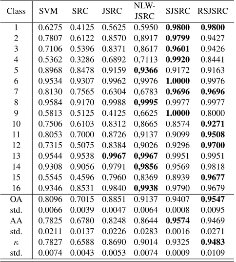
The optimal parameters of our method were p = 700, K0 = 50, λ = 0.003. For JSRC, the optimal widow size was7×7and sparsity level was 30. In NLW-JSRC, the pa-rameters were chosen from the recommendation of [15]. For SVM and SRC classifiers, we tuned the parameters such to produce the best classification results. The results are listed in Table 2. In most cases, our method RSJSRC yields bet-ter results than other classifiers. Based on super-pixel seg-mentation, SJSRC model had at least 2.7% improvement over other classical methods, such as JSRC and NLW-JSRC, which exploited the spatial information from square window with
Fig. 1. Washington DC Mall in band 41 (left) and Indian Pines image in band 31 (right).
[image:4.612.317.559.306.574.2]fixed shape and size. Considering the sparse prior for multi-ple noise in the HSIs, our proposed RSJSRC improves OA by 1.5% over SJSRC.
Table 2. Results for the Indian Pines with different classifiers.
Class SVM SRC JSRC
NLW-JSRC SJSRC RSJSRC 1 0.6275 0.4125 0.5625 0.5950 0.9800 0.9800 2 0.7807 0.6122 0.8570 0,8917 0.9799 0.9427 3 0.7106 0.5396 0.8371 0,8617 0.9601 0.9426 4 0.5362 0.3286 0.6892 0,7113 0.9920 0.8441 5 0.8968 0.8478 0.9159 0,9366 0.9172 0.9163 6 0.9534 0.9307 0.9962 0,9976 1.0000 0.9976 7 0.8130 0.7565 0.6304 0,6783 0.9696 0.9696 8 0.9584 0.9170 0.9988 0,9995 0.9977 0.9977 9 0.5813 0.5125 0.4125 0,6625 1.0000 0.8000 10 0.7506 0.6103 0.8312 0,8665 0.8574 0.9271 11 0.8053 0.7000 0.8726 0,9137 0.9099 0.9508 12 0.7315 0.5075 0.8384 0,9026 0.9296 0.9700 13 0.9544 0.9538 0.9967 0,9967 0.9951 0.9951 14 0.9308 0.9056 0.9791 0,9856 0.9569 0.9818 15 0.5545 0.4596 0.7960 0,8369 0.8939 0.9677 16 0.9346 0.8531 0.9840 0,9938 0.9790 0.9679 OA 0.8096 0.7015 0.8851 0.9137 0.9407 0.9547 std. 0.0066 0.0039 0.0047 0.0064 0.0008 0.0095 AA 0.7825 0.6780 0.8248 0.8644 0.9574 0.9469 std. 0.0211 0.0137 0.0226 0.0283 0.0016 0.0271
κ 0.7827 0.6588 0.8690 0.9014 0.9325 0.9483 std. 0.0074 0.0043 0.0053 0.0074 0.0009 0.0109
5. CONCLUSION
[image:4.612.55.294.579.688.2]6. REFERENCES
[1] B. Datt, T. R. McVicar, T. G. Van Niel, D. L. Jupp, and J. S. Pearlman, “Preprocessing eo-1 hyperion hyperspectral data to support the application of agricultural indexes,” IEEE Trans. Geosci. Remote Sens., vol. 41, no. 6, pp. 1246–1259, 2003. [2] M. T. Eismann, A. D. Stocker, and N. M. Nasrabadi,
“Au-tomated hyperspectral cueing for civilian search and rescue,”
Proceedings of the IEEE, vol. 97, no. 6, pp. 1031–1055, 2009. [3] G. Camps-Valls, D. Tuia, L. Bruzzone, and J. A. Benediktsson, “Advances in hyperspectral image classification: Earth moni-toring with statistical learning methods,”IEEE Signal Process. Mag., vol. 31, no. 1, pp. 45–54, 2014.
[4] F. Ratle, G. Camps-Valls, and J. Weston, “Semisupervised neu-ral networks for efficient hyperspectneu-ral image classification,”
IEEE Trans. Geosci. Remote Sens., vol. 48, no. 5, pp. 2271– 2282, 2010.
[5] J. Li, J. M. Bioucas-Dias, and A. Plaza, “Semisupervised hy-perspectral image segmentation using multinomial logistic re-gression with active learning,” IEEE Trans. Geosci. Remote Sens., vol. 48, no. 11, pp. 4085–4098, 2010.
[6] R. Roscher, B. Waske, and W. Forstner, “Incremental im-port vector machines for classifying hyperspectral data,”IEEE Trans. Geosci. Remote Sens., vol. 50, no. 9, pp. 3463–3473, 2012.
[7] F. Melgani and L. Bruzzone, “Classification of hyperspectral remote sensing images with support vector machines,” IEEE Trans. Geosci. Remote Sens., vol. 42, no. 8, pp. 1778–1790, 2004.
[8] D. Tuia, F. Ratle, A. Pozdnoukhov, and G. Camps-Valls, “Multisource composite kernels for urban-image classifica-tion,”IEEE Geosci. Remote Sens. Lett., vol. 7, no. 1, pp. 88–92, 2010.
[9] J. A. Benediktsson, J. A. Palmason, and J. R. Sveinsson, “Clas-sification of hyperspectral data from urban areas based on ex-tended morphological profiles,” IEEE Trans. Geosci. Remote Sens., vol. 43, no. 3, pp. 480–491, 2005.
[10] W. Liao, R. Bellens, A. Pizurica, W. Philips, and Y. Pi, “Clas-sification of hyperspectral data over urban areas using direc-tional morphological profiles and semi-supervised feature ex-traction,” IEEE J. Sel. Topics Appl. Earth Observ. in Remote Sens., vol. 5, no. 4, pp. 1177–1190, 2012.
[11] W. Liao, A. Pizurica, R. Bellens, S. Gautama, and W. Philips, “Generalized graph-based fusion of hyperspectral and lidar data using morphological features,” IEEE Geosci. Remote Sens. Lett., vol. 12, no. 3, pp. 552–556, 2015.
[12] W. Liao, M. Dalla Mura, J. Chanussot, R. Bellens, and W. Philips, “Morphological attribute profiles with partial re-construction,”IEEE Trans. Geosci. Remote Sens., vol. 54, no. 3, pp. 1738–1756, 2016.
[13] S. Prasad, M. Cui, W. Li, and J. E. Fowler, “Seg-mented mixture-of-gaussian classification for hyperspectral image analysis,” IEEE Geosci. Remote Sens. Lett., vol. 11, no. 1, pp. 138–142, 2014.
[14] Y. Chen, N. M. Nasrabadi, and T. D. Tran, “Hyperspectral image classification using dictionary-based sparse representa-tion,” IEEE Trans. Geosci. Remote Sens., vol. 49, no. 10, pp.
3973–3985, 2011.
[15] H. Zhang, J. Li, Y. Huang, and L. Zhang, “A nonlocal weighted joint sparse representation classification method for hyperspec-tral imagery,” IEEE J. Sel. Topics Appl. Earth Observ. in Re-mote Sens., vol. 7, no. 6, pp. 2056–2065, 2014.
[16] L. Fang, S. Li, X. Kang, and J. A. Benediktsson, “Spectral– spatial classification of hyperspectral images with a superpixel-based discriminative sparse model,” IEEE Trans. Geosci. Re-mote Sens., vol. 53, no. 8, pp. 4186–4201, 2015.
[17] J. Li, H. Zhang, and L. Zhang, “Efficient superpixel-level mul-titask joint sparse representation for hyperspectral image clas-sification,”IEEE Trans. Geosci. Remote Sens., vol. 53, no. 10, pp. 5338–5351, 2015.
[18] R. Roscher and B. Waske, “Shapelet-based sparse represen-tation for landcover classification of hyperspectral images,”
IEEE Trans. Geosci. Remote Sens., vol. 54, no. 3, pp. 1623– 1634, 2016.
[19] L. Fang, S. Li, X. Kang, and J. A. Benediktsson, “Spectral– spatial hyperspectral image classification via multiscale adap-tive sparse representation,”IEEE Trans. Geosci. Remote Sens., vol. 52, no. 12, pp. 7738–7749, 2014.
[20] W. Fu, S. Li, L. Fang, X. Kang, and J. A. Benediktsson, “Hy-perspectral image classification via shape-adaptive joint sparse representation,” IEEE J. Sel. Topics Appl. Earth Observ. in Remote Sens., vol. 9, no. 2, pp. 556–567, 2016.
[21] H. Zhang, W. He, L. Zhang, H. Shen, and Q. Yuan, “Hy-perspectral image restoration using low-rank matrix recovery,”
IEEE Trans. Geosci. Remote Sens., vol. 52, no. 8, pp. 4729– 4743, 2014.
[22] W. He, H. Zhang, and L. Zhang, “Sparsity-regularized robust non-negative matrix factorization for hyperspectral unmixing,”
IEEE J. Sel. Topics Appl. Earth Observ. in Remote Sens., vol. 9, no. 9, pp. 4267–4279, 2016.
[23] J. A. Tropp and A. C. Gilbert, “Signal recovery from random measurements via orthogonal matching pursuit,” IEEE Trans. Inf. Theory, vol. 53, no. 12, pp. 4655–4666, 2007.
[24] J. Wright, A. Y. Yang, A. Ganesh, S. S. Sastry, and Y. Ma, “Ro-bust face recognition via sparse representation,” IEEE Trans. Pattern Anal. Mach. Intell., vol. 31, no. 2, pp. 210–227, 2009. [25] J. A. Tropp, A. C. Gilbert, and M. J. Strauss, “Algorithms
for simultaneous sparse approximation. part i: Greedy pursuit,”
Signal Processing, vol. 86, no. 3, pp. 572–588, 2006.
[26] M. Liu, O. Tuzel, S. Ramalingam, and R. Chellappa, “En-tropy rate superpixel segmentation,” inIEEE conference on Computer Vision and Pattern Recognition (CVPR), 2011, pp. 2097–2104.
[27] D. Pham and S. Venkatesh, “Joint learning and dictionary con-struction for pattern recognition,” inIEEE conference on Com-puter Vision and Pattern Recognition (CVPR), 2008, pp. 1–8. [28] L. Bruzzone, M. Chi, and M. Marconcini, “A novel