Logistic Regression for Circular Data
Kadhem Al-Da
ff
aie
1,2,a)and Shahjahan Khan
3,b)1School of Agricultural, Computational and Environmental Sciences
University of Southern Queensland, Toowoomba, QLD, Australia
2Al-Muthana University, Al-Muthana, Iraq
3School of Agricultural, Computational and Environmental Sciences
International Centre for Applied Climate Research Science University of Southern Queensland, Toowoomba, QLD, Australia
a)Kadhem.Aldaff[email protected] b)[email protected]
Abstract.This paper considers the relationship between a binary response and a circular predictor. It develops the logistic regression model by employing the linear-circular regression approach. The maximum likelihood method is used to estimate the parameters. The Newton-Raphson numerical method is used to find the estimated values of the parameters. A data set from weather records of Toowoomba city is analysed by the proposed methods. Moreover, a simulation study is considered. The R software is used for all computations and simulations.
INTRODUCTION
There are two types of data, namely linear and circular data. The most common type is linear data such as observations on income, age, weight, numbers of any item and so on. Whereas, according to [1] the second type occurs when directions are measured. He states that time data, for example, measured on a 24 hour clock may be considered as circular data by converting them to angular data. Therefore, data measured by compass or clock, can be expressed in degrees from 00 to 3600 or in radians from 0 to 2π(cf. [2], [3] and [4]). Circular data can be found in many different fields, for instance in meteorology, physics, psychology, medicine and biology. The wind direction or the flight directions of bird-migrations are some examples of this type of data.
Statistical methods developed for linear data normally do not work for circular data. However, many statistical tools have been proposed to treat this type of data. These tools are called circular or directional statistics. They differ from those which are used for the linear data. These differences are formed in many aspects of statistical analysis, such as data display, descriptive and inferential statistics, mathematical distributions, regression analysis and beyond [5, Chapter 1]. Despite the nature of each type of the data, almost all statistical topics can be considered for both linear and circular data. One of the useful statistical tools is logistic regression analysis, which analyses the relationship between a binary response and a predictor. This paper deals with the logistic regression analysis for circular data.
Descriptive statistics for circular data
The early appearance of observations of a circular nature occurred in geology. [6, pp.11-13] summarises the first use of descriptive statistics for circular data, reporting that the key idea of transforming the circular data to vectors was introduced by Krumbein in 1939, which is essential in the analysing process of this type of observations. [6, pp.11-13] also reports that researchers later developed some measures for circular data such as the mean direction and circular variance. Fisher [6, pp. 30-35], [5, pp.9-15], [1] and [4, pp.13-19] also introduce some processes of finding descriptive statistics.
to the starting point and a sense of rotation. They also can be represented as points on the circumference of a unit circle or as unit vectors from the origin as only the direction is required. Due to this circular representation, such observations are called circular data. We can specify any point on a plane by an ordered pair of numbers, called the coordinates of the point. Two coordinate systems are used for this purpose:
1. the rectangular coordinate system, representing a point on a plane as (x,y);
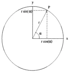
[image:2.612.248.368.174.300.2]2. the polar coordinate system, using (r, α) to represent any point, whereris the distance to the origin andαis the angle as shown in Figure 1 bellow.
FIGURE 1.Relation between rectangular and polar co-ordinates.
Note that, it is easy to convert between these two systems by using trigonometry. As in figure 1, the relationship between rectangular coordinates and polar coordinates is
x=rcosα,y=rsinα. (1)
Since the interest is only in the direction of the points and not in their magnitude,ris always considered 1. Thus, there is a point on the circumference of the unit circle that corresponds to each direction. Each point is then described by the angle only. Therefore the equation (1) simply becomes
x=cosα,y=sinα. (2)
Now as the circular data have a special nature, special techniques are needed to measure their descriptive statistics. Thus instead of using the arithmetic mean to measure the mean direction for a set of directions, another measurement called the circular mean direction is used instead. It is calculated by treating the data as unit vectors and finding the direction of their resultant vector.
For example suppose there is a set of circular data given in terms of anglesα1, α2,· · ·, αn wherenis the number of
observations. Using equation (2), the transformation from polar to rectangular coordinates leads to the observations
(cosαi, sinαi), i=1,· · ·n. (3)
The resultant vectorRthen becomes
R=
Xn
i=1
cosαi, n
X
i=1
sinαi
=(C,S),say. (4)
The direction of this resultant vector is the circular mean direction. The notation ¯α0is used to denote the circular mean
direction which is given by
¯
α0=arctan(S/C). (5)
Moreover, as an alternative measure of variance, the length of the resultant vector is used as a measure of concentration of a data set. Which defined as
R=kRk= √
Regression model
To present the relationship between two or more quantitative variables, statisticians use regression models. Depend-ing on the nature of these variables, these models are divided into two types: linear regression models and circular regression models.
Linear regression model
Linear regression models are used to describe the relationship between two or more quantitative variables that are linear in nature. One of these variables is called a dependent variable and the rest are called independent variables. For the simplest case, when there are only two linear variables, the model takes the form:
Yi=β0+β1Xi+i, i=1,· · ·,n, (7) whereYi is theith value of the dependent variable,β0 andβ1 are regression parameters, Xi is theithvalue of the
independent variable andiis a random error term. For more details, see [7, p.31], [8, p.3], [9, p.75], [10, p.13] and [11, pp.8-9].
Circular - linear regression model
The circular-linear regression model is used to represent the relationship between a linear response variable and one or more circular predictor variables. [12] proposes a method to determine the correlation coefficient between a linear variable and a circular variable. It introduces the regression formulaz=a+bcosθ+csinθ, wherezis a linear variable andθis a circular variable. This particular form of the model makes the coefficient of the multiple correlation of x with (cosθ,sinθ) equal to one.
Later [13] suggests a regression model to represent the relationship between a linear response and a circular predictor. [14] proposes a correlation coefficient between two variables which are of different types, i.e linear, circular or di-rectional. They also give a circular-linear regression model, which is exactly the same as that proposed by [13]. The estimates of the parameters are also the same despite using the least square estimating method. The same model also appears in [6, p.139], [4, p.257] and [5, p.186].
The article [15] introduces a regression model to represent the relationship between a linear response with a circular predictor and a set of linear covariates. [16] provides a case study to illustrate the importance of circular statistics in analysing the relationship between the ozone level and the wind direction.
The book [17] also contains this model with relevant explanations on how to analyse some circular data sets using the R-program.
In short, suppose there is a sample (y1, θ1), . . . ,(yn, θn), whereyiis a linear response andθiis a circular predictor. The
model is given by
Y =β0+Acos(θi−θ0), (8)
whereβ0represents the mean value of the response when (θi−θ0 =90),Ais the amplitude of the cyclic fluctuation
in the response, andθ0 is the highest point that the curve “response value” can reach also known as the “acrophase
angle” (cf. [5, p.186]).
Logistic regression model
Logistic regression analysis is a statistical tool employed to study the relationship between a categorical response and predictors. This model may be divided into two types depending on the nature of the predictors, whether they are linear or circular.
Logistic regression model for linear data
and with the improvement of the statistical software, the maximum likelihood method was used with some numerical methods to estimate the model parameters. The logistic regression model is used to analyse the relation between some predictors and a binary response. It models the probability that the response belongs to a particular category, such as 0 or 1; success or failure, rather than modeling the response directly. To explain this model, consider the following logical steps.
1. Assume there is a binary responser, wherer=0 or 1.
2. Assume there arenof these binary responses, the jth one denoted byrj; where j=1,2,· · ·,nand eachrjis either 0 or 1.
3. Assume the number of successes “i.e whenrjtakes the value 1” in thesenobservations is denoted byy, where y=r1+r2+· · ·+rn(≤n).
4. Now assume thesenobservations are divided intokgroups, each one withniobservations, wherei=1,2,· · ·,k andPk
i=1ni =n. As a result, for theith group the number of successes is denoted byyi. These observations are
from a binomial distribution.
5. Next define yi
ni which is a proportion of “successes” denoted by pi. These proportions represent the success probability.
6. Finally, model the dependence of this success probabilitypion some explanatory variables. A linear regression model is used to build such a model. However, the use of a model such as
pi=β0+β1x1+· · ·+βkxk, (9)
is misleading. In other word, the term on the left hand side has a range (0,1); whereas, the term on the right hand side can assume any value on the real line. For this reason, the probability scale has to be changed from the range (0,1) to the range (−∞,∞). According to [20, p.56] one of the possible transformations that can be applied is the logit of a success probabilityp, which is written as
logitp=log p
1−p. (10)
Note that the 1−pp is the odds of a success, given by the ratio of the probability of success over the probability of failure. So the logit transformation of pis the logarithm of odds of a success. The range of the logit value for any value ofpis (−∞,∞). This step enables us to model the dependence of the success probability on some explanatory variables by using linear logistic regression as
logit(pi)=log
p
i 1−pi
=β0+β1x1+· · ·+βkxk, (11)
which after some simplifications may be written as
pi= e
β0Pki=1βixi
1+β0Pki=1βixi
. (12)
The latter equation shows how the logistic regression model is used to model the probability of a response belonging to a particular category depending on some predictors.
For more details see [20, Sections 2.1, 3.5 & 3.6] and [21, Section 1.1].
Logistic regression model for circular data
Modelling
For the circular logistic regression model, this paper will cover the case of only one circular variable as a predictor. Considernbinomial observations withpi= yi
ni, fori=1, . . . ,k. Let the value ofpidepends on a circular variableθias follows:
logit(pi)=log pi 1−pi
=β0+Acos(θi−θ0), (13)
where
• β0is the value of the logit (log odds) when the result angle from the term (θi−θ0) equals 900, or equivalently
eβ0is the value the odds when the result angle from the term (θ
i−θ0) equals 900.
• Arepresents the distance from thexaxis to the highest point in the curve or it is the amplitude of the cyclic fluctuation in the response.
• θ0is the angle where the logit (log odds) reaches its highest value.
Equation (13) can be written as
logit(pi)=log
pi 1−pi
=β0+β1cosθi+β2sinθi, (14)
where
A=
q
β2 1+β
2
2andθ0=tan
−1(β
2/β1). (15)
Now to simplify the estimating process, equation (14) may be rewritten by assumingηi=β0+β1cosθi+β2sinθiand
using the exponential function to obtain
pi 1−pi =e
ηi ⇒p i=
eηi
(1+eηi) (16)
Estimation of parameters
The maximum likelihood method will be used to estimate the parameters,β0, β1andβ2, of the circular logistic
regres-sion model. Suppose that binomial data of the formyisuccesses out ofnitrials,i=1,· · ·,k, are observations from a binomial distribution. The likelihood function is then given by
L(β)= n
Y
i=1
ni yi
!
pyi
i(1−pi)ni−yi. (17)
This likelihood function depends on the unknownpiwhich depends on the regression coefficientsβ0sthrough equation
(14).
We need to find the estimators ˆβ0,βˆ1and ˆβ2which maximises the functionL(β)
logL(β)= k
X
i=1
(
log ni yi
!
+yilogpi+(ni−yi) log(1−pi)
)
. (18)
After some algebraic operations and using some derivation rules, the first derivatives of the parametersβ0, β1andβ2
can be written as follows
∂logL(β) ∂β0 =
k
X
i=1
yi−
k
X
i=1
ni
1+e−(β0+β1cosθ+β2sinθ), (19)
∂logL(β) ∂β1 =
k
X
i=1
yicosθ−
k
X
i=1
nicosθ
1+e−(β0+β1cosθ+β2sinθ), (20)
∂logL(β) ∂β2 =
k
X
i=1
yisinθ−
k
X
i=1
nisinθ 1+e−(β0+β1cosθ+β2sinθ)
Due to the complicated nature of this function, the derivatives are unavailable in any explicit form. As an alternative, the Newton-Raphson method is used to estimate the parameters of the model [22, Section 12.3.2] with an initial value ofβ(t)in the following formula
β(t+1)=β(t)+h
−l00(β(t))i−1l0(β(t)), (22) and then repeat this step until gettingβ(t+1) ≈β(t).Once we obtain the estimated values ofβ0, β1 andβ2, we should
apply the equations (15) to get fitted the circular logistic regression model.
Goodness of fit test
The goodness of fit test used to determine how well a model fits a set of data. It compares the observed values with the predicted values. One of the measures used to do this test is the deviance. [21, p.12] and [20, Section 3.8] mention how to use the deviance to test the goodness of fit for the linear logistic regression. The same process will be adopted to handle the goodness of fit test for the circular logistic regression model. For binomial data, the deviance measures the difference between the observed binomial proportions, yi
ni denoted by pi, and the predicted proportions, ˆpi, under an assumed model for the true success probabilitypi. The likelihood function of the predicted model, which contains the predicted value ˆpi, denoted byLp, will be compared to that of the observed model, which contains the observed valuepi= yi
ni and will be denoted byLo. The comparison is achieved by using the deviance statistic which is given by the formula
D=−2 log(Lp/Lo)=−2(logLp−logLo)· (23) For the circular logistic regression, the predicted values ˆpiare obtained by
logit(ˆpi)=βˆ0+βˆ1cosθi+βˆ2cosθi. (24)
From the equation (18), the maximised log-likelihood function under the predicted function is
logLp= k
X
i=1
(
log ni yi
!
+yilog ˆpi+(ni−yi) log(1−piˆ)
)
. (25)
While under the observed model, the fitted probabilities will be the same as the observed proportions, pi = yi/ni, i=1,2, ...,k, and so the maximised log-likelihood function for the observed model is
logLo= k
X
i=1
(
log ni yi
!
+yilogpi+(ni−yi) log(1−pi)
)
. (26)
The deviance is then given by
D = −2(logLp−logLo)
= −2
k
X
i=1
(
yilogpi ˆ pi
+(ni−yi) log
1−pi
1−pˆi
)
. (27)
The predicted number of successes is ˆyi=nipiˆ, then the latter equation can be written as
D=−2 k
X
i=1
(
yilogyi ˆ yi
+(ni−yi) log
ni−yi
ni−yˆi
)
. (28)
It is easily seen that this is a statistic compares the observationsyiwith their corresponding fitted values ˆyiunder the current model. The deviance is asymptotically distributed as the chi-square distribution,χ2, with (k−p) degrees of
freedom, wherekis the number of binomial observations (i.e the actual number of proportionsyi
ni), andpis the number of unknown parameters in the current linear logistic model. According to [23], the goodness of fit tests the following hypotheses:
H0: model does not fit vs.H1 : model fits. (29)
Application of Circular Logistic Regression model
In this part, a real data set is analysed to demonstrate the proposed method. This data set was obtained from the Aus-tralian Bureau of Meteorology for the Toowoomba Airport weather station which is located in Toowoomba, Queens-land, Australia. It contains 365 daily observations of rainfall records (yes or no) and wind directions measured in degrees from January 1 to December 31 in 2015. To verify the proposed approach, a simulation study is conducted, which gives acceptable results. The R software [24] is used to conduct the simulation and the analysis of the real data.
Illustration with Simulation
To simulate data for fitting a circular logistic regression model, the following two R-packages are used
1. CircStatsis used to generate circular variables [25]. According to [5, p.54] the function “rvm” is used to gen-erate a set of circular random variables from the von Mises distributionCN(µ, κ). This function has 3 arguments namely sample size, mean directionµand concentration parameterκ
2. ISwRis used to run the proposed model [26]. The function “glm” is used to fit a linear logistic regression model [27, p.228]. This function is adopted to fit a circular logistic regression model.
Firstly, a circular predictor vector “cir.pred.” is generated fromCN(600,12) withn =1000. After that calculate the
probability of success using equation (16) and by settingβ0=1, β1=2 andβ2=3. Furthermore, a binary response is
generated using the above results and the function “rbinom”. The generated data are saved in a file called Sim.Data. Finally, the proposed model is fitted by using the adapted version of the function “glm” as shown bellow.
glm(formula = Bin.resp. ~ cos(cir.pred.) + sin(cir.pred.), family = "binomial",data =Sim.Data) Deviance Residuals:
Min 1Q Median 3Q Max
-2.9583 -0.4631 0.1661 0.4247 2.2974
Coefficients:
Estimate Std. Error z value Pr(>|z|)
(Intercept) 0.9091 0.1102 8.248 <2e-16 ***
cos(cir.pred.) 1.7947 0.1449 12.387 <2e-16 ***
sin(cir.pred.) 3.0327 0.1840 16.478 <2e-16 ***
---Signif. codes: 0 *** 0.001 ** 0.01 * 0.05 . 0.1 1
(Dispersion parameter for binomial family taken to be 1)
Null deviance: 1351.50 on 999 degrees of freedom
Residual deviance: 688.63 on 997 degrees of freedom
AIC: 694.63
Number of Fisher Scoring iterations: 5 The p-value is 1.151929e-144
These results show that the proposed model as a whole fits much better than the null model. In addition, this model does very well when it comes to calculate the associated probabilities with each predictor. It shows that these values vary from 0 to 1. Furthermore, it could be used to predict the probability of the success of the response for any pre-selected value of the circular predictor.
Analysis of Rainfall Data
glm(formula = R ~ cos(W) + sin(W), family = binomial(link = "logit"), data = Rain.Wind)
Deviance Residuals:
Min 1Q Median 3Q Max
-1.0534 -0.9080 -0.7408 1.3383 1.7238
Coefficients:
Estimate Std. Error z value Pr(>|z|)
(Intercept) -0.76292 0.11404 -6.690 2.23e-11 ***
cos(W) -0.04106 0.16237 -0.253 0.80037
sin(W) 0.46436 0.16050 2.893 0.00381 **
---Signif. codes: 0 *** 0.001 ** 0.01 * 0.05 . 0.1 1
(Dispersion parameter for binomial family taken to be 1)
Null deviance: 454.86 on 364 degrees of freedom
Residual deviance: 446.33 on 362 degrees of freedom
AIC: 452.33
Number of Fisher Scoring iterations: 4 The p-value is 0.01404355
The predicted value of the associated probability with W=78 is 0.3801237
As shown in equation (29) above, a chi-square value of 8.53 on 2 degrees of freedom yields a p-value of 0.014. That means the the null hypothesis, which says model does not fit, is rejected.
Now, the estimated values of the parameters are used to fit the proposed model. By using equation (15), the estimated value of the parameters of the proposed model are A ' 0.46 and θ0 = 95.050. As a result, the circular logistic
regression model of the relation between the rainfall as a response and the wind direction as a circular predictor of the considered data set is given by
logit(pi)=log( pi
1−pi)=−0.762+0.46 cos (θi−95.05
0)
where
• β0=0.762 is the value of the logit (pi) or log (odds) when the resulted angle from the term (θi−95.050) equals
900, or equivalentlyeβ0is the value the odds when the resulted angle from the term (θ
i−95.050) equals 900.
• A=0.46 represents the distance from the horizontal axis to the highest point in the curve or it is the amplitude of the cyclic fluctuation in the response.
• θ0=95.050is the angle where the logit (pi) or log (odds) reaches its highest value.
Conclusion
This paper has provided a new logistic regression model to analyse the relationship between a binary response and a circular predictor. This model is capable of calculating the associated probability with each value of the circular predictor variable and to predict the success probability of the response at any chosen value of the circular predictor variable.
ACKNOWLEDGMENTS
REFERENCES
[1] A. Lee, Wiley Interdisciplinary Reviews: Computational Statistics2, 477–486 (2010).
[2] A. Scott,Circular Data: An Overview with Discussion of One-Sample Tests, Master’s thesis, Montana State University (2002).
[3] V. Deva Raaj, “Some contributions to circular statistics,” Unpublished phd thesis, Acharya Nagarjuna Uni-versity 2013.
[4] K. V. Mardia and P. E. Jupp,Directional statistics, Wiley Series in Probability and Statistics (John Wiley & Sons, Ltd, Chichester, 2000).
[5] S. R. Jammalamadaka and A. Sengupta,Topics in circular statistics, Series on multivariate analysis, Vol. 5 (World Scientific, Singapore, 2001).
[6] N. I. Fisher,Statistical analysis of circular data(Cambridge University Press, Cambridge, 1993).
[7] J. Neter, W. Wasserman, and M. H. Kutner,Applied linear statistical models: regression, analysis of vari-ance, and experimental designs, 3rd ed. (Richard D. Irwin, Inc., Boston, 1990).
[8] T. P. Ryan,Modern regression methods, Wiley Series in Probability and Statistics (John Wiley & Sons, Inc., New York, 1997).
[9] J. H. Stapleton,Linear statistical models, The Wiley Series in Probability and Statistics (John Wiley & Sons, Inc., New York, 1995).
[10] D. C. Montgomery, E. A. Peck, and G. G. Vining,Introduction to linear regression analysis, 3rd ed., Wiley Series in Probability and Statistics (John Wiley & Sons, Inc., New York, 2001).
[11] R. H. Myers,Classical and modern regression with applications, 2nd ed. (PWS-KENT Publishing Company, California, 1990).
[12] K. V. Mardia, Biometrika63, 403–405 (1976).
[13] K. Mardia and T. Sutton, Journal of the Royal Statistical Society. Series B (Methodological)40, 229–233 (1978).
[14] P. Jupp and K. Mardia, Biometrika67, 163–173 (1980).
[15] A. SenGupta and F. I. Ugwuowo, Environmental and Ecological Statistics13, 299–309 (2006). [16] S. R. Jammalamadaka and U. J. Lund, Environmental and Ecological Statistics13, 287–298 (2006). [17] A. Pewsey, M. Neuh¨auser, and G. Ruxton,Circular Statistics in R, EBL-Schweitzer (OUP, Oxford, 2013). [18] J. Cramer,Logit Models from Economics and Other Fields(Cambridge University Press, Cambridge, 2003). [19] J. M. Hilbe,Logistic regression models(Taylor & Francis Group , LLC, Florida, 2009).
[20] D. Collett,Modelling binary data, 2nd ed. (Chapman & Hall/CRC, Florida, 2003).
[21] D. W. Hosmer and S. Lemeshow,Applied logistic regression(John Wiley & Sons, Inc., New York, 1989). [22] S. Weisberg,Applied linear regression, 3rd ed., Wiley Series in Probability and Statistics (John Wiley &
Sons, Inc., New Jersey, 2005).
[23] D. Kleinbaum and M. Klein,Logistic Regression: A Self-Learning Text, 3rd ed., Statistics for Biology and Health (Springer, New York, 2010).
[24] R Core Team,R: A Language and Environment for Statistical Computing, R Foundation for Statistical Com-puting, Vienna, Austria (2013).
[25] S. plus original by Ulric Lund and R. port by Claudio Agostinelli,CircStats: Circular Statistics, from ”Topics in circular Statistics” (2001)(2012), r package version 0.2-4.